
A New Anisotropic Four-Parameter Turbulence Model for Low Prandtl Number Fluids


Abstract
:1. Introduction
2. Mathematical Model
2.1. Dynamic Turbulence Modeling
2.2. Thermal Turbulence Modeling
2.3. Boundary Conditions
3. Numerical Results and Validation of the A4P Model
3.1. Plane Channel Geometry
3.2. Backward Facing Step Geometry
3.3. Dynamical Fields
3.4. Thermal Fields
4. Conclusions
Author Contributions
Funding
Institutional Review Board Statement
Informed Consent Statement
Data Availability Statement
Conflicts of Interest
References
- Heinzel, A.; Hering, W.; Konys, J.; Marocco, L.; Litfin, K.; Müller, G.; Pacio, J.; Schroer, C.; Stieglitz, R.; Stoppel, L.; et al. Liquid Metals as Efficient High-Temperature Heat-Transport Fluids. Energy Technol. 2017, 5, 1026–1036. [Google Scholar] [CrossRef] [Green Version]
- Marocco, L.; Cammi, G.; Flesch, J.; Wetzel, T. Numerical analysis of a solar tower receiver tube operated with liquid metals. Int. J. Therm. Sci. 2016, 105, 22–35. [Google Scholar] [CrossRef]
- Frazer, D.; Stergar, E.; Cionea, C.; Hosemann, P. Liquid metal as a heat transport fluid for thermal solar power applications. Energy Procedia 2014, 49, 627–636. [Google Scholar] [CrossRef] [Green Version]
- Manservisi, S.; Menghini, F. Triangular rod bundle simulations of a CFD κ-ε-κθ-εθ heat transfer turbulence model for heavy liquid metals. Nucl. Eng. Des. 2014, 273, 251–270. [Google Scholar] [CrossRef]
- Cheng, X.; Tak, N. Investigation on turbulent heat transfer to lead–bismuth eutectic flows in circular tubes for nuclear applications. Nucl. Eng. Des. 2006, 236, 385–393. [Google Scholar] [CrossRef]
- Pacio, J.; Litfin, K.; Batta, A.; Viellieber, M.; Class, A.; Doolaard, H.; Roelofs, F.; Manservisi, S.; Menghini, F.; Böttcher, M. Heat transfer to liquid metals in a hexagonal rod bundle with grid spacers: Experimental and simulation results. Nucl. Eng. Des. 2015, 290, 27–39. [Google Scholar] [CrossRef]
- Schulenberg, T.; Stieglitz, R. Flow measurement techniques in heavy liquid metals. Nucl. Eng. Des. 2010, 240, 2077–2087. [Google Scholar] [CrossRef]
- Grötzbach, G. Challenges in low-Prandtl number heat transfer simulation and modelling. Nucl. Eng. Des. 2013, 264, 41–55. [Google Scholar] [CrossRef]
- Grötzbach, G. Anisotropy and Buoyancy in Nuclear Turbulent Heat Transfer: Critical Assessment and Needs for Modelling; Citeseer: University Park, PA, USA, 2007. [Google Scholar]
- Shams, A.; De Santis, A.; Koloszar, L.; Ortiz, A.V.; Narayanan, C. Status and perspectives of turbulent heat transfer modelling in low-Prandtl number fluids. Nucl. Eng. Des. 2019, 353, 110220. [Google Scholar] [CrossRef]
- De Santis, A.; Shams, A. Application of an algebraic turbulent heat flux model to a backward facing step flow at low Prandtl number. Ann. Nucl. Energy 2018, 117, 32–44. [Google Scholar] [CrossRef]
- Shams, A.; De Santis, A. Towards the accurate prediction of the turbulent flow and heat transfer in low-Prandtl fluids. Int. J. Heat Mass Transf. 2019, 130, 290–303. [Google Scholar] [CrossRef]
- Manservisi, S.; Menghini, F. A CFD four parameter heat transfer turbulence model for engineering applications in heavy liquid metals. Int. J. Heat Mass Transf. 2014, 69, 312–326. [Google Scholar] [CrossRef]
- Da Via, R.; Manservisi, S.; Menghini, F. A k-Ω-kθ-Ωθ four parameter logarithmic turbulence model for liquid metals. Int. J. Heat Mass Transf. 2016, 101, 1030–1041. [Google Scholar] [CrossRef]
- Da Vià, R.; Giovacchini, V.; Manservisi, S. A Logarithmic Turbulent Heat Transfer Model in Applications with Liquid Metals for Pr = 0.01–0.025. Appl. Sci. 2020, 10, 4337. [Google Scholar] [CrossRef]
- Da Vià, R.; Manservisi, S. Numerical simulation of forced and mixed convection turbulent liquid sodium flow over a vertical backward facing step with a four parameter turbulence model. Int. J. Heat Mass Transf. 2019, 135, 591–603. [Google Scholar] [CrossRef]
- Kawamura, H.; Abe, H.; Matsuo, Y. DNS of turbulent heat transfer in channel flow with respect to Reynolds and Prandtl number effects. Int. J. Heat Fluid Flow 1999, 20, 196–207. [Google Scholar] [CrossRef]
- Abe, H.; Kawamura, H.; Matsuo, Y. Surface heat-flux fluctuations in a turbulent channel flow up to Reτ = 1020 with Pr = 0.025 and 0.71. Int. J. Heat Fluid Flow 2004, 25, 404–419. [Google Scholar] [CrossRef]
- Tiselj, I.; Cizelj, L. DNS of turbulent channel flow with conjugate heat transfer at Prandtl number 0.01. Nucl. Eng. Des. 2012, 253, 153–160. [Google Scholar] [CrossRef]
- Alcántara-Ávila, F.; Hoyas, S.; Pérez-Quiles, M.J. DNS of thermal channel flow up to Reτ = 2000 for medium to low Prandtl numbers. Int. J. Heat Mass Transf. 2018, 127, 349–361. [Google Scholar] [CrossRef]
- Niemann, M.; Fröhlich, J. Direct Numerical Simulation of turbulent heat transfer behind a backward-facing step at low Prandtl number. PAMM 2014, 14, 659–660. [Google Scholar] [CrossRef]
- Niemann, M.; Fröhlich, J. Buoyancy-affected backward-facing step flow with heat transfer at low Prandtl number. Int. J. Heat Mass Transf. 2016, 101, 1237–1250. [Google Scholar] [CrossRef]
- Abe, K.; Kondoh, T.; Nagano, Y. On Reynolds-stress expressions and near-wall scaling parameters for predicting wall and homogeneous turbulent shear flows. Int. J. Heat Fluid Flow 1997, 18, 266–282. [Google Scholar] [CrossRef]
- Hattori, H.; Morita, A.; Nagano, Y. Nonlinear eddy diffusivity models reflecting buoyancy effect for wall-shear flows and heat transfer. Int. J. Heat Fluid Flow 2006, 27, 671–683. [Google Scholar] [CrossRef]
- Abe, K.; Kondoh, T.; Nagano, Y. A new turbulence model for predicting fluid flow and heat transfer in separating and reattaching flows—I. Flow field calculations. Int. J. Heat Mass. Transf. 1994, 37, 139–151. [Google Scholar] [CrossRef]
- Ilinca, F.; Pelletier, D. A unified finite element algorithm for two-equation models of turbulence. Comput. Fluids 1998, 27, 291–310. [Google Scholar] [CrossRef]
- Abe, K.; Kondoh, T.; Nagano, Y. A two-equation heat transfer model reflecting second-moment closures for wall and free turbulent flows. Int. J. Heat Fluid Flow 1996, 17, 228–237. [Google Scholar] [CrossRef]
- Kays, W.M. Turbulent Prandtl number. Where are we? ASME Trans. J. Heat Transf. 1994, 116, 284–295. [Google Scholar] [CrossRef]
- Abe, K.; Kondoh, T.; Nagano, Y. A new turbulence model for predicting fluid flow and heat transfer in separating and reattaching flows—II. Thermal field calculations. Int. J. Heat Mass Transf. 1995, 38, 1467–1481. [Google Scholar] [CrossRef]
- Nagano, Y.; Shimada, M. Development of a two-equation heat transfer model based on direct simulations of turbulent flows with different Prandtl numbers. Phys. Fluids 1996, 8, 3379–3402. [Google Scholar] [CrossRef]
- Chierici, A.; Barbi, G.; Bornia, G.; Cerroni, D.; Chirco, L.; Da Vià, R.; Giovacchini, V.; Manservisi, S.; Scardovelli, R.; Cervone, A. FEMuS-Platform: A numerical platform for multiscale and multiphysics code coupling. In Proceedings of the 9th Edition of the International Conference on Computational Methods for Coupled Problems in Science and Engineering, Sardinia, Italy, 13–16 June 2021. [Google Scholar]
- Moin, P.; Kim, J. Numerical investigation of turbulent channel flow. J. Fluid Mech. 1982, 118, 341–377. [Google Scholar] [CrossRef] [Green Version]
- Vreman, A.; Kuerten, J.G. Comparison of direct numerical simulation databases of turbulent channel flow at Reτ = 180. Phys. Fluids 2014, 26, 015102. [Google Scholar] [CrossRef] [Green Version]
- Niemann, M.; Fröhlich, J. Buoyancy Effects on Turbulent Heat Transfer Behind a Backward-Facing Step in Liquid Metal Flow. In Direct and Large-Eddy Simulation X; Springer: Berlin/Heidelberg, Germany, 2018; pp. 513–519. [Google Scholar]
- Niemann, M.; Fröhlich, J. Turbulence budgets in buoyancy-affected vertical backward-facing step flow at low Prandtl number. Flow Turbul. Combust. 2017, 99, 705–728. [Google Scholar] [CrossRef]
- Schumm, T.; Niemann, M.; Magagnato, F.; Marocco, L.; Frohnapfel, B.; Fröhlich, J. Numerical prediction of heat transfer in liquid metal applications. In Proceedings of the Eighth International Symposium on Turbulence Heat and Mass Transfer, THMT-15, Sarajevo, Bosnia and Herzegovina, 15–18 September 2015. [Google Scholar]
- Manservisi, S.; Menghini, F. CFD simulations in heavy liquid metal flows for square lattice bare rod bundle geometries with a four parameter heat transfer turbulence model. Nucl. Eng. Des. 2015, 295, 251–260. [Google Scholar] [CrossRef]
- Kasagi, N.; Matsunaga, A. Three-dimensional particle-tracking velocimetry measurement of turbulence statistics and energy budget in a backward-facing step flow. Int. J. Heat Fluid Flow 1995, 16, 477–485. [Google Scholar] [CrossRef]


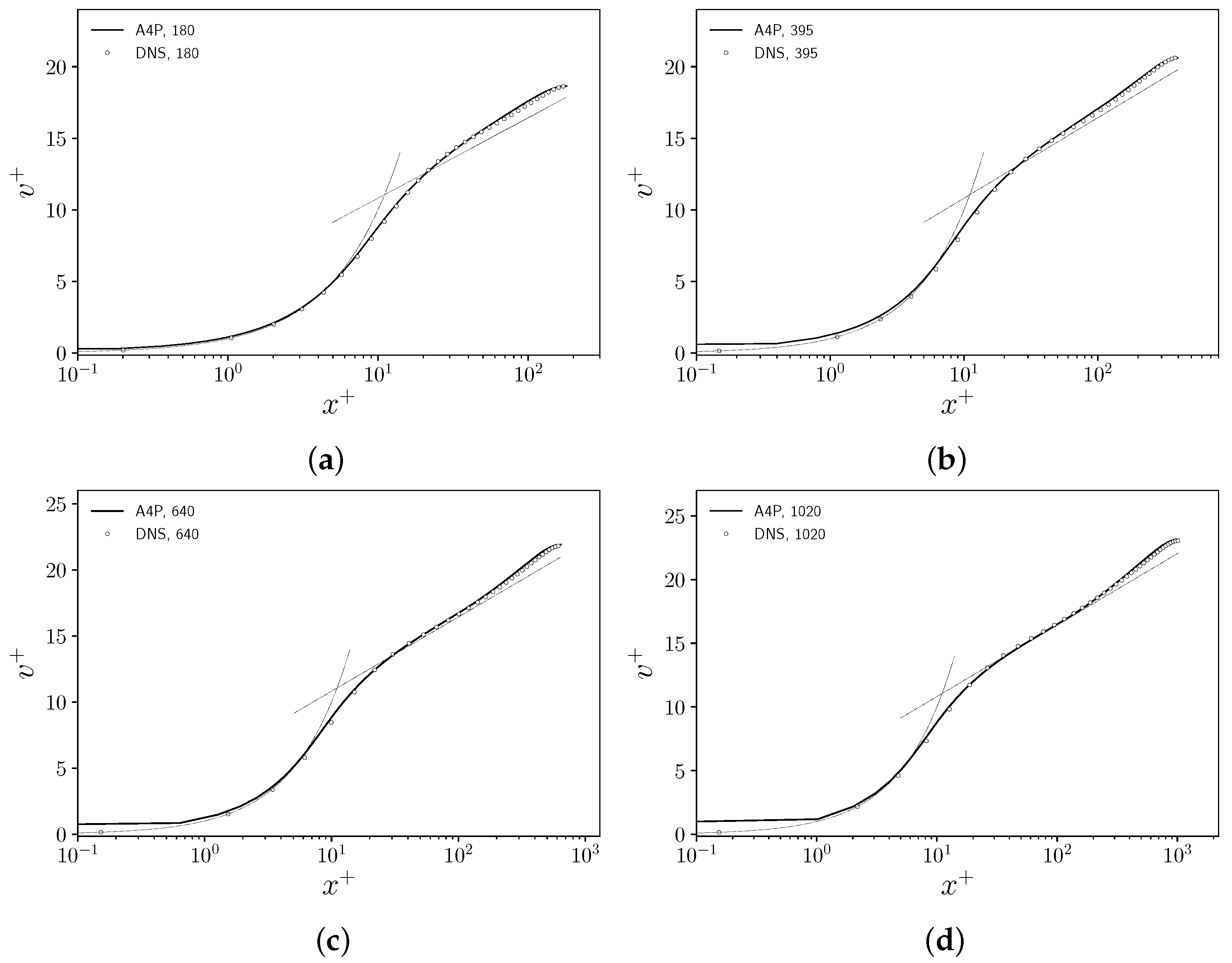
 : Simulation results with the anisotropic four-parameter (A4P) model;
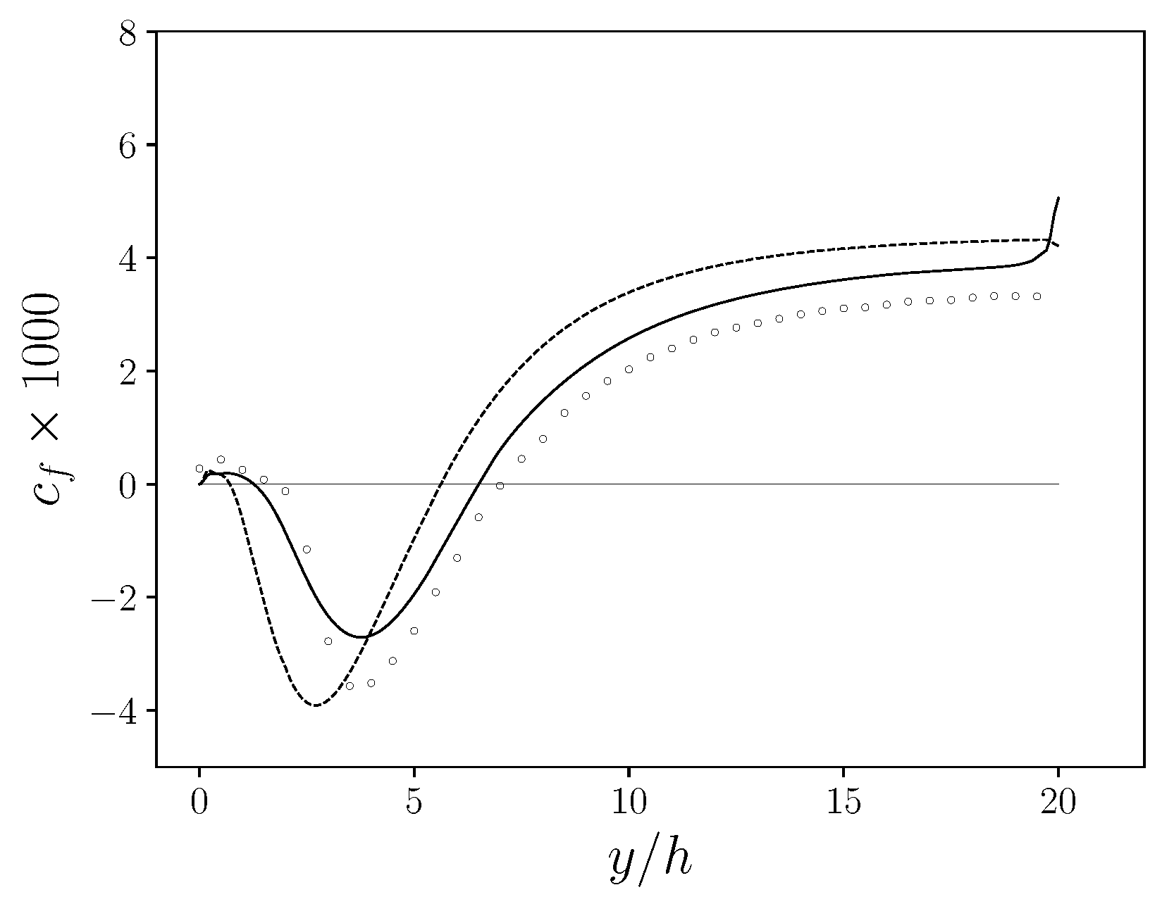
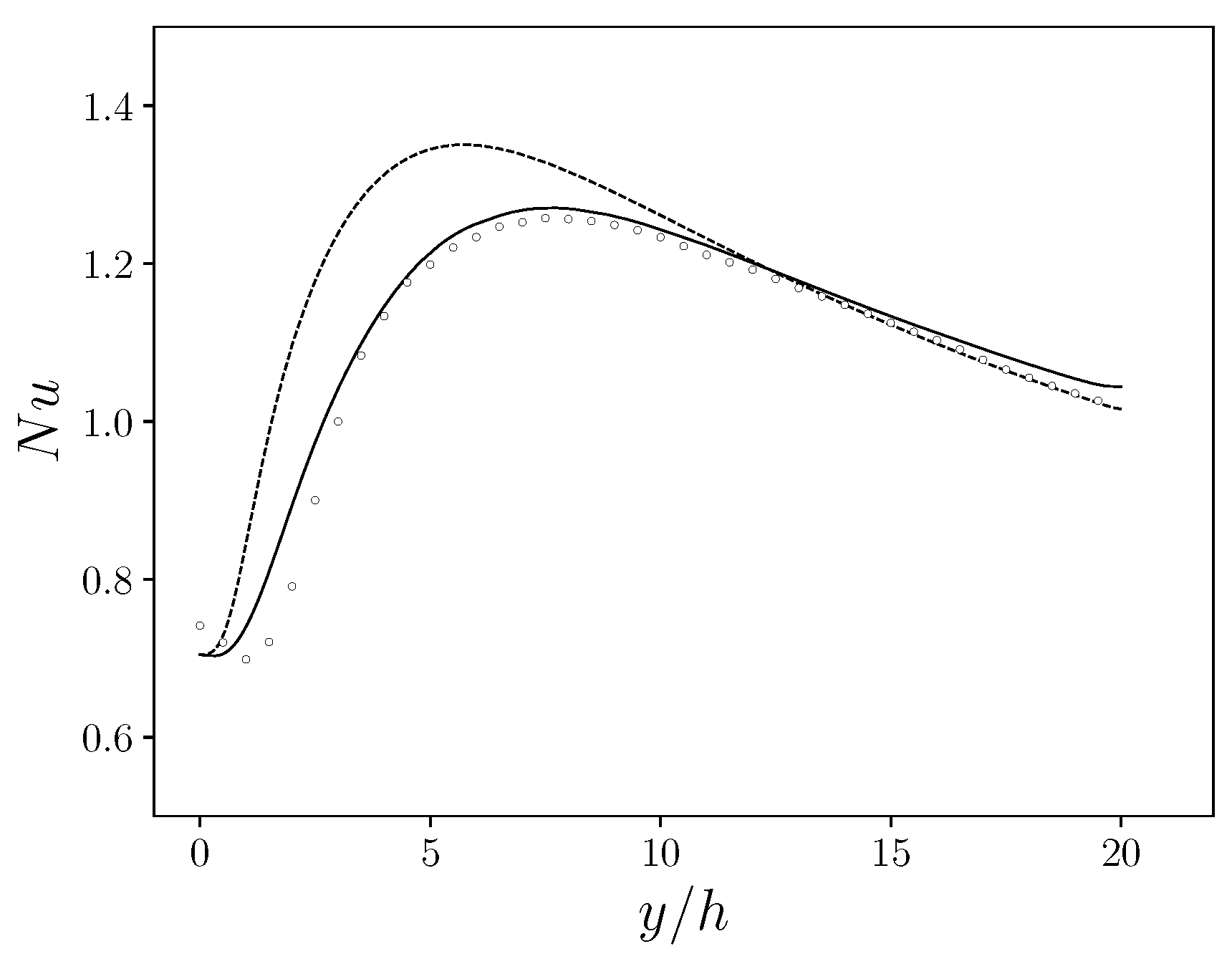
  : Simulation results with the isotropic four-parameter (4P) model. ∘: DNS data.
: Simulation results with the anisotropic four-parameter (A4P) model; : Simulation results with the isotropic four-parameter (4P) model. ∘: DNS data.
: Simulation results with the isotropic four-parameter (4P) model. ∘: DNS data.
: Simulation results with the anisotropic four-parameter (A4P) model; : Simulation results with the isotropic four-parameter (4P) model. ∘: DNS data. : Simulation results with the anisotropic four-parameter (A4P) model; : Simulation results with the isotropic four-parameter (4P) model. ∘: DNS data.
: Simulation results with the anisotropic four-parameter (A4P) model; : Simulation results with the isotropic four-parameter (4P) model. ∘: DNS data.
: Simulation results with the anisotropic four-parameter (A4P) model; : Simulation results with the isotropic four-parameter (4P) model. ∘: DNS data.

| Mean Components | Fluctuating Components |
|---|---|
| Property | Symbol | Value | Units |
|---|---|---|---|
| Viscosity | 0.001844 | Pa s | |
| Density | 10,340 | kg/m | |
| Thermal conductivity | 10.72–26.88 | W/(mK) | |
| Specific heat | 145.75 | J/(kgK) |
| W | |||||
|---|---|---|---|---|---|
| 2 | 20 | 0 | 1.5 | 9610 | 0.0088 |
Publisher’s Note: MDPI stays neutral with regard to jurisdictional claims in published maps and institutional affiliations. |
© 2021 by the authors. Licensee MDPI, Basel, Switzerland. This article is an open access article distributed under the terms and conditions of the Creative Commons Attribution (CC BY) license (https://creativecommons.org/licenses/by/4.0/).
Share and Cite
Barbi, G.; Giovacchini, V.; Manservisi, S. A New Anisotropic Four-Parameter Turbulence Model for Low Prandtl Number Fluids. Fluids 2022, 7, 6. https://doi.org/10.3390/fluids7010006
Barbi G, Giovacchini V, Manservisi S. A New Anisotropic Four-Parameter Turbulence Model for Low Prandtl Number Fluids. Fluids. 2022; 7(1):6. https://doi.org/10.3390/fluids7010006
Chicago/Turabian StyleBarbi, Giacomo, Valentina Giovacchini, and Sandro Manservisi. 2022. "A New Anisotropic Four-Parameter Turbulence Model for Low Prandtl Number Fluids" Fluids 7, no. 1: 6. https://doi.org/10.3390/fluids7010006