
Instability and Transition of a Boundary Layer over a Backward-Facing Step


Abstract
:
1. Introduction
1.1. Influence of Localized Surface Imperfections
1.2. Influence of the Pressure Gradient
1.3. Scope of the Current Study
2. Methodology
2.1. Flow Configuration
2.2. Boundary Conditions
3. Model Validation
4. Results
4.1. Evolution of Skin-Friction
4.2. Mean Velocity and Perturbation Amplitude
 ) appears immediately downstream of the steps, in correspondence of the inflection point observed in Figure 8a; the destabilization mechanism switches from viscous instability to a combination of viscous and K-H instability. Peak increases in amplitude as the perturbation propagates downstream and eventually exceeds Peak
  , Figure 8e,f, indicating that the viscous instability is becoming predominant. Non-linear effects are generally considered negligible if . This occurs well within the recirculation region, compared with a flat-plate case in which it would not occur until . Additionally, note how the APG causes the intermediate peak to grow faster than in the ZPG small-step case, so that the levels are comparable to those of the more unstable large-step case. The intermediate peak persists longer in the large-step case, Figure 8e, as a consequence of the longer recirculation region and its associated shear-layer instability. Further downstream, Figure 8f, the profiles tend towards the standard turbulent shape and magnitude (in outer units), since the wall stress is significantly lower than the turbulent one; however, the peak is much higher than the turbulent one in wall units. propagates along the inflection point, while peak moves away from the wall, and eventually merges with peak . The growth of the perturbation along the inflection point reflects the important role played by the K-H instability mechanism in the transition process. In the small-step case, the combined effect of separation and APG yields a more unstable flow in the variable- case. This behavior is typical of transition in a separation bubble; the perturbation grows in the outer region of the recirculation where the separated shear-layer is unstable via the inviscid K-H instability, while in the inner region the reversed flow near the wall is susceptible to the viscous instability [11,54].
4.3. Instantaneous Flow Structures
4.4. Perturbation Kinetic-Energy Budgets
5. Conclusions
Author Contributions
Funding
Data Availability Statement
Acknowledgments
Conflicts of Interest
References
- Kachanov, Y.S. Physical mechanisms of laminar boundary-layer transition. Annu. Rev. Fluid Mech. 1994, 26, 411–482. [Google Scholar] [CrossRef]
- Wu, X.; Moin, P. Direct numerical simulation of turbulence in a nominally zero pressure-gradient flat-plate boundary-layer. J. Fluid Mech. 2009, 630, 5–41. [Google Scholar] [CrossRef]
- Holmes, B.J.; Obara, C.J.; Martin, G.L.; Domack, C.S. Manufacturing tolerances for natural laminar flow airframe surfaces. SAE Trans. 1985, 94, 522–531. [Google Scholar]
- Nayfeh, A.H.; Ragab, S.A.; Al-Maaitah, A.A. Effect of bulges on the stability of boundary layers. Phys. Fluids 1988, 31, 796–806. [Google Scholar] [CrossRef]
- Choudhari, M.; Streett, C. Theoretical prediction of boundary-layer receptivity. In Proceedings of the AIAA Fluid Dynamics Conference, Colorado Springs, CO, USA, 20–23 June 1994; p. 2223. [Google Scholar]
- Eppink, J.L. Mechanisms of stationary cross-flow instability growth and breakdown induced by forward-facing steps. J. Fluid Mech. 2020, 897, A15(1)–A15(30). [Google Scholar] [CrossRef]
- Klebanoff, P.S.; Tidstrom, K.D. Mechanism by which a two-dimensional roughness element induces boundary-Layer transition. Phys. Fluids 1972, 15, 1173–1188. [Google Scholar] [CrossRef]
- Dovgal, A.V.; Kozlov, V.V. Hydrodynamic instability and receptivity of small-scale separation regions. In Laminar-Turbulent Transition; Springer: Berlin/Heidelberg, Germany, 1990; pp. 523–531. [Google Scholar]
- Dovgal, A.V.; Kozlov, V.V.; Michalke, A. Laminar boundary-layer separation: Instability and associated phenomena. Prog. Aerosp. Sci. 1994, 30, 61–94. [Google Scholar] [CrossRef]
- Roberts, S.K.; Yaras, M.I. Boundary-layer transition affected by surface roughness and free-stream turbulence. J. Fluids Eng. 2005, 127, 449–457. [Google Scholar] [CrossRef]
- Brinkerhoff, J.R.; Yaras, M.I. Interaction of viscous and inviscid instability modes in separation-bubble transition. Phys. Fluids 2011, 23, 124102. [Google Scholar] [CrossRef]
- Saric, W.S.; Reed, H.L.; White, E.B. Stability and transition of three-dimensional boundary-layers. Annu. Rev. Fluid Mech. 2003, 35, 413–440. [Google Scholar] [CrossRef]
- Eppink, J.L.; Wlezien, R.W.; King, R.A.; Choudhari, M. Interaction of a backward-facing step and crossflow instabilities in boundary-layer transition. AIAA J. 2018, 56, 497–509. [Google Scholar] [CrossRef] [PubMed]
- Eppink, J.L.; Wlezien, R.W.; King, R.A.; Choudhari, M. Influence of a backward-facing step on swept-wing boundary-layer transition. AIAA J. 2019, 57, 267–278. [Google Scholar] [CrossRef]
- Crouch, J.D. Theoretical studies on the receptivity of boundary layers. In Proceedings of the AIAA Fluid Dynamics Conference, Colorado Springs, CO, USA, 20–23 June 1994; p. 2224. [Google Scholar]
- Crouch, J.D.; Kosorygin, V.S.; Ng, L.L. Modeling the effects of steps on boundary-layer transition. In IUTAM Symposium on Laminar-Turbulent Transition; Springer: Dordrecht, Netherlands, 2006; pp. 37–44. [Google Scholar]
- Boiko, A.V.; Dovgal, A.V.; Kozlov, V.V.; Shcherbakov, V.A. Flow instability in the laminar boundary-layer separation zone created by a small roughness element. Fluid Dyn. 1990, 25, 12–17. [Google Scholar] [CrossRef]
- Danabasoglu, G.; Bringen, S.; Streett, C. Spatial simulation of boundary-layer instability—Effects of surface roughness. In Proceedings of the AIAA 31st Aerospace Sciences Meeting, Reno, NV, USA, 11–14 January 1993; p. 75. [Google Scholar]
- Wang, Y. Instability and Transition of Boundary-Layer Flows Disturbed by Steps and Bumps. Ph.D. Thesis, Queen Mary University of London, London, UK, 2004. [Google Scholar]
- Wang, Y.X.; Gaster, M. Effect of surface steps on boundary-layer transition. Exp. Fluids 2005, 39, 679–686. [Google Scholar] [CrossRef]
- Duncan Jr, G.T. The Effects of Step Excrescences on Swept-Wing Boundary-Layer Transition. Ph.D. Thesis, Texas A&M University, College Station, TX, USA, 2014. [Google Scholar]
- Eppink, J.L. Effect of step shape on transition over a swept backward-facing step. In AIAA Aviation 2020 Forum; American Institute of Aeronautics and Astronautics: Reston, VA, USA, 2020; p. 3051. [Google Scholar]
- Hu, W.; Hickel, S.; Van Oudheusden, B. Dynamics of a supersonic transitional flow over a backward-facing step. Phys. Rev. Fluids 2019, 4, 103904. [Google Scholar] [CrossRef]
- Hu, W.; Hickel, S.; Van Oudheusden, B. Influence of upstream disturbances on the primary and secondary instabilities in a supersonic separated flow over a backward-facing step. Phys. Fluids 2020, 32, 056102. [Google Scholar]
- Schubauer, G.B.; Skramstad, H.K. Laminar Boundary-Layer Oscillations and Transition on a Flat Plate; Technical Report; NACA: Boston, MA, USA, 1948. [Google Scholar]
- Wazzan, A.R.; Okamura, T.T.; Smith, A.M. Spatial and Temporal Stability Charts for the Falkner-Skan Boundary-Layer Profiles; Technical Report; McDonnell Douglas Astronautics CO-HB: Huntington Beach CA, USA, 1968. [Google Scholar]
- Taghavi, H.; Wazzan, A.R. Spatial stability of some Falkner—Skan profiles with reversed flow. Phys. Fluids 1974, 17, 2181–2183. [Google Scholar] [CrossRef]
- Gostelow, J.P.; Blunden, A.R. Investigations of boundary-layer transition in an adverse pressure-gradient. J. Turbomach. 1989, 111, 366–374. [Google Scholar] [CrossRef]
- Walker, G.J.; Gostelow, J.P. Effects of adverse pressure-gradients on the nature and length of boundary-layer transition. J. Turbomach. 1990, 112, 196–205. [Google Scholar] [CrossRef]
- Kloker, M.; Fasel, H.F. Numerical simulation of two-and three-dimensional instability waves in two-dimensional boundary-layers with streamwise pressure-gradient. In Laminar-Turbulent Transition; Springer: Berlin/Heidelberg, Germany, 1990; pp. 681–686. [Google Scholar]
- Mislevy, S.P.; Wang, T. The effects of adverse pressure-gradients on momentum and thermal structures in transitional boundary-layers: Part 1—Mean quantities. J. Turbomach. 1996, 118, 717–727. [Google Scholar] [CrossRef]
- Borodulin, V.I.; Kachanov, Y.S.; Roschektayev, A.P. Turbulence production in an APG-boundary-layer transition induced by randomized perturbations. J. Turbul. 2006, N8. [Google Scholar] [CrossRef]
- Bose, R.; Zaki, T.A.; Durbin, P.A. Instability waves and transition in adverse pressure-gradient boundary-layers. Phys. Rev. Fluids 2018, 3, 053904. [Google Scholar] [CrossRef]
- Fischer, P.F.; Lottes, J.W.; Kerkemeier, S.G. NEK5000. 2008. Available online: https://nek5000.mcs.anl.gov (accessed on 10 September 2019).
- Fischer, P.F. An overlapping Schwarz method for spectral element solution of the incompressible Navier-Stokes equations. J. Comput. Phys. 1997, 133, 84–101. [Google Scholar] [CrossRef]
- Deville, M.O.; Fischer, P.F.; Mund, E.H. High-Order Methods for Incompressible Fluid Flow; Cambridge University Press: Cambridge, UK, 2002. [Google Scholar]
- Fischer, P.F. Implementation Considerations for the OIFS/Characteristics Approach to Convection Problems; Technical Report; Argonne National Laboratory: Lemont, IL, USA, 2003. [Google Scholar]
- Fasel, H.F.; Rist, U.; Konzelmann, U. Numerical investigation of the three-dimensional development in boundary-layer transition. AIAA J. 1990, 28, 29–37. [Google Scholar] [CrossRef]
- Forte, M.; Perraud, J.; Séraudie, A.; Beguet, S.; Casalis, L.G.G. Experimental and numerical study of the effect of gaps on laminar- turbulent transition of incompressible boundary-layers. Procedia IUTAM 2015, 14, 448–458. [Google Scholar] [CrossRef]
- Rius-Vidales, A.F.; Kotsonis, M. Influence of a forward-facing step surface irregularity on swept wing transition. AIAA J. 2020, 58, 5243–5253. [Google Scholar] [CrossRef]
- Brynjell-Rahkola, M.; Shahriari, N.; Schlatter, P.; Hanifi, A.; Henningson, D.S. Stability and sensitivity of a cross-flow-dominated Falkner–Skan–Cooke boundary layer with discrete surface roughness. J. Fluid Mech. 2017, 826, 830–850. [Google Scholar] [CrossRef]
- White, F.M. Viscous Fluid Flow; McGraw-Hill: New York, NY, USA, 2006; Volume 3. [Google Scholar]
- Fasel, H.F.; Konzelmann, U. Non-parallel stability of a flat-plate boundary-layer using the complete Navier-Stokes equations. Journal of Fluid Mechanics 1990, 221, 311–347. [Google Scholar] [CrossRef]
- Appelquist, E.; Schlatter, P.; Alfredsson, P.H.; Lingwood, R.J. Transition to turbulence in the rotating-disk boundary-layer flow with stationary vortices. J. Fluid Mech. 2018, 836, 43–71. [Google Scholar] [CrossRef]
- Shahriari, N.; Kollert, M.R.; Hanifi, A. Control of a swept-wing boundary-layer using ring-type plasma actuators. J. Fluid Mech. 2018, 844, 36–60. [Google Scholar] [CrossRef]
- Jing, Z.; Ducoin, A. Direct numerical simulation and stability analysis of the transitional boundary-layer on a marine propeller blade. Phys. Fluids 2020, 32, 124102. [Google Scholar] [CrossRef]
- Ross, J.A.; Barnes, F.H.; Burns, J.G.; Ross, M.A.S. The flat plate boundary layer. Part 3. Comparison of theory with experiment. J. Fluid Mech. 1970, 43, 819–832. [Google Scholar] [CrossRef]
- Gaster, M. On the effects of boundary-layer growth on flow stability. J. Fluid Mech. 1974, 66, 465–480. [Google Scholar] [CrossRef]
- Saric, W.S.; Nayfeh, A.H. Nonparallel stability of boundary-layer flows. Phys. Fluids 1975, 18, 945–950. [Google Scholar] [CrossRef]
- Obremski, H.J.; Morkovin, M.V.; Landahl, M.; Wazzan, A.R.; Okamura, T.T. A Portfolio of Stability Characteristics of Incompressible Boundary Layers; Technical Report; Advisory Group for Aerospace Research and Development: Fairfax, VA, USA, 1969. [Google Scholar]
- Hammond, D.A.; Redekopp, L.G. Local and global instability properties of separation bubbles. Eur. J. -Mech.-B/Fluids 1998, 17, 145–164. [Google Scholar] [CrossRef]
- Alam, M.; Sandham, N.D. Direct numerical simulation of ’short’ laminar separation-bubbles with turbulent reattachment. J. Fluid Mech. 2000, 410, 1–28. [Google Scholar] [CrossRef]
- Theofilis, V. Global linear instability. Annu. Rev. Fluid Mech. 2011, 43, 319–352. [Google Scholar] [CrossRef]
- Rist, U.; Maucher, U. Investigations of time-growing instabilities in laminar separation-bubbles. Eur. J. -Mech.-B/Fluids 2002, 21, 495–509. [Google Scholar] [CrossRef]
- Jeong, J.; Hussain, F. On the identification of a vortex. J. Fluid Mech. 1995, 285, 69–94. [Google Scholar] [CrossRef]
- Pope, S.B.; Pope, S.B. Turbulent Flows; Cambridge University Press: Cambridge, UK, 2000. [Google Scholar]


 ,
,  Small step;
  ,
,  large step. The solid line denotes the full domain, the dashed line the corresponding half domain.
  Turbulent correlation [42].
, Small step; , large step. The solid line denotes the full domain, the dashed line the corresponding half domain. Turbulent correlation [42].
Turbulent correlation [42].
, Small step; , large step. The solid line denotes the full domain, the dashed line the corresponding half domain. Turbulent correlation [42].

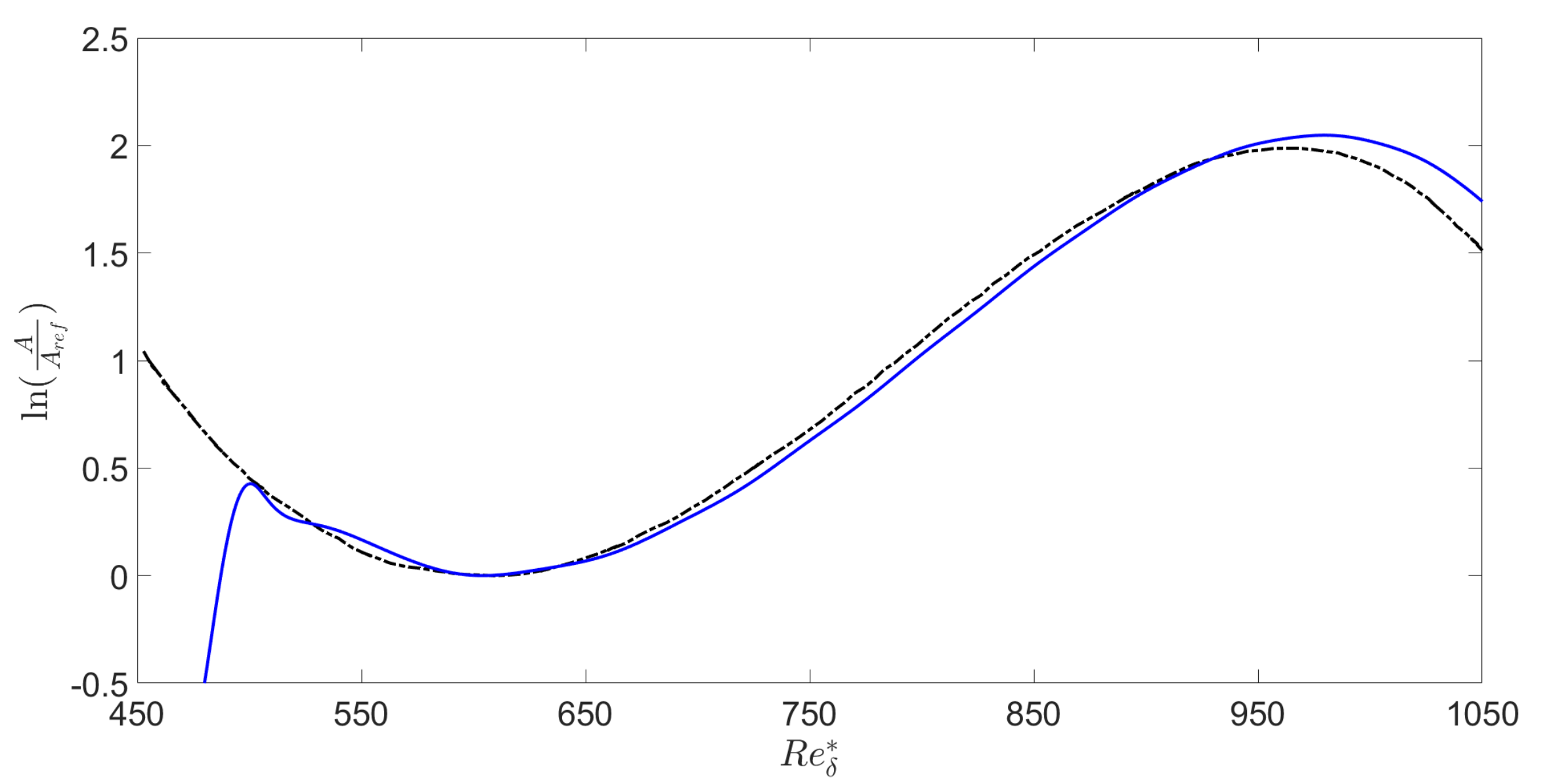
 2D DNS;
  Fasel & Konzelmann [43].
2D DNS; Fasel & Konzelmann [43].
Fasel & Konzelmann [43].
2D DNS; Fasel & Konzelmann [43].
 7th−order polynomials;
  5th−order polynomials.
7th−order polynomials; 5th−order polynomials.
5th−order polynomials.
7th−order polynomials; 5th−order polynomials.
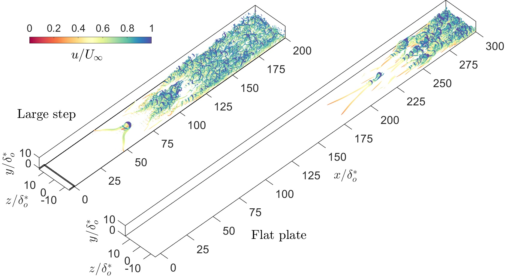
 Flat plate;
  ,
,  small step;
  ,
,  large step;
  ,
,  small step, variable . The solid line is the transitional flow, the dashed line the corresponding laminar flow.
  Turbulent correlation [42].
Flat plate; , small step; , large step; , small step, variable . The solid line is the transitional flow, the dashed line the corresponding laminar flow. Turbulent correlation [42].
Turbulent correlation [42].
Flat plate; , small step; , large step; , small step, variable . The solid line is the transitional flow, the dashed line the corresponding laminar flow. Turbulent correlation [42].
 Small step;
  small step, variable ;
  ,
,  large step.
Small step; small step, variable ; , large step.
large step.
Small step; small step, variable ; , large step.
 ;
;  . Different scales are used on x and y axes.
; . Different scales are used on x and y axes.
. Different scales are used on x and y axes.
; . Different scales are used on x and y axes.


 ;
;  .
; .
.
; .
 ;
;  .
; .
.
; .
 ;
;  .
; .
.
; .
 P;
P;  ;
;  D;
D;  C;
C;  T;
T;  ;
;  ;
;  .
P; ; D; C; T; ; ; .
.
P; ; D; C; T; ; ; .


| Case | ||||
|---|---|---|---|---|
| Flat plate | 0.0 | 0.0 | 350 × 75 × 2 | 1184 × 449 × 337 |
| Small step | 0.5 | 0.175 | 250 × 75 × 2 | 1254 × 470 × 337 |
| Large step | 1.0 | 0.350 | 250 × 75 × 2 | 1254 × 491 × 337 |
| Variable (S) | 0.5 | 0.175 | 200 × 40 × | 1590 × 393 × 169 |
| Small step (S) | 0.5 | 0.175 | 250 × 75 × | 1254 × 470 × 169 |
| Large step (S) | 1.0 | 0.350 | 250 × 75 × | 1254 × 491 × 169 |
Publisher’s Note: MDPI stays neutral with regard to jurisdictional claims in published maps and institutional affiliations. |
© 2022 by the authors. Licensee MDPI, Basel, Switzerland. This article is an open access article distributed under the terms and conditions of the Creative Commons Attribution (CC BY) license (https://creativecommons.org/licenses/by/4.0/).
Share and Cite
Teng, M.; Piomelli, U. Instability and Transition of a Boundary Layer over a Backward-Facing Step. Fluids 2022, 7, 35. https://doi.org/10.3390/fluids7010035
Teng M, Piomelli U. Instability and Transition of a Boundary Layer over a Backward-Facing Step. Fluids. 2022; 7(1):35. https://doi.org/10.3390/fluids7010035
Chicago/Turabian StyleTeng, Ming, and Ugo Piomelli. 2022. "Instability and Transition of a Boundary Layer over a Backward-Facing Step" Fluids 7, no. 1: 35. https://doi.org/10.3390/fluids7010035