Article

Improvement of a Diagnostic Urban Wind Model for Flow Fields around a Single Rectangular Obstacle in Micrometeorology Simulation

1
Marine Environment and Engine System Department, National Maritime Research Institute, National Institute of Maritime, Port and Aviation Technology, Shinkawa 6-38-1, Mitaka-shi, Tokyo 181-0004, Japan
2
Maritime Risk Assessment Department, National Maritime Research Institute, National Institute of Maritime, Port and Aviation Technology, Shinkawa 6-38-1, Mitaka-shi, Tokyo 181-0004, Japan
*
Author to whom correspondence should be addressed.
Fluids 2021, 6(7), 254; https://doi.org/10.3390/fluids6070254
Submission received: 15 June 2021 / Revised: 1 July 2021 / Accepted: 7 July 2021 / Published: 12 July 2021
(This article belongs to the Collection Feature Paper for Mathematical and Computational Fluid Mechanics)

Abstract

:
In general, computational fluid dynamics (CFD) models incur high computational costs when dealing with realistic and complicated flows. In contrast, the mass-consistent flow (MASCON) field model provides a three-dimensional flow field at reasonable computational cost. Unfortunately, some weaknesses in simulating the flow of the wake zone exist because the momentum equations are not considered in the MASCON field model. In the present study, a new set of improved algebraic models to provide initial flow fields for the MASCON field model are proposed to overcome these weaknesses by considering the effect of momentum diffusion in the wake zone. Specifically, these models for the wake region are developed on the basis of the wake models used in well-recognized Gaussian plume models, ADMS-build and PRIME. The MASCON fields provided by the new set of wake zone models are evaluated against wind-tunnel experimental data on flow around a wall-mounted rectangular obstacle. Each MASCON field is compared with the experimental results, focusing on the positions of the vortex core and saddle points of the vortex formed in the near-wake zone and the vertical velocity distribution in the far-wake zone. The set of wake zone models developed in the present study better reproduce the experimental results in both the wake zones compared to the previously proposed models. In particular, the complicated recirculation flow which is formed by the union of the sidewall recirculation zone and the near-wake zone is reproduced by the present wake zone model using the PRIME model that includes the parameterization of the sidewall recirculation zones.

1. Introduction

Predicting the three-dimensional flow fields around surface-mounted rectangular obstacles is important in applications such as urban air quality research and tracking the plumes of accidentally released toxic air pollutants. For these applications, various types of computational fluid dynamics (CFD) models have been applied to predict the flow fields around obstacles. However, CFD models have the drawback that the computational cost is substantially high.
A diagnostic mass-consistent flow (MASCON) field model is often used to predict the flow field in complex terrains [1,2,3]. The characteristics of the model are that reasonable results can be expected by using an adequate initial flow field, such as observed wind data in the model, and that the computational cost is small compared with CFD models. In the case of the dynamics of dominant flow topological features in the street canyon, the MASCON field model completed the calculation in only 5 s using a one-core processor, whereas the Reynolds average Navier-Stokes equation (RANS) model required 5 h of execution time even with four-core processors [3]. Owing to these features, the MASCON field model has been used primarily to estimate meteorology-related flow fields. However, more recently, there are some examples that have been applied to the estimate flow fields that are not directly related to meteorology, such as those used to simulate airflow around automobiles [4] or a fence-shaped obstacle [5].
The MASCON field model was developed by Röckle [6] to compute the three-dimensional flow field around surface-mounted rectangular obstacles. The model predicts flows using the mass-conservation equation in combination with empirical parametrizations to determine the initial flow fields in the upstream recirculation zone, near-wake zone, and far-wake zone of the obstacle. Following this, a mass-consistent flow field is produced by conventional diagnostic flow modeling based on a variational principle [7].
QUIC-URB is part of the Quick Urban and Industrial Complex (QUIC) dispersion modeling system containing an “urbanized” random-walk model [1]. It is based on Röckle’s MASCON field model. Singh et al. introduced additional physically based but simple parameterizations that produce vortices in front of surface-mounted rectangular obstacles and on rooftops [1]. Gowardhan et al. improved the parameterizations that produce upwind recirculation zones and rooftop flow [2]. Hayati et al. comprehensively evaluated their MASCON field model and two CFD simulations with different turbulence modeling approaches, Reynolds-averaged Navier–Stokes simulation (RANS) and large-eddy simulation (LES), against high-spatial-resolution wind-tunnel velocity data [3]. They also introduced a parametrization for sidewall-wake recirculation zones around surface-mounted rectangular obstacles [3].
MCAD, which is also based on Röckle’s MASCON field model, is a model that can calculate the flow fields in a greater variety of geometric configurations compared to the previously proposed models [8]. The model was evaluated against wind tunnel experiments for applications ranging from point-source emissions in uniform urban canopy to along-road emissions in real city geometries [8].
These models are typical algebraic models for estimating the initial flow fields of the flow around building-shaped obstacles on land. The physics and formulations of these algebraic models were well explained in various papers. However, most of the model validations were based on element tests using obstacles with a simple aspect ratio, such as cubes [2]. In addition, the MASCON fields of environments consisting of multiple obstacles simulating an urban area have been validated using the spatial concentration distributions of tracer gas from fixed emission points [8,9,10]. However, some weaknesses in the wake zone flows have been pointed out because the MASCON field model does not consider the momentum equations [11,12]. The MASCON field obtained from the Röckle model exhibits an excessively strong velocity gradient confined to a narrow area behind the surface-mounted rectangular obstacle. The stepwise change in the streamwise velocity at the wake-ambient flow interface emerges because the momentum diffusion is not modeled.
In the present study, improved algebraic models for the initial flow fields are proposed in which the effect of momentum diffusion in the wake region is considered. Each MASCON field is compared with the experimental results, focusing on the positions of the vortex core and saddle points of the vortex formed in the near-wake zone and the vertical velocity distribution in the far-wake zone. Additionally, the parameters contained in the algebraic models are improved such that the MASCON field better reproduces the experimental results compared to the conventional models.

2. The MASCON Field Model and Existing Algebraic Models for the Flow Field

2.1. The MASCON Field Model

Unlike the CFD model, the MASCON field model does not solve the Navier-Stokes equations. Instead, flow velocities are calculated from the continuity equation in such a way that the mass conservation should be met by a variational approach. The MASCON field model is a mass-consistent model that is often used for predicting the flow fields in complex three-dimensional terrain [1,2,3]. Reasonable results can be expected from the MASCON field model given an initial flow field. An initial flow field v * r , which includes the upwind and downwind recirculation zone, rooftop recirculation zone, and downwind velocity deficit, is generated on the basis of empirical parameterizations.
The initial flow field v * r most likely contains some divergences. In the case of air, these divergences must be minimized to obtain a valid flow field. After setting the initial flow field according to the parameterizations, it is necessary to obtain a velocity field v r that satisfies continuity and is as close as possible to the original field v * r . In this problem, the difference R ˜ between the initial and final velocity fields v r is minimized [7].
R ˜ = 1 2 Ω v r v * r 2 d Ω ,
where r is the position vector, and Ω is the domain over which the velocity field is defined subject to the continuity constant. Details of the MASCON field model are described in Appendix A. Some algebraic models for the initial flow fields v * r are presented in Section 2.2.

2.2. Existing Algebraic Models for the Initial Flow Fields

Typical existing algebraic models for the initial flow fields are the modified Röckle model and the shelter model, which are shown in detail below.

2.2.1. Modified Röckle Model

Most algebraic models for the diagnostic MASCON field models for calculating the three-dimensional flow field around obstacles are based on the model presented by Röckle [2]. The Röckle model utilizes empirical algorithms for the initial flow fields in the upstream recirculation, near-wake, and far-wake regions of a single obstacle (see Figure 1). Using the initial flow field, a MASCON field is calculated, similar to the approach used in traditional diagnostic flow field modeling [1]. The Röckle model makes it possible to approximate a flow field with a relatively high spatial resolution around cube- or cuboid-shaped obstacles [6,13]. After the Röckle model was proposed, various modifications were made to overcome some of the weaknesses of the model. In the present study, the Röckle model with modifications is called the modified Röckle model.
Here, the algebraic models related to the near- and far-wake zones are presented. For the upstream recirculation zone, the parametrization proposed by Gowardhan et al. [2] is used in the present study.
(1)
Rooftop recirculation zone
Gowardhan et al. [2] developed a model for the initial flow field in the rooftop recirculation zone. The length and height of the rooftop recirculation zone depend on the crosswind geometry of the obstacle. These are given with respect to the length scale R as follows:
R = B s 2 / 3 · B l 1 / 3 ,  
where B s is the smaller and B l is the larger of the obstacle height h and width w . The length l C and height h CM of the vortex in the rooftop recirculation zone are expressed as
l C = 0.9 R ,   h CM = 0.22 R .  
The following velocity parameterization [2] is used in the rooftop recirculation zone:
u ¯ z   = u 0 , z h + h CM z h CM ,
where u 0 , z is the upstream boundary layer velocity that is unaffected by the obstacle at the height z = h + h CM z .
(2)
Near-wake zone
A cavity zone, which is called the near-wake zone in the present study, is produced in the downwind of the obstacle. In the Röckle model, the near-wake zone is an ellipsoid with the length of 1 · L R downwind of the obstacle and the same width as the obstacle w [14]. In the modified near-wake zone model proposed by Fröhlich, the length L R is expressed as follows [15]:
L R h = 1.8 w / h LR l / h LR 0.3 · 1 + 0.24 w / h LR · h LR ,
where w and h are the width and height of the obstacle, respectively, and the length of the obstacle in the flow direction is specified as l . Equation (5) makes the calculation of stable values for L R possible by avoiding a large L R despite a small w through the introduction of a scaling factor h LR [15].
h LR = 5.0 · 1.0 exp 0.2 h .
The near-wake zone described in Equations (5) and (6) is confined vertically to the height of the obstacle and laterally to its width. The length of the near-wake zone d R y , z in the streamwise direction is expressed as follows [6]:
d R y , z   = L R 1 y w 2 · 1 z h 2 ,
where d R y , z is the along-wind distance measured from the downwind face of the obstacle. The following velocity parameterization is specified in the near-wake zone [6]:
u x , y , z u 0 , h = 1 x d R y , z 2 ,
where u x , y , z are the velocities at arbitrary positions in the near-wake zone, and x is the distance from the upwind face of the obstacle in the streamwise direction.
(3)
Far-wake zone
The length of the far-wake zone L w is three times that of the near-wake zone L R in Equation (5) [6].
L w = 3 L R .
The length of the far-wake zone d w y , z is the along-wind distance from the downwind face of the obstacle and is expressed as follows [6]:
d w y , z   = L w 1 y w 2 · 1 z h 2 .
Within the far-wake zone L R < x < 3 · L R , the following velocity parameterization is specified [6]:
u x , y , z u 0 , z = 1 d w y , z x 1.5 .

2.2.2. Shelter Model

The MASCON field obtained from the modified Röckle model exhibits an excessively strong velocity gradient confined to a narrow area behind the obstacle [11,12]. This stepwise change in the streamwise velocity observed at the wake–ambient flow interface emerges because the momentum diffusion is not modeled. To overcome this issue, an algebraic model that implements the momentum diffusion mechanism based on the shelter model [16] was proposed [8,11,12]. The shelter model produces a Gaussian velocity deficit profile in the wake zone using the following equations [16]:
u d x , y , z u 0 , h = Γ C D ˜ w h · x h 1.5 F η G ζ ,
F η   = 1 2 π a f exp η 2 2 a f 2 ,
G ζ   = c a ζ exp a g ζ 1.5 .
In the above equations, u d x , y , z is the velocity deficit at the arbitrary positions x , y , z in the wake zone, and w and h are the width and height of the obstacle, respectively. Γ and C D ˜ = 0.2 + 0.35 / 2 [8] are the drag coefficients. Γ is empirically expressed as follows [16]:
Γ = 0.67 C a 2 .
The functions F η and G ζ are the lateral and vertical velocity deficit variations, respectively [16].
η = y h x h 1 / 2 , ζ = z h x h 1 / 2 .
The coefficient a f is the lateral wakespread parameter. The vertical coefficients c a and a g are defined as follows [16]:
c a = ln h + z 0 z 0 2 κ 2 ,
a g = 0.67 C a 1.5 ,
where z 0 is the aerodynamic roughness, and κ is the von Kármán constant (0.4).
Note that the shelter model applies only to the downstream region, including the near-wake and far-wake zones in the Röckle model. The shelter model does not include the parametrization of the near-wake and rooftop recirculation zones and the velocity parameterization in these zones. In the present study, the velocity parameterization in the zones proposed by Röckle in Equations (2)–(8) is incorporated into the shelter model.
The results of the MASCON field using the modified Röckle and shelter models are shown in Section 4, together with the results obtained using the algebraic model proposed in the present study. As described later, the MASCON field based on the existing algebraic models does not adequately reproduce the experimental results in the near- and far-wake zones.

3. Methodology

3.1. Improved Algebraic Models for Flow Fields Using MASCON Field Model

The MASCON field based on existing algebraic models inadequately reproduces the experimental results in the near- and far-wake zones. In the present study, two algebraic models are proposed to resolve the issues associated with these existing models. The flow field estimation schemes used in the two different plume models are improved for use as algebraic models in the MASCON field.

3.1.1. ADMS-Build Wake Model

The ADMS-build wake model is a module in the urbanized version of the Gaussian plume-dispersion model ADMS [17,18,19]. The ADMS building effects module calculates the near-field dispersion of pollution from sources close to large buildings or groups of buildings represented as a single effective building. In the module, a simplified flow field is defined on the basis of a well-mixed cavity or recirculating flow region and a downstream wake region with reduced momentum.
The ADMS-build wake model is applicable only when U > 0 , i.e., downwind of the near-wake zone where x is larger than L R (see Figure 2). L R is determined by the along-wind length l , crosswind width w , and height h of the obstacle as follows [17]:
L R = A w 1 + B w / h ,   B = 0.24 , A = 1.8 l h 0.3 , 0.3 < l h < 3 .
Note that, if w / h is small, L R A w .
The upper limit of the near-wake zone z R x is as follows [17]:
z R x   = z Rmax 1 x x Rmax x R x Rmax 2 ,
z Rmax = h ,   x sep = l 2 ,      l min h , 0.5 w , z Rmax = h · 1 + 0.7 1 exp w 2 l h ,   x sep = l 2 , l < min h , 0.5 w
where x sep is the downwind rooftop separation point. In the ADMS-build model, the length L R of the near-wake zone is given by Equations (19)–(21), whereas no parameterizations are provided for the rooftop and near-wake zones. In the present study, the parameterization for each zone proposed by Röckle represented by Equations (2)–(8) is applied for the zone in the ADMS-build model. Equation (7) can be expressed as
d R y , z   = L R 1 y w 2 · 1 z z Rmax 2 .
The flow components in the far-wake zone are as follows [17]:
u = u 0 , h · 1 u ^ · w 2 l y · h l z 2 · p ξ · q η , v = u 0 , h · u ^ · w 2 x x 0 · h l z 2 · p ξ · η 2 · q η , w = u 0 , h · u ^ · h x x 0 · w 2 l y · h l z · g ξ ξ = 0 g ξ · q η .
The normalized crosswind dimensions η and ξ are expressed as follows using the length scale l y , z x [17]:
η = y l y ,       ξ = z l z ,
l y , z x   = D y , z · x x 0 u 0 , h ,
where D y , z are the constant eddy viscosities under neutral conditions [17].
D y = κ · u * · h ,       D z = 2 · κ · u * · h .
The virtual origin x 0 in Equation (25) is defined such that u > 0 throughout the main wake. The velocity perturbation parameter u ^ is assumed to be 0.45, as given in the literature [17]. The shape functions p ξ and q η are defined as follows [17]:
p ξ   = ξ 2 · exp ξ 2 4 ,       q η = 1 2 π · exp η 2 4 .
As shown in Figure 2, the boundary between the near- and far-wake zones of the ADMS-build model is the yz plane perpendicular to the x-axis, where u > 0 . In the region downstream from the downwind face of the obstacle, the inside of the near-wake zone contains a negative velocity ( u < 0 ), whereas u > 0 outside the 1/4 ellipsoid that defines the near-wake zone. In the present study, the boundary of the far-wake zone is extended to the outer surface of the 1/4 ellipsoid that delineates the near-wake zone (red line in Figure 2). The modified model is called the ADMS-build model in the present study.

3.1.2. PRIME Model

Similar to the ADMS model, the PRIME model [20] is a Gaussian dispersion model. The PRIME model incorporates building downwash effects, including enhanced dispersion in the wake, reduced plume rises due to streamline deflection and increased turbulence, and continuous treatment of the near- and far-wake zones. The model can estimate the position of the stack relative to the obstacle, the streamline deflection near the obstacle, and the shear of the vertical flow and velocity deficit (see Figure 3).
In the PRIME model, the length scale in Equation (2) is used to estimate the rooftop recirculation zone. The value used for B l is restricted to 8 B s [21]. When l > 0.9 R , the rooftop recirculation zone reattaches to the obstacle, and the maximum height of the near-wake zone h R is as follows [22]:
h R = h .
When l 0.9 R , the rooftop recirculation zone does not reattach, and h R is given as follows [20]:
h R x   = h + 0.22 R   at   x = 0.5 R ,
where x is the along-wind distance measured from the upwind face of the obstacle. The height and width of the near-wake envelope h C x ,   w C x are as follows [20]:
h C x   = h     0 x l , h C x   = h · 1 x l L R 2     l x l + L R , h C x   = h R + 4 x R / 2 2 · H h R R 2     0 x R / 2 , h C x   = h R · 1 x R / 2 l + L R R 2       R / 2 x L R .
The horizontal boundary of the near-wake zone w C x is estimated using the following equation on the basis of the analysis of horizontal-plane streamlines in a wind tunnel experiment by Snyder and Lawson [23]:
w C x   = w 2 + R 3 x R 2 3 R     0 x R , w C x   = w 2 + R 3 · 1 x R l + L R R 2       R x l + L R .
In the present study, the envelope height is assumed to be
h C x   = h R .
The parameterizations for the rooftop recirculation zone and near-wake zone in Equations (2)–(8) proposed by Röckle are also applied as the zones of the PRIME model. Equation (7) can be expressed as
d R y , z   = L R 1 y w C x 2 · 1 z h C x 2 .
The wake boundary, h w x ,   w w x , is also based on the analysis of the horizontal-plane streamlines in a wind-tunnel experiment [20,22].
h w x   = 1.2 R · x R + h 1.2 R 3 1 / 3 , w w x   = w 2 + R 3 · x R 1 / 3 .
These equations indicate the x 1 / 3 dependence of the three-dimensional far-wake growth.
In the present study, the velocity parameterization proposed by Röckle for the far-wake zone in Equations (10) and (11) is applied to the far-wake zone of the PRIME model. Equation (10) can be expressed as
d w y , z   = L R 1 y w w x 2 · 1 z h w x 2 .
The sidewall recirculation zones (see Figure 3) are generated on both sidewalls of the obstacle, which were parameterized by Hayati et al. [3]. At the vertical levels where the side-bubble zones exist, the vortex is defined similarly to the rooftop vortex that develops along the upwind edge of a flat roof and is nominally perpendicular to the prevailing flow direction [3]. In the present study, sidewall recirculation zones are incorporated into the PRIME model. The downwind length l C and lateral width w C of the elliptical recirculation region in the sidewall recirculation zones are expressed as
l C = 0.9 R ,      w C = 0.22 R ,
where R is the vortex size scaling factor defined in Equation (2), and the lateral width w C is also the height of the vortex. In the present study, the following velocity parameterization is specified in the sidewall recirculation zones:
u ¯ y , z   = u 0 , z w + w C y w C ,
where u 0 , z is the upstream boundary layer velocity that is unaffected by the obstacle at z . The model with the above modifications is called the PRIME model in the present study.

3.2. Wind-Tunnel Measurement Data

The physics and formulation of some MASCON field algebraic models are well explained in various research papers. These models were validated on the basis of element tests using obstacles with simple aspect ratios, such as cubes [2]. In other models, the MASCON fields of environments consisting of multiple obstacles simulating an urban area were validated using the spatial concentration distribution of tracer gas from a fixed emission point [8,9,10]. The existing studies, however, did not investigate the environments in which the MASCON field based on algebraic models is applicable. The characteristics and limitations of the models should, therefore, be discussed from various perspectives. In the present study, the MASCON fields obtained from the algebraic models are compared with the results of two wind tunnel experiments, namely, the measurements of Wang et al. [24], who obtained information on the vortex and flow velocity around obstacles, and those of Meng et al. [25], who measured the vertical velocity profile with respect to the flow direction from the upwind face of the obstacle. These wind-tunnel experiments were selected according to their applicability for the near-wake and far-wake zones.

3.2.1. Outline of the Experiment by Wang et al. and Computational Condition

In the experiment by Wang et al. [24], the three-dimensional turbulent wake flow around different building models was measured using time-resolved particle-image velocimetry (PIV). The mean flow streamlines, velocity component, turbulent kinetic energy, Reynolds shear stress distribution, and positions of the saddle points and vortex cores in the wake were evaluated for flow fields around obstacles. The Reynolds number based on the obstacle width w and mean free stream flow velocity at the roof U H ¯ was 2.16 × 10 4 . The time-resolved flow field was measured using PIV on the horizontal and vertical planes of the obstacle. PIV measurements were performed on several horizontal planes at various distance intervals with the central vertical plane located at y / H = 0 .
The inflow conditions used in the present study were obtained from the mean velocity profile and turbulence intensity. The logarithmic law of the velocity distribution for neutral atmospheric stability is given by
u u * = 1 κ · ln z z 0 .
In the present study, the friction velocity and surface roughness were, respectively, obtained as u * = 0.281 m/s and z 0 = 5.50 × 10 5 m as a function of z = 0.12 m. The MASCON fields based on each algebraic model were obtained using the above inflow conditions. The domain size used for the calculations was set to 10 l in the mainstream direction, 7 l across the flow direction, and 8 l in the vertical direction, where l is the length of the obstacle (see Figure 4). According to Singh et al. [1], the calculation of the MASCON field based on the modified Röckle model requires a uniform grid resolution in which the cubic-shaped obstacle l is resolved with at least 10 cells in each direction. With this in mind, the domain size used was 100 × 70 × 80 = 560,000 in grid cell units.

3.2.2. Outline of the Experiment by Meng et al. and Computational Condition

The Working Group of the Architectural Institute of Japan (AIJ) has published guidelines [26] on CFD techniques for the prediction and assessment of the pedestrian wind environment around buildings. The guidelines consist of a cross-comparison among CFD predictions, wind-tunnel test results, and field measurements, which are used to investigate the influence of some of the computational conditions for various flow fields. In the present study, the test case for a square prism with the aspect ratio of l : w : h = 1 : 1 : 2 was adopted. Meng et al. [25] conducted an experiment on the test case. The Reynolds number based on the obstacle width w and mean free stream flow velocity at the roof U H ¯ was 2.4 × 10 4 . The mean flow velocity was measured for each component using a split-fiber probe. The measurement was performed on the y / b = 0 vertical cross-section and the horizontal cross-section at 10 / 16 of the building height ( z / b = 1.25 ).
In the present study, the friction velocity and surface roughness were, respectively, obtained as u * = 0.293 m/s and z 0 = 4.49 × 10 5 m as a function of z = 0.16 m. The MASCON fields based on each algebraic model were obtained using the inflow conditions above. The domain size used for the calculations was set to 10 l in the mainstream direction, 7 l across the flow direction, and 8 l in the vertical direction using the length l of the obstacle, as described in Section 3.2.1 (see Figure 4); the domain size was 100 × 70 × 80 = 560,000 in grid cell units.

4. Results and Discussion

The MASCON fields obtained from the algebraic models were compared with the experimental results. The experimental results obtained by Wang et al. [24] and Meng et al. [25] were used for the evaluation. Each MASCON field was obtained by the minimal adjustment of the initial flow fields represented by a series of the algebraic models, as shown in Appendix A of this paper. The program of the MASCON field model shown in Appendix A was coded by Fortran 90.

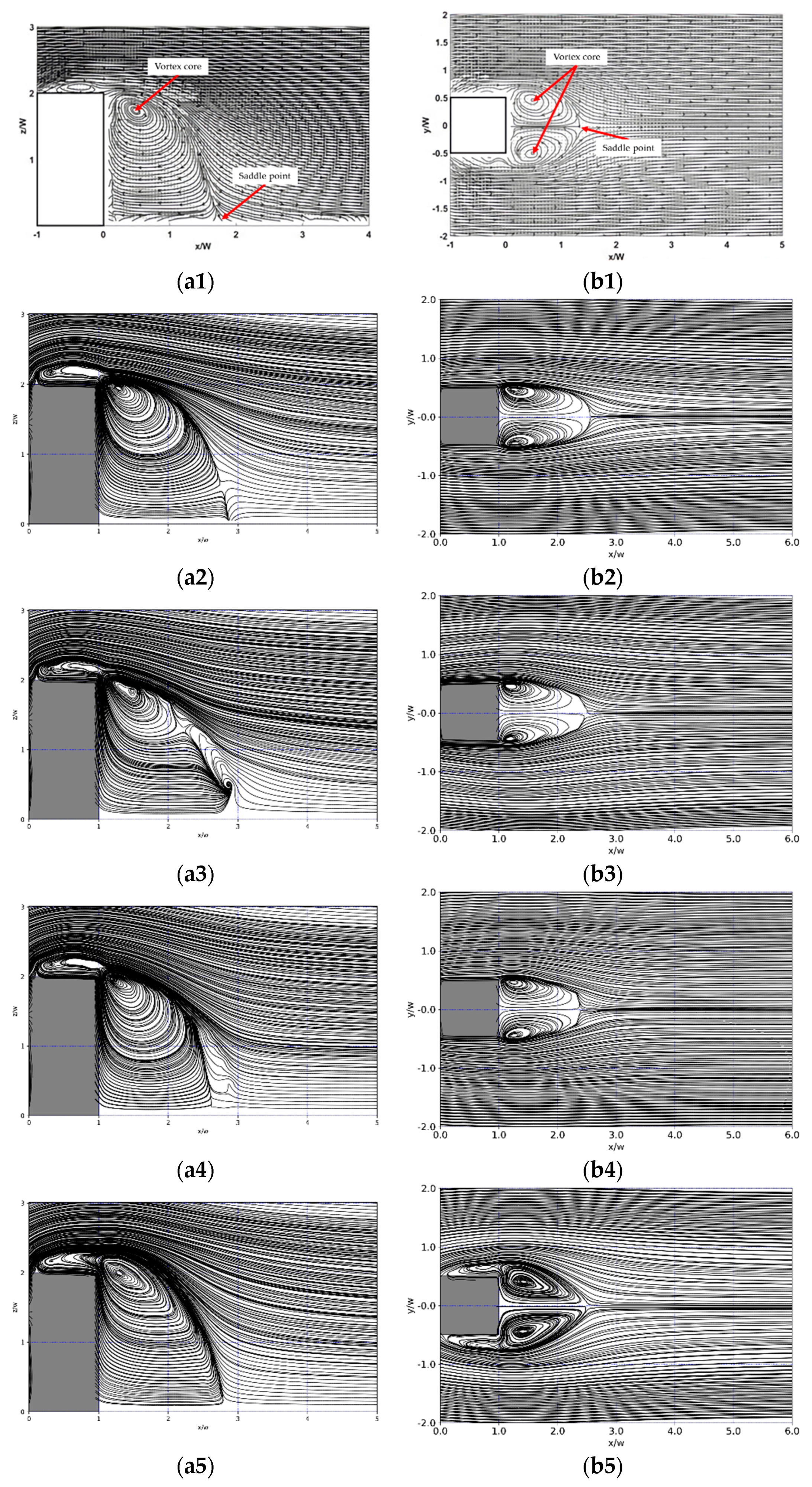
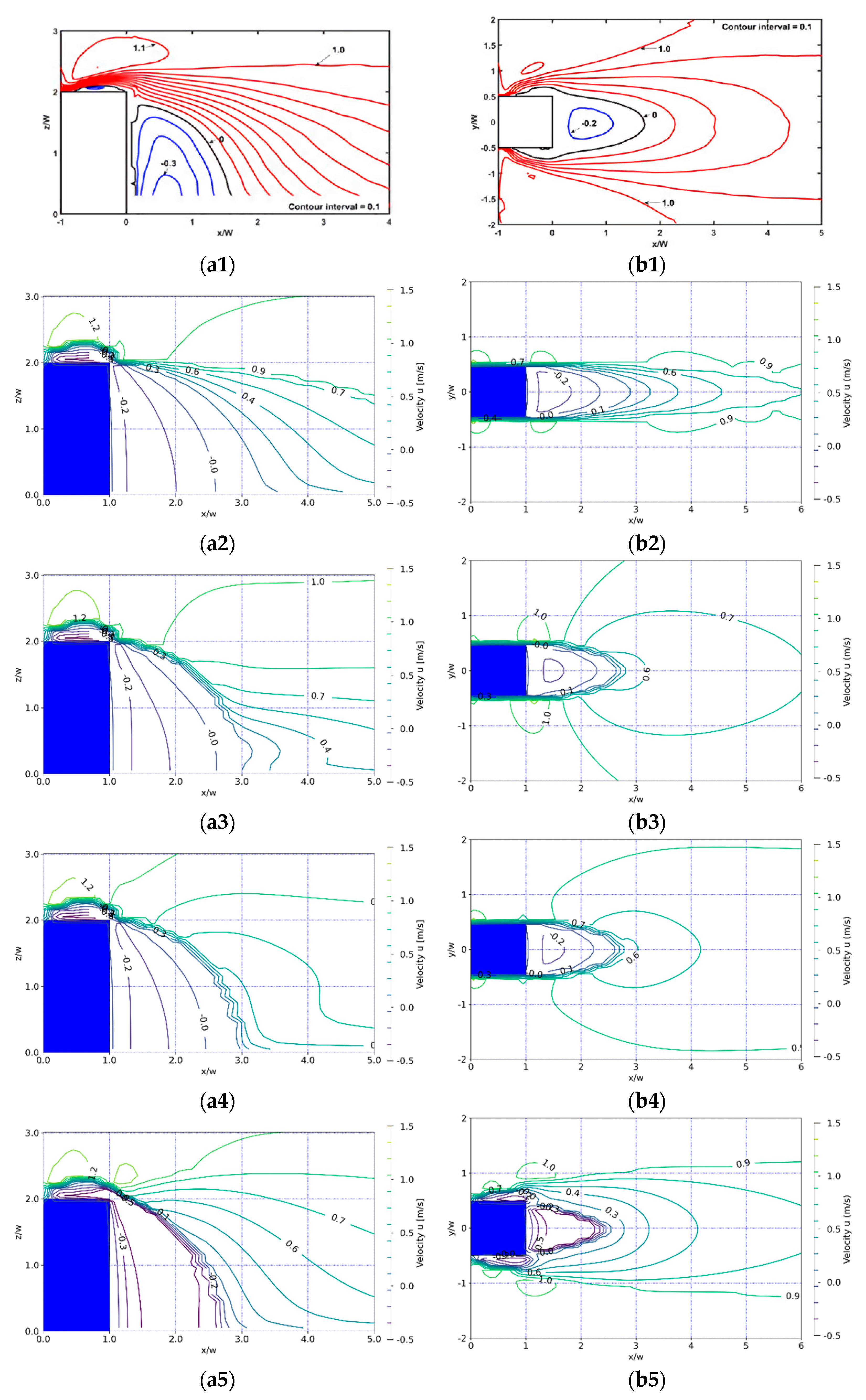
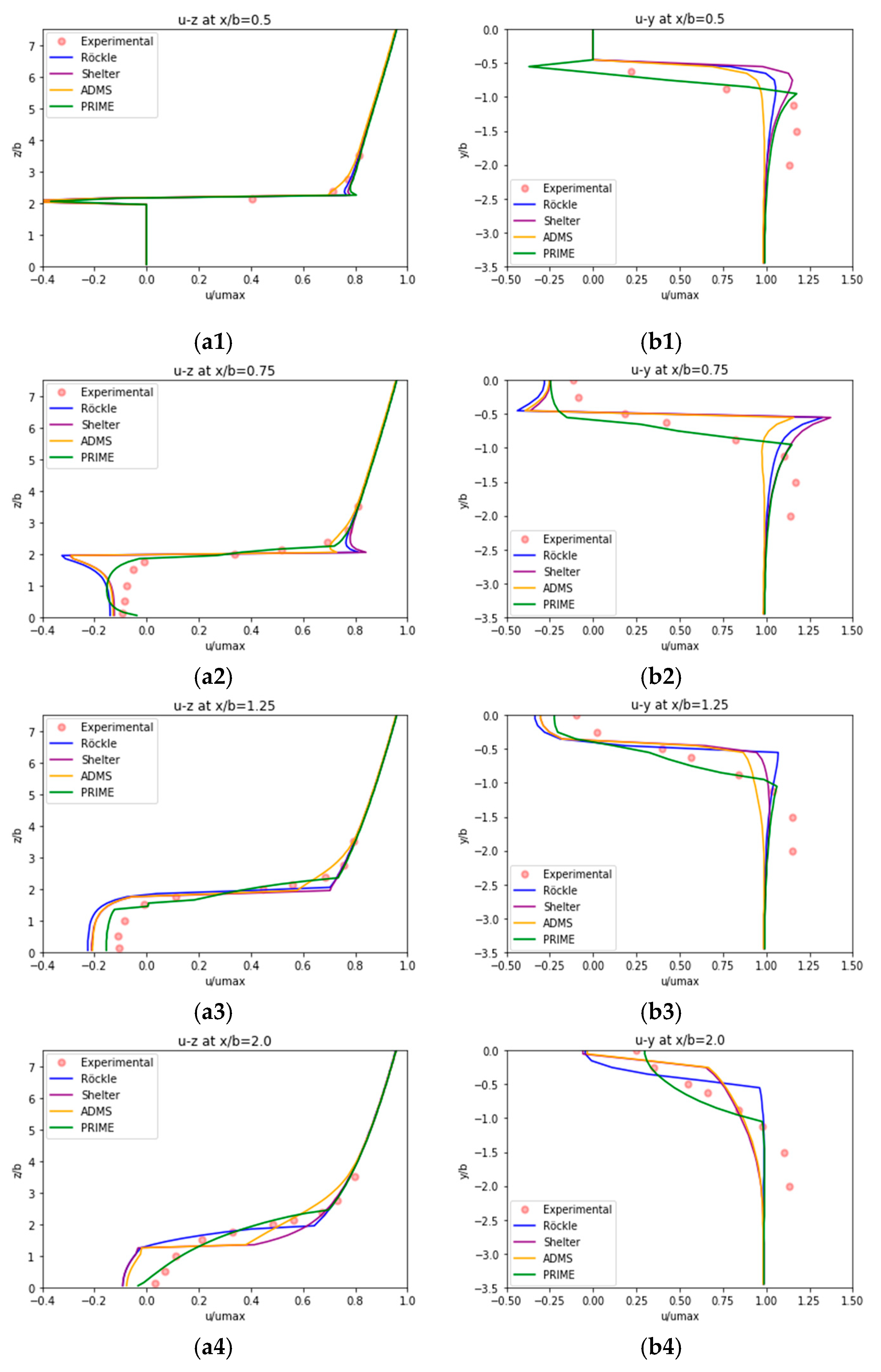
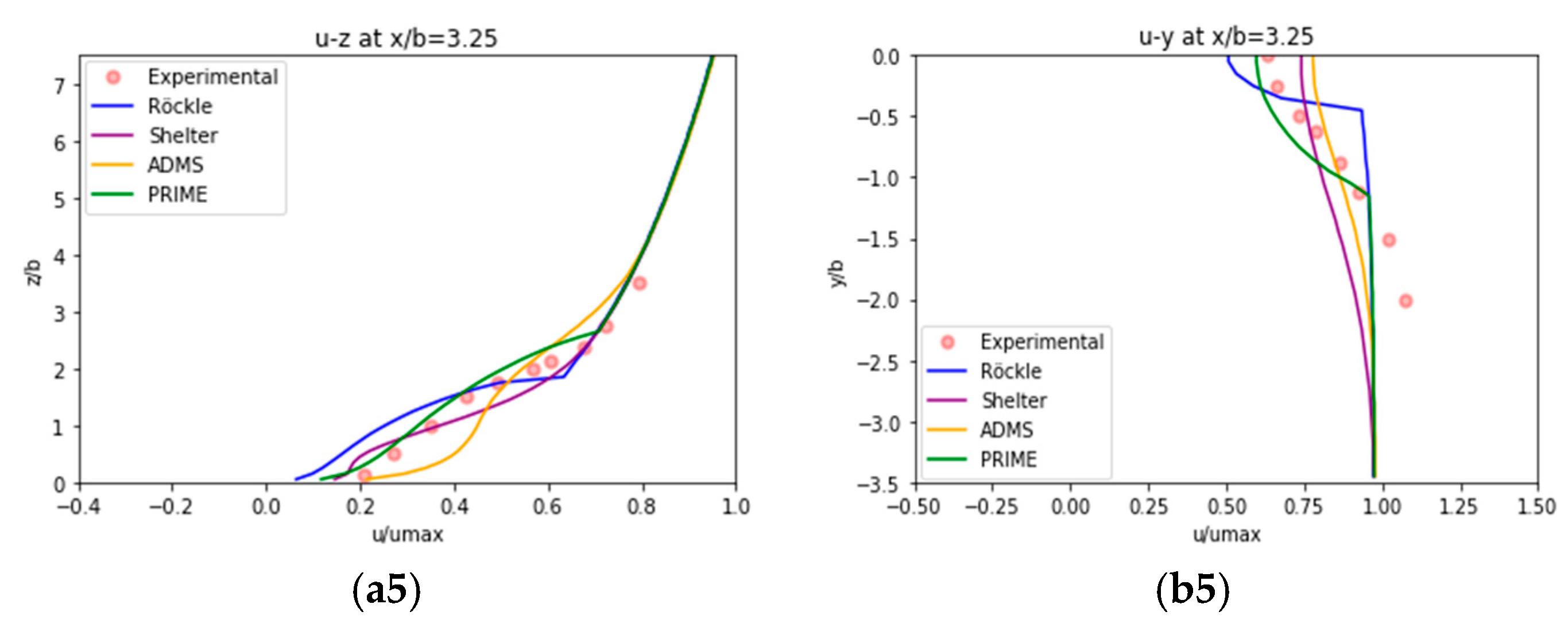
4.1. Comparison with Experiment by Wang et al.

Figure 5(a1,b1) show the streamlines obtained from the experiment by Wang et al. [24] representing the flow fields on the symmetry plane at y = 0 and on the mid-height horizontal plane around the obstacle at z = h / 2 , respectively. The general wake pattern behind an obstacle is characterized by recirculating flow. The near-wake zone behind the obstacle is one of the regions where recirculating flow occurs. As shown in Figure 5(a1), a distinct recirculating flow occurs in the near-wake zone behind the object. In Figure 5(b1–b5), it can be seen that two recirculating flows occur in the near-wake zone. Note the slight extension of the recirculation flows on the horizontal plane slightly beyond the width of the obstacle and the presence of other circulations that flow near both sides of the obstacle.
Figure 5(a2–a5,b2–b5) show the streamlines of the MASCON field obtained from the various algebraic models. The streamlines obtained from all the algebraic models exhibit a recirculating flow in the rooftop and near-wake zones. In the ADMS-build and PRIME models, the boundary of the rooftop recirculation flow changes according to the obstacle aspect ratio (see Equations (19), (21), (30) and (31)). The rooftop recirculation zone does not reattach to the rooftop of the obstacle only in the PRIME model. As a result of the increased correlation between each zone, the MASCON field from the PRIME model has a recirculation flow in the region where the two zones are fused. From Figure 5(a5,b5), it was confirmed that the rooftop recirculation zone does not reattach to the downstream side on the rooftop of the obstacle in agreement with the experimental result. The boundary of the near-wake zone obtained from the shelter model was ambiguous compared to that of the other models (see Figure 5(a3)). This is because the initial velocity field given to the near-wake zone in the 1/4 ellipsoidal shape interfered with the flow of the far-wake zone given by the shelter model.
It is worth noting that the streamlines in Figure 5(b5) obtained from the PRIME model reproduced the experimentally obtained circulation flows that extended slightly beyond the width of the obstacle. In addition, the recirculations in the sidewall recirculation zones also reproduced the experimental results well because the initial flow field associated with the sidewall recirculation zones was incorporated into the PRIME model (see Equations (36) and (37)). These features are some of the advantages of the PRIME model.
The recirculation flow is generally characterized by the locations of the vortex cores and saddle points in the near-wake zone. The locations of the saddle points and vortex cores of the recirculation flow inside the near-wake zone obtained by the MASCON field model were compared with the experimental results. The locations of the saddle points and vortex cores in the near-wake zone could be identified from the streamlines in Figure 5 and are summarized in Table 1. Comparing the MASCON field with the experiment, the distance of the vortex core from the back of the object x vc / w was smaller, and the height from the floor z vc / w was larger. The locations of the saddle points were almost in agreement with the experimental results. Examining the various algebraic models, the PRIME model fully reproduced the experimental location for the saddle point x sp / w . In comparison, the locations of the vortex core and the saddle point in the ADMS model deviated from the experimental results while the saddle points were indistinct in the shelter model. In summary, it can be concluded that the MASCON fields from the PRIME model are a good model for near-wake zone, although they are not superior in all cases.
The contours of the velocity component u obtained from the experiment by Wang et al. [24] on the obstacle symmetry plane at y = 0 and the obstacle mid-height horizontal plane at z = h / 2 are shown in Figure 6(a1,b1), respectively. As shown in Figure 6(a2–a5,b2–b5), the velocity distributions in the far-wake zone downstream of the near-wake zone differed significantly between the models. In the modified Röckle model, the formation range of the far-wake zone was constrained by a 1/4 ellipsoid, and the ambient flow velocity was given only on the outside of the ellipsoid (see Equations (9)–(11)). This indicates that the modified Röckle model provides an initial flow field with a large velocity difference at the boundary of the elliptical plane. The MASCON field obtained from such an algebraic model inadequately reproduced the experimental results. The effect of momentum diffusion could be confirmed in the contour diagram obtained by replacing the far-wake zone of the modified Röckle model with the shelter model (see Figure 6(a3,b3)). However, the calculation results did not quantitatively reproduce the experimental results. Velocity distributions close to the experimental results were obtained from the ADMS-build (Figure 6(a4,b4)) and PRIME models (Figure 6(a5,b5)). These new models provided a better estimate of the velocity transition in the wake region compared to the results of the modified Röckle and shelter models.

4.2. Comparison with Experiment by Meng et al.

The calculation results for the MASCON fields based on the algebraic models were evaluated by comparison with the experimental results of Meng et al. [25]. In the present study, the experimental results from the end of the obstacle to the downstream were used for comparison with the calculation results. The normalized vertical and horizontal velocity profiles of the velocity component u were plotted at several distances downstream of the obstacle as shown in Figure 7, where u max , the velocity in the undisturbed flow, was 6.75 m/s at z / b = 7.5 for the vertical profiles and 4.02 m/s at y / b = 1.25 for the horizontal profiles. The modified Röckle model exhibited an excessively strong velocity gradient confined to a narrow area behind the obstacle because the effect of momentum diffusion was not considered. The MASCON fields obtained from the shelter and ADMS-build models, which incorporate the effect of momentum diffusion, still exhibited steep velocity gradients at the building height at z / b = 2 . This indicates that the effect of momentum diffusion is insufficient around the near-wake zone.
The location x / b = 0.5 in Figure 7(a1,b1), which was just behind the obstacle, could be identified as the transition boundary between the rooftop recirculation zone and the near-wake zone. The obstacles used in the experiment by Meng et al. had the aspect ratio of 1:1:2. For the obstacle aspect ratio of 1:1:2 in the PRIME model, the boundary surface of the rooftop recirculation zone did not reattach to the downstream side of the obstacle rooftop. In other words, the rooftop recirculation zone and near-wake zone were merged. Figure 7(a5,b5) show that the PRIME model was superior to the other models in reproducing the experimental values in the horizontal section.
The locations included in the near-wake zone were x / b = 0.75 and 1.25 because Meng et al. found that the location of the saddle point in the near-wake zone was approximately x / b = 1.92 in the experiment [25]. As shown in Figure 7(a2,a3,b2,b3), there were remarkable differences between the models. In the MASCON field from the Röckle model, there was a velocity discontinuity at z / b = 2 near the rooftop of the obstacle in the vertical section velocity distribution and at y / b = 0.5 near the side surface in the horizontal section velocity distribution. The MASCON fields obtained from the shelter and ADMS-build models had steep velocity gradients at the building height at z / b = 2 and at y / b = 0.5 . In the MASCON field from the PRIME model, the velocity changed continuously in the approximate transition region located within the range of z / b = 1.75 - 2.25 near the rooftop of the obstacle and y / b = ± 0.5 - 1.0 near the side surface. The MASCON field obtained from the PRIME model reproduced the experimental results very well compared to the other models owing to the effect of momentum diffusion. In the PRIME model, not only was the effect of momentum diffusion properly reflected in the MASCON field, but the velocity change at the height of the obstacle also reproduced the experimental results.
As shown in the profiles in Figure 7(a4,a5,b4,b5) for x / b = 2.0 and 3.25 , which were located in the far-wake zone away from the near-wake zone, the difference between the experimental results and the results from all the models except the PRIME model increased as the distance from the back of the obstacle increased. In the PRIME model, the experimental results were reproduced very well in the regions corresponding to these far-wake zones.
In the modified Röckle model, the far-wake zone was defined by a 1/4 ellipsoid that extended the near-wake zone to the downstream direction, resulting in a steep velocity gradient on the ellipsoidal surface. Considering that momentum diffusion is one method to overcome this defect, in the MASCON field using the shelter model, the velocity distribution in the far-wake zone insufficiently reproduced the experimental results. It is shown that, using the PRIME model proposed in the present study, the MASCON field could reproduce the experimental results well not only in the near-wake zone, but also in the far-wake zone velocity field.

5. Concluding Remarks

The MASCON field model provides a three-dimensional flow field at a low computational cost, which is very useful for predicting realistic and complicated flow fields for applications such as environmental risk assessments. However, some weaknesses in the flow of the wake zone exist because the momentum equations are not considered in the MASCON field scheme. The MASCON field obtained using the shelter model, which is a typical algebraic model for considering momentum diffusion, insufficiently reproduced the experimental results in the wake zone.
In the present study, an algebraic model in the wake zone to provide the initial velocity for the MASCON field model was developed on the basis of the wake models implemented in two well-recognized Gaussian plume models, ADMS-build and PRIME. The conclusions are summarized as follows:
  • The new set of wake zone models based on ADMS-build and PRIME wake models can provide the initial velocity in the near-wake zone and take into consideration the effect of momentum diffusion in the far-wake region.
  • Streamlines obtained from the experiment around the obstacle representing the flow field on the mid-height horizontal plane show the complicated recirculation flow formed by the union of the sidewall recirculation zone and the near-wake zone. The present wake zone model based on the PRIME model that includes the parameterization of the sidewall recirculation zones can reproduce such a recirculation flow.
  • In the far-wake zone, the flow fields according to the present models considering the effect of momentum diffusion are all in general agreement with the experimental results. In particular, the wake zone model based on the PRIME model provides the excellent flow field that precisely reproduces the profile of the vertical velocity distribution of the experimental results.
Therefore, these findings suggest that the MASCON field provided by the wake zone model based on the PRIME model proposed in the present study best reproduces the entire flow field from relatively close to the obstacle to the downstream.

Author Contributions

Conceptualization, M.A. and H.O.; methodology, M.A., A.K. and H.O.; formal analysis, M.A.; resources, M.A., A.K. and H.O.; writing—original draft preparation, M.A.; writing—review and editing, A.K. and H.O.; supervision, H.O.; project administration, H.O.; funding acquisition, M.A. All authors have read and agreed to the published version of the manuscript.

Funding

This work was supported by JSPS KAKENHI (Grant Number JP16K00580).

Institutional Review Board Statement

Not applicable.

Informed Consent Statement

Not applicable.

Data Availability Statement

Not applicable.

Conflicts of Interest

The authors declare no conflict of interest.

Appendix A

The initial flow field v * r most likely contains several divergences because it does not satisfy the law of conservation of mass. It is necessary to obtain a velocity field v r that satisfies the continuity and is as close as possible to the original field v * r . In this problem, the difference R ˜ between the initial and final velocity fields v r is minimized, as shown in Equation (1). The velocity field is defined over, subject to the continuity constant being satisfied everywhere in the field [27].
· v r   = 0
A way of dealing with the problem of calculus of variations is to introduce a Lagrange multiplier, λ r . This is replaced by the problem of minimizing Equation (A1).
R = 1 2 Ω v r v * r 2 d Ω Ω λ r · v r d Ω .
Suppose that the function that minimizes the functional R is v r , where v r also satisfies Equation (A1).
R min = 1 2 Ω v r v * r 2 d Ω .
If R min is a true minimum, then any deviation from v r must produce a second-order change in R . Thus, suppose that
v = v r + δ v ,
where δ v is small but arbitrary. Substituting v into Equation (A3) yields the result R min + δ R . δ R is expressed as follows:
δ R = 1 2 Ω δ v r · v r v * r d Ω Ω λ r · δ v r d Ω .
Here, the term of second order δ v 2 has been dropped in the above equation. Integrating the last term by parts and applying Gauss’s theorem, the following equation is obtained:
δ R = 1 2 Ω δ v r · v r v * r + λ r d Ω S λ r δ v r · n d S .
On the domain surface on which a boundary condition such as walls or inflow on v is given, it is presumed that both v and v satisfy the given condition. Hence, δ v is zero there. No condition on λ is required on them because these portions of the boundaries make no contribution to the surface integral Equation (A6).
On the boundary where other types of boundary conditions such as symmetry planes or outflows are given, δ v is not necessarily zero. To make the surface integral vanish, λ = 0 is required on the boundary. If δ R is to vanish for arbitrary δ v , it is required that the volume integral in Equation (A6) also vanishes. Therefore,
v r v * r + λ r   = 0 .
Since v r satisfies the continuity Equation (A1), taking the divergence of the equation and applying this condition yields
Δ λ r   = · v * r .
The above equation is a Poisson equation for λ r . On those portions of the boundary on which boundary conditions are given on v , v = v * . In this case, Equation (A7) is λ r = 0 , which is a boundary condition on λ . If Equation (A8) is satisfied with the boundary conditions, the velocity field is divergence-free. The modified velocity field is obtained from the Equation (A7) written in the following form by solving the Poisson equation:
v r   = v * r λ r .
This show that the Lagrange multiplier λ r essentially plays the role of pressure. The function of pressure is to allow continuity to be satisfied in incompressible flows.

References

  1. Singh, B.; Hansen, B.; Brown, M.J.; Pardyjak, E.R. Evaluation of the QUIC-URB fast response urban wind model for a cubical building array and wide building street canyon. Environ. Fluid. Mech. 2008, 8, 281–312. [Google Scholar] [CrossRef]
  2. Gowardhan, A.A.; Brown, M.J.; Pardyjak, E.R. Evaluation of a fast response pressure solver for flow around an isolated cube. Environ. Fluid Mech. 2010, 10, 311–328. [Google Scholar] [CrossRef]
  3. Hayati, A.N.; Stoll, R.; Kim, J.J.; Harman, T.; Nelson, M.A.; Brown, M.J.; Pardyjak, E.R. Comprehensive Evaluation of Fast-Response, Reynolds-Averaged Navier–Stokes, and Large-Eddy Simulation Methods Against High-Spatial-Resolution Wind-Tunnel Data in Step-Down Street Canyons. Bound.-Layer Meteorol. 2017, 164, 217–247. [Google Scholar] [CrossRef]
  4. Kimura, A.; Asami, M.; Oka, H.; Oka, Y. Development of an Algebraic Model of Empirical Parameterization of Near Wakes around a Vehicle. Fluids 2021, 6, 75. [Google Scholar] [CrossRef]
  5. Peña, A.; Bechmann, A.; Conti, D.; Angelou, N. The fence experiment—Full-scale lidar-based shelter observations. Wind Energ. Sch. Discuss. 2016, 1, 101–114. [Google Scholar] [CrossRef] [Green Version]
  6. Röckle, R. Bestimmung der Stomungsverhaltnisse im Bereich Komplexer Bebauugsstruckturen. Ph.D. Thesis, Vom Fachbereich Mechanik, der Technischen Hochschule Darmstadt, Darmstadt, Germany, 1990. [Google Scholar]
  7. Sherman, C.A.A. Mass-Consistent Model for Wind Fields Over Complex Terrain. J. Appl. Meterol. 1978, 17, 312–319. [Google Scholar] [CrossRef] [Green Version]
  8. Kanda, I.; Yamao, Y.; Ohara, T.; Uehara, K. An Urban Atmospheric Diffusion Model for Traffic-Related Emission Based on Mass-Conservation and Advection-Diffusion Equations. Environ. Model Assess. 2013, 18, 221–248. [Google Scholar] [CrossRef]
  9. Brown, M.J.; Williams, M.D.; Nelson, M.A.; Werley, K.A. QUIC Transport and Dispersion Modeling of Vehicle Emissions in Cities for Better Public Health Assessments. Environ. Health Insights 2015, 9, 55–65. [Google Scholar] [CrossRef] [PubMed]
  10. Hanna, S.; White, J.; Trolier, J.; Vernot, R.; Brown, M.; Gowardhan, A.; Kaplan, H.; Alexander, Y.; Moussafir, J.; Wang, Y.; et al. Comparisons of JU2003 observations with four diagnostic urban wind flow and Lagrangian particle dispersion models. Atmos. Environ. 2011, 45, 4073–4081. [Google Scholar] [CrossRef]
  11. Pardyjak, E.R.; Brown, M.J.; Bagal, N. Improved Velocity Deficit Parameterizations for a Fast Response Urban Wind Model. In Proceedings of the 84th AMS Annual Meeting, Seattle, WA, USA, 10–16 January 2004. [Google Scholar]
  12. Singh, B.; Pardyjak, E.R.; Brown, M.J. Testing of a Far-wake Parameterization for a Fast Response Urban Wind Model. In Proceedings of the 6th AMS Urban Environment Symposium, Atlanta, GA, USA, 28 January–3 February 2006. [Google Scholar]
  13. Gross, G.; Röckle, R.; Janssen, U. ASMUS-Ein numerisches model zur berechnung der strömung und der schadstoffverteilung im bereich einzelner gebäude. I Das strömungsfeld. Meteorol. Z. 1994, 3, 267–274. [Google Scholar] [CrossRef]
  14. Hosker, R.P. Flow and Diffusion near Obstacles. In Atmospheric Science and Power Production; Randerson, D., Ed.; Technical Information Center, Office of Scientific and Technical Information, United States Department of Energy: Springfield, VA, USA, 1984; pp. 241–326. [Google Scholar]
  15. Fröhlich, D. Development of a Microscale Model for the Thermal Environment in Complex Areas. Inaugural-Dissertation zur Erlangung der Doktorwürde der Fakultät für Umwelt und Natürliche Ressourcen der Albert-Ludwigs-Universität Freiburg im Breisgau. 2016. Available online: https://freidok.uni-freiburg.de/fedora/objects/freidok:11614/datastreams/FILE1/content (accessed on 1 June 2021).
  16. Taylor, P.A.; Salmon, J.R. A Model for the Correction of Surface Wind Data for Sheltering by Upwind Obstacles. J. Appl. Meteorol. 1993, 32, 1683–1694. [Google Scholar] [CrossRef] [Green Version]
  17. Robins, A.G.; Apsley, D.D. Modelling of Building Effects in ADMS; Technical Report P16/01W/18; Cambridge Environmental Research Consultant: Cambridge, UK, 2018. [Google Scholar]
  18. CERC ADMS-Urban User Guide. Available online: http://www.cerc.co.uk (accessed on 1 January 2021).
  19. Robins, A.; McHugh, C. Development and evaluation of the ADMS building effects module. J. Environ. Pollut. 2001, 16, 161–174. [Google Scholar] [CrossRef]
  20. Schulman, L.; Strimaitis, D.G.; Scire, J.S. Development and Evaluation of the PRIME Plume Rise and Building Downwash Model. J. Air Waste Manag. Assoc. 1995, 50, 378–390. [Google Scholar] [CrossRef] [PubMed] [Green Version]
  21. 1997 ASHRAE Handbook—Fundamentals; American Society of Heating, Refrigerating and Air-Conditioning Engineers: Atlanta, GA, USA, 1997.
  22. Wilson, D.J.; Britter, R.E. Estimates of building surface concentrations from nearby point sources. Atmos. Environ. 1982, 16, 2631–2646. [Google Scholar] [CrossRef]
  23. Snyder, W.H.; Lawson, R.E., Jr. Wind-tunnel measurements of flow fields in the vicinity of buildings. In Proceedings of the Eighth Joint Conference on Applications of Air Pollution Meteorology with A&WMA, Boston, MA, USA, 23–28 January 1994; pp. 244–250. [Google Scholar]
  24. Wang, F.; Lam, K.M. Geometry effects on mean wake topology and large-scale coherent structures of wall-mounted prisms. Phys. Fluids 2019, 31, 125109. [Google Scholar] [CrossRef]
  25. Meng, Y.; Hibi, K. Turblent measurements of the flow field around a high-rise building. J. Wind Eng. 1998, 76, 55–64. [Google Scholar] [CrossRef]
  26. Yoshie, R.; Mochida, A.; Tominaga, Y.; Kataoka, H.; Harimoto, K.; Nozu, T.; Shirasawa, T. Cooperative project for CFD prediction of pedestrian wind environment in the Architectural Institute of Japan. J. Wind Eng. Ind. Aerodyn. 2007, 95, 1551–1578. [Google Scholar] [CrossRef]
  27. Ferziger, J.H.; Perić, M. Note on Pressure and Incompressibility. In Computational Methods for Fluid Dynamics, 3rd ed.; Splinger: Berlin, Germany, 2002; pp. 202–204. [Google Scholar]
Figure 1. Schematic diagram of the flow patterns around a surface-mounted obstacle.
Fluids 06 00254 g001
Figure 2. Plan view (top) and elevation view (bottom) of the near- and far-wake zones of the ADMS-build model. The red lines indicate the extension of the far-wake zone boundary in the present study.
Fluids 06 00254 g002
Figure 3. Plan view (left-top) and elevation view (left-bottom) of the near- and far-wake zones of the PRIME model. Sidewall recirculation zones around an elevated obstacle (right).
Fluids 06 00254 g003
Figure 4. Computational domain on the symmetry plane at y = 0 .
Fluids 06 00254 g004
Figure 5. Streamlines around the obstacle representing the flow fields on the obstacle symmetry plane at (a1a5) y = 0 and the mid-height horizontal plane around the obstacle at (b1b5) z = h / 2 . Results from (a1,b1), experiments by Wang et al. [24]; (a2,b2), the modified Röckle model; (a3,b3), the shelter model; (a4,b4), the ADMS-build model; (a5,b5), the PRIME model.
Fluids 06 00254 g005
Figure 6. Contours of velocity components u representing the flow fields on the obstacle symmetry plane at (a1a5) y = 0 and the mid-height horizontal plane around the obstacle at (b1b5) z = h / 2 . Results from (a1,b1) experiments by Wang et al. [24]; (a2,b2), the modified Röckle model; (a3,b3), the shelter model; (a4,b4), the ADMS-build model; (a5,b5), the PRIME model.
Fluids 06 00254 g006
Figure 7. (a1a5) Vertical and (b1b5) horizontal profiles of velocity component u : (a1,b1), x / b = 0.5 ; (a2,b2), x / b = 0.75 ; (a3,b3), x / b = 1.25 ; (a4,b4), x / b = 2.0 ; (a5,b5), x / b = 3.25 . u max is the velocity in the undisturbed flow, which was 6.75 m/s at z / b = 7.5 for vertical profiles and 4.02 m/s at y / b = 1.25 for horizontal profiles.
Fluids 06 00254 g007aFluids 06 00254 g007b
Table 1. The coordinate information of Vortex core and Saddle point in the near-wake zone.
Aspect Ratio of the ObstacleExperiment/MASCON ModelCentral Vertical PlaneMid-Height Horizontal Plane
Vortex Core
x v c / w , z v c / w
Saddle Point
x s p / w , z s p / w
Vortex Core
x v c / w , y v c / w
Saddle Point
x s p / w , y s p / w
1:1:2Experiment [24] 0.46 ,   1.74 1.8 ,   0 0.5 ,   ± 0.46 1.325 ,   0
MASCONRöckle 0.30 ,   1.95 1.88 ,   0 0.26 ,   ± 0.48 1.55 ,   0.00
Shelter 0.48 ,   1.85 0.20 ,   ± 0.43 1.49 ,   0.00
ADMS 0.25 ,   1.95 1.60 ,   0 0.25 ,   ± 0.45 1.40 ,   0.00
PRIME 0.30 ,   2.00 1.80 ,   0 0.42 ,   ± 0.43 1.48 ,   0.00
Publisher’s Note: MDPI stays neutral with regard to jurisdictional claims in published maps and institutional affiliations.

