
Machine Learning Techniques for Fluid Flows at the Nanoscale


Abstract
:1. Introduction
2. Materials and Methods
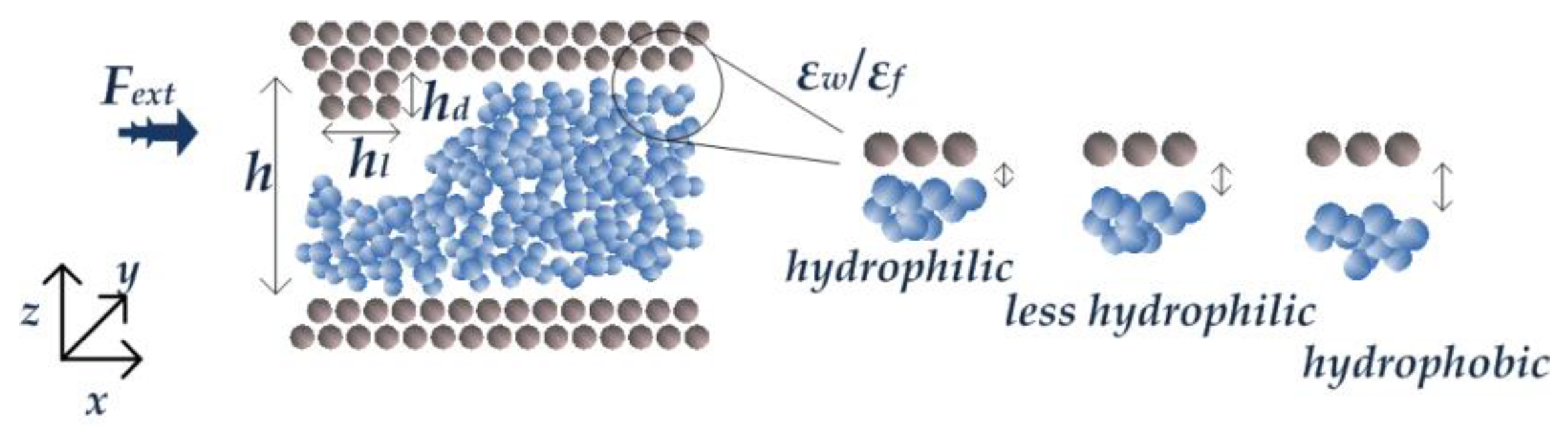
2.1. System Model
2.2. Machine Learning
2.3. Dataset Creation
2.4. Data Preprocessing
3. Results
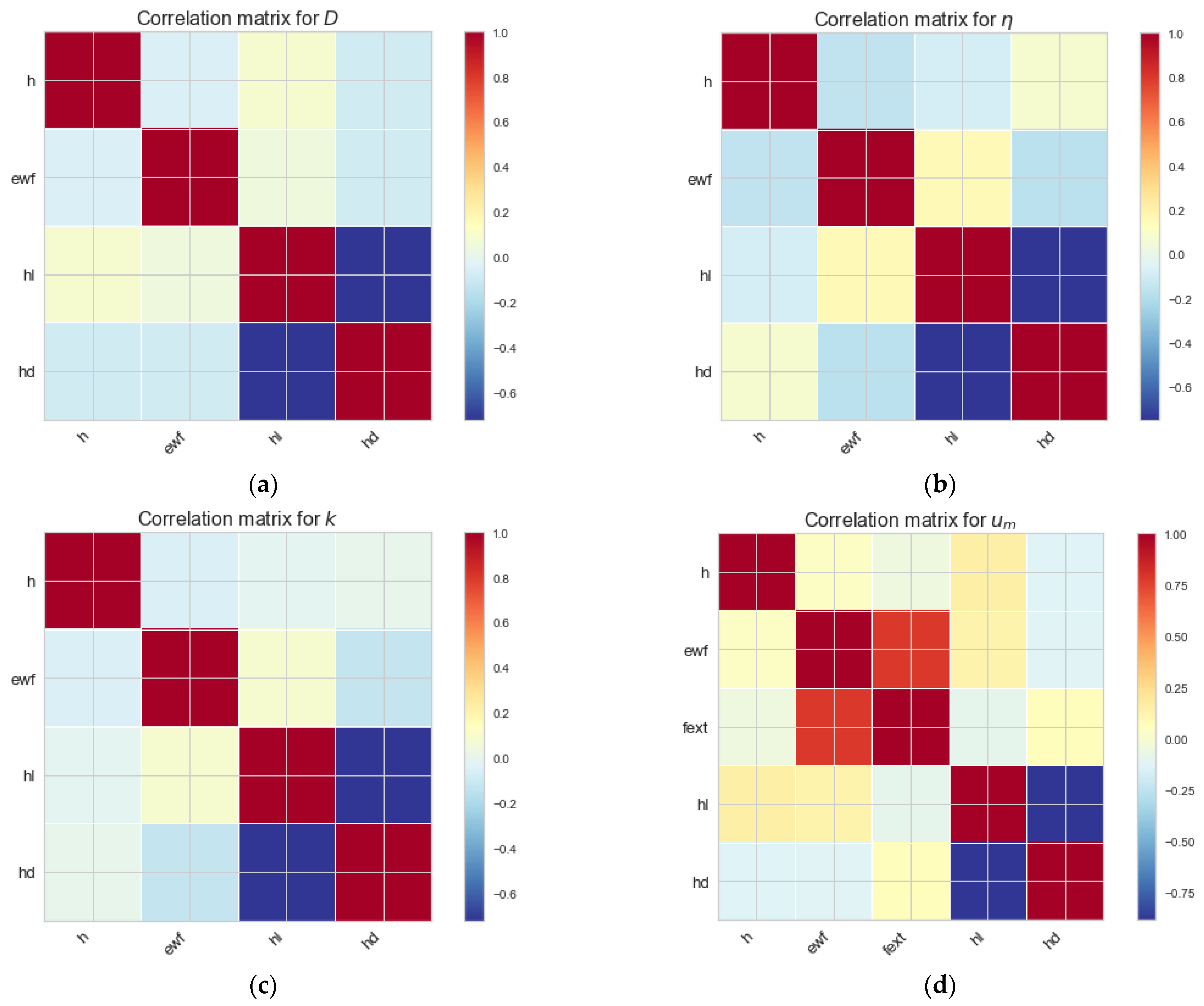
3.1. Correlations
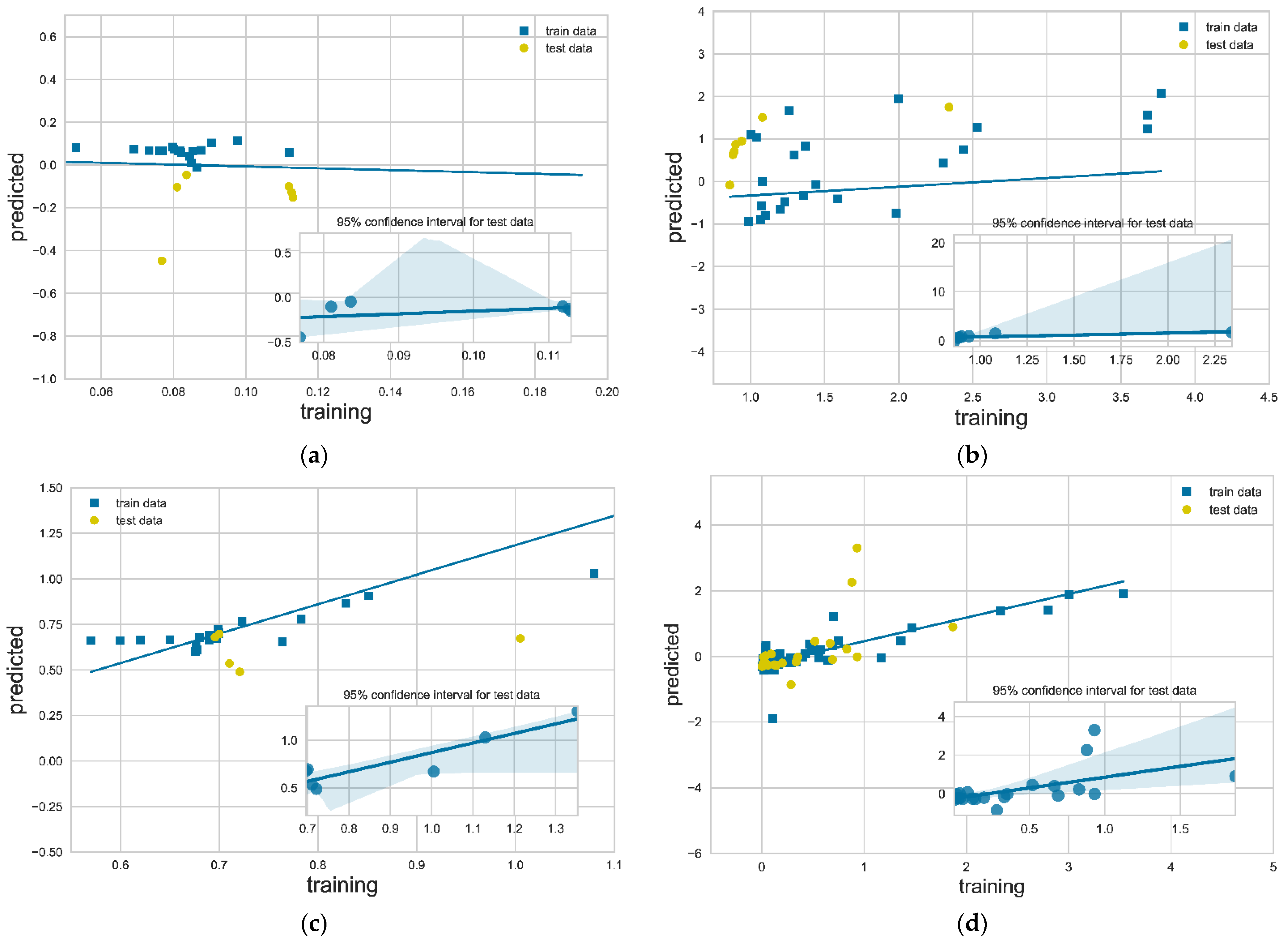
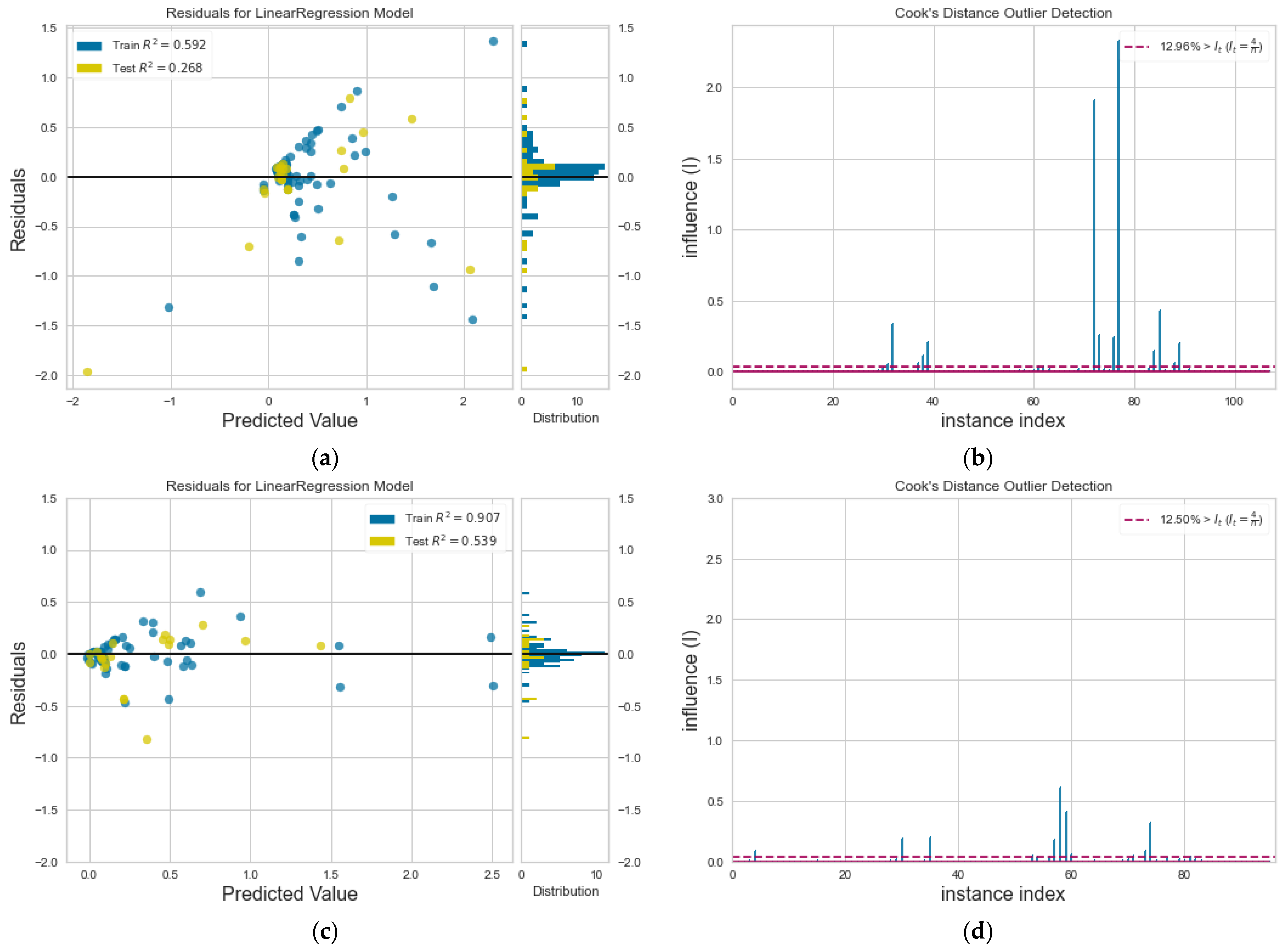
3.2. Model Accuracy
4. Discussion
5. Conclusions
Author Contributions
Funding
Institutional Review Board Statement
Informed Consent Statement
Data Availability Statement
Conflicts of Interest
Appendix A
References
- Bohn, P.W. Science and technology of electrochemistry at nano-interfaces: Concluding remarks. Faraday Discuss. 2018, 210, 481–493. [Google Scholar] [CrossRef]
- Heerema, S.J.; Dekker, C. Graphene nanodevices for DNA sequencing. Nat. Nanotech. 2016, 11, 127–136. [Google Scholar] [CrossRef] [PubMed] [Green Version]
- Karnik, R.; Castelino, K.; Fan, R.; Yang, P.; Majumdar, A. Effects of Biological Reactions and Modifications on Conductance of Nanofluidic Channels. Nano Lett. 2005, 5, 1638–1642. [Google Scholar] [CrossRef]
- Prakash, S.; Piruska, A.; Gatimu, E.N.; Bohn, P.W.; Sweedler, J.V.; Shannon, M.A. Nanofluidics: Systems and Applications. IEEE Sens. J. 2008, 8, 441–450. [Google Scholar] [CrossRef]
- Prakash, S.; Shannon, M.A.; Bellman, K. Water desalination: Emerging and existing technologies. In Aqua Nanotechnology; Reisner, D.E., Pradeep, T., Eds.; CRC Press: Boca Raton, FL, USA, 2014; pp. 533–562. [Google Scholar]
- Qiao, R.; Aluru, N.R. Atomistic simulation of KCl transport in charged silicon nanochannels: Interfacial effects. Colloids Surf. Physicochem. Eng. Asp. 2005, 267, 103–109. [Google Scholar] [CrossRef]
- Sofos, F.; Karakasidis, T.E.; Liakopoulos, A. Transport properties of liquid argon in krypton nanochannels: Anisotropy and non-homogeneity introduced by the solid walls. Int. J. Heat Mass Transf. 2009, 52, 735–743. [Google Scholar] [CrossRef]
- Sofos, F.; Karakasidis, T.E.; Liakopoulos, A. How wall properties control diffusion in grooved nanochannels: A molecular dynamics study. Heat Mass Transf. 2013, 49, 1081–1088. [Google Scholar] [CrossRef]
- Sofos, F.; Karakasidis, T.E.; Giannakopoulos, A.E.; Liakopoulos, A. Molecular dynamics simulation on flows in nano-ribbed and nano-grooved channels. Heat Mass Transf. 2016, 52, 153–162. [Google Scholar] [CrossRef]
- Lee, J.; Laoui, T.; Karnik, R. Nanofluidic transport governed by the liquid/vapour interface. Nat. Nanotechnol. 2014, 9, 317–323. [Google Scholar] [CrossRef]
- Priezjev, N.V. Effect of surface roughness on rate-dependent slip in simple fluids. J. Chem. Phys. 2007, 127, 144708. [Google Scholar] [CrossRef] [PubMed] [Green Version]
- Polster, J.W.; Acar, E.T.; Aydin, F.; Zhan, C.; Pham, T.A.; Siwy, Z.S. Gating of hydrophobic nanopores with large anions. ACS Nano 2020, 14, 4306–4315. [Google Scholar] [CrossRef]
- Bhadauria, R.; Aluru, N.R. A quasi-continuum hydrodynamic model for slit shaped nanochannel flow. J. Chem. Phys. 2013, 139, 074109. [Google Scholar] [CrossRef] [PubMed] [Green Version]
- Eral, H.B.; van den Ende, D.; Mugele, F.; Duits, M.H.G. Influence of confinement by smooth and rough walls on particle dynamics in dense hard-sphere suspensions. Phys. Rev. E 2009, 80, 061403. [Google Scholar] [CrossRef] [Green Version]
- Thompson, P.; Troian, S. A general boundary condition for liquid flow at solid surfaces. Nature 1997, 389, 360–362. [Google Scholar] [CrossRef]
- Raissi, M.; Perdikaris, P.; Karniadakis, G.E. Physics-informed neural networks: A deep learning framework for solving forward and inverse problems involving nonlinear partial differential equations. J. Comput. Phys. 2019, 378, 686–707. [Google Scholar] [CrossRef]
- Behler, J. Perspective: Machine learning potentials for atomistic simulations. J. Chem. Phys. 2016, 145, 170901. [Google Scholar] [CrossRef] [Green Version]
- Botu, V.; Ramprasad, R. Adaptive machine learning framework to accelerate ab initio molecular dynamics. Int. J. Quantum Chem. 2015, 115, 1074–1083. [Google Scholar] [CrossRef]
- Chan, H.; Narayanan, B.; Cherukara, M.J.; Sen, F.G.; Sasikumar, K.; Gray, S.K.; Chan, M.K.Y.; Sankaranarayanan, S.K.R.S. Machine Learning classical interatomic potentials for Molecular Dynamics from first-principles training data. J. Phys. Chem. C 2019, 123, 6941–6957. [Google Scholar] [CrossRef]
- Scherer, C.; Scheid, R.; Andrienko, D.; Bereau, T. Kernel-Based Machine Learning for Efficient Simulations of Molecular Liquids. J. Chem. Theory Comput. 2020, 16, 3194–3204. [Google Scholar] [CrossRef]
- Kadupitiya, J.C.S.; Sun, F.; Fox, G.; Jadhao, V. Machine learning surrogates for molecular dynamics simulations of soft materials. J. Comput. Sci. 2020, 42, 101107. [Google Scholar] [CrossRef]
- Craven, G.T.; Lubbers, N.; Barros, K.; Tretiak, S. Machine learning approaches for structural and thermodynamic properties of a Lennard-Jones fluid. J. Chem. Phys. 2020, 153, 104502. [Google Scholar] [CrossRef]
- Allers, J.P.; Harvey, J.A.; Garzon, F.H.; Alam, T.M. Machine learning prediction of self-diffusion in Lennard-Jones fluids. J. Chem. Phys. 2020, 153, 034102. [Google Scholar] [CrossRef]
- Raissi, M.; Perdikaris, P.; Karniadakis, G.E. Machine learning of linear differential equations using Gaussian processes. J. Comput. Phys. 2017, 348, 683–693. [Google Scholar] [CrossRef] [Green Version]
- Stephan, S.; Thol, M.; Vrabec, J.; Hasse, H. Thermophysical properties of the Lennard-Jones Fluid: Database and data assessment. J. Chem. Inf. Model. 2019, 59, 4248–4265. [Google Scholar] [CrossRef]
- Sofos, F.; Karakasidis, T.E.; Liakopoulos, A. Surface wettability effects on flow in rough wall nanochannels. Microfluid. Nanofluidics 2012, 12, 25–31. [Google Scholar] [CrossRef]
- Giannakopoulos, A.E.; Sofos, F.; Karakasidis, T.E.; Liakopoulos, A. A quasi-continuum multi-scale theory for self-diffusion and fluid ordering in nanochannel flows. Microfluid. Nanofluidics 2014, 17, 1011–1023. [Google Scholar] [CrossRef]
- Alpaydin, E. Machine Learning: The New AI; MIT Press: Cambridge, MA, USA, 2016. [Google Scholar]
- Pedregosa, F.; Varoquaux, G.; Gramfort, A.; Michel, V.; Thirion, B.; Grisel, O.; Blondel, M.; Prettenhofer, P.; Weiss, R.; Dubourg, V.; et al. Scikit-learn: Machine Learning in Python. JMLR 2011, 12, 2825–2830. [Google Scholar]
- Asproulis, N.; Drikakis, D. Boundary slip dependency on surface stiffness. Phys. Rev. E 2010, 81, 061503. [Google Scholar] [CrossRef] [Green Version]
- Vinogradova, O.; Belyaev, A. Wetting, roughness and hydrodynamic slip. In Nanoscale Liquid Interfaces: Wetting, Patterning and Force Microscopy at the Molecular Scale; Ondarcucu, T., Aime, J.-P., Eds.; Pan Stanford Publishing: Singapore, 2013; pp. 29–82. [Google Scholar]
- Hu, Y.Z.; Wang, H.; Guo, Y. Molecular dynamics simulation of poiseuille flow in ultra-thin film. Tribotest 1995, 1, 301–310. [Google Scholar] [CrossRef]
- Hyżorek, K.; Tretiakov, K.V. Thermal conductivity of liquid argon in nanochannels from molecular dynamics simulations. J. Chem. Phys. 2016, 144, 194507. [Google Scholar] [CrossRef] [PubMed]
- Jabbarzadeh, A.; Atkinson, J.D.; Tarner, R.I. Effect of the wall roughness on slip and rheological properties of hexadecane in molecular dynamics simulation of Couette shear flow between two sinusoidal walls. Phys. Rev. E 2000, 61, 690–699. [Google Scholar] [CrossRef]
- Markesteijn, A.P.; Hartkamp, R.; Luding, S.; Westerweel, J. A comparison of the value of viscosity for several water models using Poiseuille flow in a nano-channel. J. Chem. Phys. 2012, 136, 134104. [Google Scholar] [CrossRef] [PubMed] [Green Version]
- Sofos, F.; Karakasidis, T.E.; Liakopoulos, A. Effects of wall roughness on flow in nanochannels. Phys. Rev. E 2009, 79, 026305. [Google Scholar] [CrossRef] [PubMed]
- Sofos, F.; Karakasidis, T.E.; Liakopoulos, A. Non-Equilibrium Molecular Dynamics investigation of parameters affecting planar nanochannel flows. Contemp. Eng. Sci. 2009, 2, 283–298. [Google Scholar]
- Sofos, F.; Karakasidis, T.E.; Liakopoulos, A. Fluid structure and system dynamics in nanodevices for water desalination. Desalination Water Treat. 2015, 57, 11561–11571. [Google Scholar] [CrossRef]
- Somers, S.A.; Davis, H.T. Microscopic dynamics of fluids confined between smooth and atomically structured solid surfaces. J. Chem. Phys. 1991, 96, 5389–5407. [Google Scholar] [CrossRef]
- Toghraie Semiromi, D.; Azimian, A.R. Nanoscale Poiseuille flow and effects of modified Lennard–Jones potential function. Heat Mass Transf. 2010, 46, 791–801. [Google Scholar] [CrossRef]
- Travis, K.; Todd, B.D.; Evans, D. Departure from Navier-Stokes hydrodynamics in confined liquids. Phys. Rev. E 1997, 55, 4288–4295. [Google Scholar] [CrossRef]
- Yang, S.C. Effects of surface roughness and interface wettability on nanoscale flow in a nanochannel. Microfluid. Nanofluidics 2006, 2, 501–511. [Google Scholar] [CrossRef]
- Swamynathan, M. Mastering Machine Learning with Python in Six Steps; Apress: New York, NY, USA, 2017. [Google Scholar]
- Osborne, J.W.; Overbay, A. The power of outliers (and why researchers should ALWAYS check for them). Pract. Assess. Res. Eval. 2004, 9, 6. [Google Scholar]
- Cook, R.D. Detection of influential observation in linear regression. Technometrics 1977, 19, 15–18. [Google Scholar]
- Bengfort, B.; Bilbro, R. Yellowbrick: Visualizing the Scikit-Learn Model Selection Process. J. Open Source Softw. 2019, 4, 1075. [Google Scholar] [CrossRef]
- Fourches, D.; Muratov, E.; Tropsha, A. Trust, but verify: On the importance of chemical structure curation in cheminformatics and QSAR modeling research. J. Chem. Inf. Model. 2010, 50, 1189–1204. [Google Scholar] [CrossRef]
- Elton, D.C.; Boukouvalas, Z.; Butrico, M.S.; Fuge, M.D.; Chung, P.W. Applying machine learning techniques to predict the properties of energetic materials. Sci. Rep. 2018, 8, 9059. [Google Scholar] [CrossRef]
- Wang, A.Y.-T.; Murdock, R.J.; Kauwe, S.K.; Oliynyk, A.O.; Gurlo, A.; Brgoch, J.; Persson, K.A.; Sparks, T.D. Machine Learning for Materials Scientists: An Introductory guide toward best practices. Chem. Mater. 2020, 32, 4954–4965. [Google Scholar] [CrossRef]
- Hess, B. Determining the shear viscosity of model liquids from molecular dynamics simulations. J. Chem. Phys. 2002, 116, 209–217. [Google Scholar] [CrossRef]
- Hartkamp, R.; Ghosh, A.; Weinhart, T.; Luding, S. A study of the anisotropy of stress in a fluid confined in a nanochannel. J. Chem. Phys. 2012, 137, 044711. [Google Scholar] [CrossRef]
- Frank, M.; Drikakis, D. Thermodynamics at solid-liquid interfaces. Entropy 2018, 20, 362. [Google Scholar] [CrossRef] [Green Version]
- Cao, B.; Adutwum, L.A.; Oliynyk, A.O.; Luber, E.J.; Olsen, B.C.; Mar, A.; Buriak, J.M. How to optimize materials and devices via design of experiments and machine learning: Demonstration using organic photovoltaics. ACS Nano 2018, 12, 7434–7444. [Google Scholar] [CrossRef] [Green Version]


| Reference | D | η | k | um | |
|---|---|---|---|---|---|
| Hu et al. [32] | 10 | 2 | |||
| Hyżorek and Tretiakov [33] | 6 | ||||
| Jabarzadeh et al. [34] | 8 | ||||
| Markesteijn et al. [35] | 5 | ||||
| Sofos et al. [7,8,9,26,36,37,38] | 27 | 24 | 23 | 65 | |
| Sommers and Davies [39] | 3 | ||||
| Toghraie Semiromi and Azimian [40] | 6 | ||||
| Travis et al. [41] | 5 | ||||
| Yang [42] | 14 | ||||
| Total Points | 30 | 42 | 29 | 103 | 204 |
| () | () | ||||
|---|---|---|---|---|---|
| Values | 2.64–100.44 | 0.083–1.0 | 0.0–0.36 | 0.1–5.0 | 0.001–3.53 |
| D | 2.13 | 2.83 | 3.55 | 1.21 | - |
| η | 1.98 | 2.95 | 3.85 | 1.17 | - |
| k | 2.08 | 3.06 | 3.60 | 1.24 | - |
| 2.26 | 2.31 | 1.17 | 3.25 | 3.21 |
| Property | RMSE | MAE | R2 | wh | wewf | whl | whd | wfext |
|---|---|---|---|---|---|---|---|---|
| D | 0.023 | 0.018 | 0.790 | 0.0016 | 0.0073 | 0.0334 | 0.1270 | - |
| η | 4.732 | 3.764 | 0.380 | 0.1921 | 0.3513 | 0.2353 | 1.1005 | - |
| k | 0.231 | 0.162 | 0.998 | 0.0023 | 0.1062 | 0.4997 | 4.3263 | - |
| 0.768 | 0.549 | 0.483 | 0.0652 | −0.0499 | −0.2118 | −0.0696 | 0.8585 |
Publisher’s Note: MDPI stays neutral with regard to jurisdictional claims in published maps and institutional affiliations. |
© 2021 by the authors. Licensee MDPI, Basel, Switzerland. This article is an open access article distributed under the terms and conditions of the Creative Commons Attribution (CC BY) license (http://creativecommons.org/licenses/by/4.0/).
Share and Cite
Sofos, F.; Karakasidis, T.E. Machine Learning Techniques for Fluid Flows at the Nanoscale. Fluids 2021, 6, 96. https://doi.org/10.3390/fluids6030096
Sofos F, Karakasidis TE. Machine Learning Techniques for Fluid Flows at the Nanoscale. Fluids. 2021; 6(3):96. https://doi.org/10.3390/fluids6030096
Chicago/Turabian StyleSofos, Filippos, and Theodoros E. Karakasidis. 2021. "Machine Learning Techniques for Fluid Flows at the Nanoscale" Fluids 6, no. 3: 96. https://doi.org/10.3390/fluids6030096