Article

Turbulent Premixed Flame Modeling Using the Algebraic Flame Surface Wrinkling Model: A Comparative Study between OpenFOAM and Ansys Fluent

Department of Civil, Chemical and Environmental Engineering (DICCA), University of Genoa, 16145 Genoa, Italy
*
Authors to whom correspondence should be addressed.
Fluids 2021, 6(12), 462; https://doi.org/10.3390/fluids6120462
Submission received: 9 November 2021 / Revised: 29 November 2021 / Accepted: 29 November 2021 / Published: 17 December 2021

Abstract

:
Hereafter, we used the Algebraic Flame Surface Wrinkling (AFSW) model to conduct numerical simulations of the Paul Scherrer Institute (PSI) high-pressure, turbulent premixed Bunsen flame experiments. We implemented the AFSW model in OpenFOAM and in Ansys Fluent, and we compared the outcome of both solvers against the experimental results. We also highlight the differences between both solvers. All the simulations were performed using a two-dimensional axisymmetric model with the standard k ϵ turbulence model with wall functions. Two different fuel/air mixtures were studied, namely, a 100% C H 4 volumetric ratio and a 60% C H 4 + 40% H 2 volumetric ratio. The thermophysical and transport properties of the mixture were calculated as a function of temperature using the library Cantera (open-source suite of tools for problems involving chemical kinetics, thermodynamics, and transport processes), together with the GRI-Mech 3.0 chemical mechanism. It was found that the outcome of the AFSW model implemented in both solvers was in good agreement with the experimental results, quantitatively and qualitatively speaking. Further assessment of the results showed that, as much as the chemistry, the turbulence model and turbulent boundary/initial conditions significantly impact the flame shape and height.

1. Introduction

The study of premixed turbulent combustion is an area of active research as mastering this technology can directly translate into increased efficiency and reduced NOx and other pollutant emissions. However, modeling premixed combustion phenomena is a non-trivial task because of the interaction between turbulence and chemical reactions. To overcome this challenge, many combustion models have been developed and tested, to name a few, the eddy breakup model [1], turbulent flame speed closure [2], the eddy dissipation concept [3], the coherent flamelet model [4], the extended coherent flamelet model [5], the level set approach for corrugated flamelet regimes (G-equation models) [6,7], and the algebraic flame surface wrinkling model [8].
In this study, we performed numerical simulations of the PSI’s high-pressure, turbulent premixed Bunsen C H 4 / H 2 /air flame experiments [9,10]. The combustion process was modeled using the Algebraic Flame Surface Wrinkling (AFSW) model [8,11]. The AFSW model is an algebraic model originally derived by Muppala et al. [8] through curve fitting of the Kobayashi experiments on turbulent flame speed measurements for methane and propane flames [12]. The model was further improved by Dinkelacker et al. [11], where the authors included an effective Lewis number term to extend its applicability to blended hydrogen mixtures. This model has been validated for Bunsen-like flames and sudden expansion dump combustors [11,13,14], where good agreement has been obtained in terms of flame lengths and speeds.
Hereafter, we aimed at reproducing the results of Dinkelacker et al. [11] by using the open-source numerical library OpenFOAM [15,16] and the commercial CFD solver Ansys Fluent [17]. As this AFSW model is not readily available in OpenFOAM or Ansys Fluent, we implemented the AFSW model in both CFD solvers. In OpenFOAM, the AFSW model was implemented by modifying the solver XiFoam. In Ansys Fluent, the model was implemented using User-Defined Function (UDF). We then compared the outcome of both solvers against the experimental results. All the simulations were performed using a two-dimensional axisymmetric model with the standard k ϵ RANS turbulence model with wall functions [18,19].
The remainder of the manuscript is organized as follows. In Section 2, we review the theoretical background of premixed combustion modeling, energy equation treatment, and the calculation of the thermophysical and transport properties. In Section 3, we address the implementation details of the AFSW model in OpenFOAM. The experimental setup is briefly addressed in Section 4, and in Section 5, we cover the numerical background. Section 6 is dedicated to the discussion of the results. Finally, in Section 7, we outline the conclusions and perspectives.

2. Theoretical Background

2.1. Premixed Combustion Model

Under the assumption of simple one-step chemistry with the unity Lewis number and adiabatic conditions, the species transport equations can be reduced to a single combustion progress variable equation, as follows [2,20,21],
ρ ¯ c ˜ t + ρ ¯ u ˜ i c ˜ x i = x i ρ ¯ α + μ t S c t c ˜ x i + ω ˙ ¯ c .
In Equation (1), the transported quantity c refers to the normalized mass fraction of the products [2], which we call the progress variable. The combustion progress variable describes the thermochemical state of the mixture at any point in space and time (products and reactants). A detailed derivation of Equation (1) can be found in references [7,20,21,22,23].
The solution of Equation (1), together with additional closure models (turbulence, reaction rate source term, and turbulent flame speed) and the thermophysical and transported properties of the unburnt/burnt mixture and flame, gives the propagation of the premixed flame.
To conduct the numerical simulations, we used the CFD solvers OpenFOAM and Ansys Fluent. It is worth mentioning that Ansys Fluent [17] solves Equation (1). The CFD solver OpenFOAM [15,16], instead of solving for the progress variable c, solves for the regress variable b [24], where,
b = 1 c .
Henceforth, Equation (1) can be written in terms of the regress variable b as follows,
ρ ¯ b ˜ t + ρ ¯ u ˜ i b ˜ x i = x i ρ ¯ α + μ t S c t b ˜ x i ω ˙ ¯ b .
In Equations (1) and (3), the overbar ¯ and the tilde ˜ refer to the Reynolds and Favre averaging, respectively. In these equations, the molecular thermal diffusivity α is usually much smaller than the turbulent diffusivity μ t / S c t and can simply be neglected in RANS/URANS [20]. Recall that the molecular thermal diffusivity α is computed using the following relation,
α = λ ρ C p ,
In Equation (1) (the equation used in Ansys Fluent), the progress variable c is bounded between zero and one, where c = 0 represents the reactants (unburned state) and c = 1 represents the products (burned state). Any intermediate values between 0 < c < 1 denote the gas mixture with temperatures and composition between those of the reactants and products.
In the equation governing the regress variable b (Equation (3)), b is also bounded between zero and one. However, in this case, b = 0 represents the products and b = 1 represents the reactants. Equation (
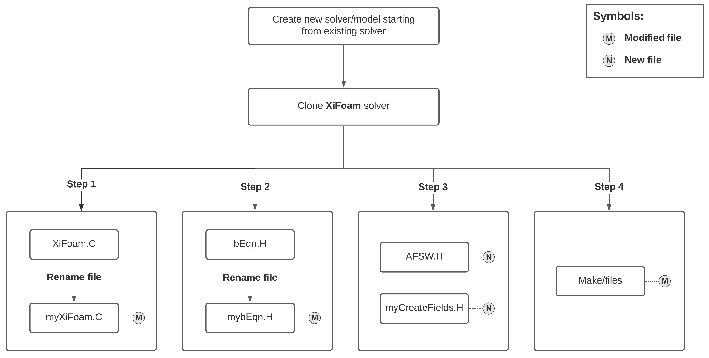
3) is the equation used in OpenFOAM and, in particular, in the solver XiFoam. OpenFOAM’s XiFoam solver is a transient solver for compressible premixed and partially premixed combustion with turbulence modeling. XiFoam is the specific OpenFOAM solver that was used in this study.
In Equations (1) and (3), evaluating the mean reaction rate source term ω ˙ ¯ is the central problem in modeling premixed turbulent combustion. This term can be modeled using algebraic methods or methods based on additional transport equations. In this study, we used an algebraic model, in particular the AFSW model [8,11,13,14]. By using this model, the reaction rate source term for the progress variable and the regress variable can be expressed as follows,
ω ˙ ¯ c = ρ u S t | c ˜ | , ω ˙ ¯ b = ρ u S t | b ˜ | ,
where the magnitude of the gradient term in Equation (5) can be evaluated as follows,
| c ˜ | i = 1 3 c ˜ x i 2 1 / 2 , | b ˜ | i = 1 3 b ˜ x i 2 1 / 2 .
The turbulent flame speed S t appearing in Equation (5) is then modeled using the AFSW model [8,11,13,14], as follows,
S t = S L 0 + S L 0 0.46 L e e f f R e t 0.25 u S L 0 0.3 P 1 atm 0.2 ,
In this equation, S L 0 is the laminar unstrained flame speed (flame without strain or stretch) and is dependent on the chemistry. It can be calculated using one-dimensional chemical kinetics solvers with detailed chemistry. In order to have a closed-form of Equation (7), the following closure relationships are used,
1 L e e f f = D α = X C H 4 D C H 4 α + X H 2 D H 2 α = X C H 4 L e C H 4 + X H 2 L e H 2 ,
R e t = u l t ν ,
l t = 0 . 09 3 / 4 k 3 / 2 ϵ ,
u = 2 3 k .
The effective Lewis number L e e f f appearing in Equation (8) models the preferential diffusion effect of the species H 2 in the unburnt mixture on the turbulent flame speed (Equation (7)) [11]. In Equation (8), the mixture molecular thermal diffusivity α is computed using Equation (4), where α is computed at the temperature at which the maximum heat is released ( T m h r r in Table 1).
In this study, we assumed the turbulent Lewis number L e t to be equal to one. This implies that the turbulent Schmidt number S c t and the turbulent Prandtl number P r t are the same. The main consequence of this assumption is that the eddy mass diffusivity and eddy thermal diffusivity are the same. In turbulent combustion modeling, this hypothesis is widely used and often necessary when conducting RANS/URANS simulations [20,22,23]. For completeness, recall that the L e t , the S c t , and the P r t numbers are defined as follows,
L e t = S c t P r t , S c t = ν t D t , P r t = ν t α t ,
by combining these expressions, we can derive a relation for the turbulent diffusivity D t (Equation (13)), where the turbulent Schmidt number S c t is assumed to be constant.
D t = ν t S c t .
It is worth noting that the evaluation of D t is not simple. The closure given in Equation (14) is often used together with the k ϵ turbulence model, where μ t is computed from the transported turbulent quantities k and ϵ . However, while it is commonly accepted that the value of the coefficient C μ is equal to 0.09, different authors have reported different values of S c t . In this study, we assumed S c t = P r t = 0.7 [22,25].
D t = C μ S c t k 2 ¯ ϵ ¯
Finally, by substituting Equation (13) into Equations (1) and (3) and by neglecting the molecular thermal diffusivity α , we obtain the following solvable equations for the progress variable c and the regress variable b,
ρ ¯ c ˜ t + ρ ¯ u ˜ i c ˜ x i = x i ρ ¯ D t c ˜ x i + ω ˙ ¯ c .
( ρ ¯ b ˜ ) t + ( ρ ¯ u ˜ i b ˜ ) x i = x i ρ ¯ D t b ˜ x i ω ˙ ¯ b .
Equation (15) or Equation (16), together with the compressible RANS equations, the k ϵ closure turbulence model, and proper boundary conditions and initial conditions, are solved using OpenFOAM’s XiFoam solver and Ansys Fluent.

2.2. Energy Equation Treatment

In OpenFOAM’s XiFoam solver, the energy equation is treated either in terms of the absolute enthalpy h a formulation (the sensible enthalpy plus the chemical enthalpy) or in terms of the internal energy e i formulation [26]. In this study, we used the absolute enthalpy formulation in OpenFOAM, namely Equation (17). In this equation, K is the specific kinetic energy and P is the thermodynamic pressure (absolute pressure). Since h a already contains the chemical enthalpy, there is no chemical heating source in Equation (17).
( ρ ¯ h ˜ a ) t + ( ρ ¯ u ˜ i h ˜ a ) x i + ( ρ ¯ K ˜ ) t + ( ρ ¯ u ˜ i K ˜ ) x i = P ¯ t + x i μ ˜ P r + μ ˜ t P r t h ˜ a x i .
In contrast, Ansys Fluent uses the sensible enthalpy h s formulation when dealing with premixed and partially premixed combustion [17]. In the formulation used hereafter (Equation (18)), the thermodynamic pressure, the specific kinetic energy, and the viscous dissipation (or viscous heating) terms are not included (these terms are often negligible in incompressible flows). Instead, it includes the chemical enthalpy h c h e m as a source term on the RHS of Equation (18), which needs to account for the conservation of energy in the sensible enthalpy formulation [17,26].
( ρ ¯ h ˜ s ) t + ( ρ ¯ u ˜ i h ˜ s ) x i = x i μ ˜ P r + μ ˜ t P r t h ˜ s x i + h ˜ c h e m .
In Ansys Fluent, the partially premixed setup was used, but with the PDF equations disabled, which is identical to perfectly premixed combustion. Therefore, all compressibility effects were taken into account using the PDF look-up tables computed by Ansys Fluent. Finally, in Equation (18), the chemical enthalpy h c h e m is defined as,
h ˜ c h e m = ω ˙ ¯ Δ H c o Y f ,
where ω ˙ ¯ is the reaction rate source term and is defined in Equation (5), Δ H c o is the lower heating value of combustion, and Y f is the fuel mixture mass fraction.

2.3. Thermophysical and Transport Properties

The thermophysical and transport properties of the unburnt/burnt mixtures and flame were calculated as a function of the temperature using the library Cantera 2.4.0 [27]. Cantera is an open-source suite of tools for problems involving chemical kinetics, thermodynamics, and transport processes. For the 1D chemistry calculations, we used the library GRI-Mech 3.0 [28]. GRI-Mech is a database of chemical reactions and associated rate constant expressions capable of the best representation of natural gas flames and ignition. It is a compilation of 325 chemical reactions and related rate coefficient expressions and thermochemical parameters for the 53 species involved in them. Previous studies have shown that the calculated S L 0 for C H 4 / H 2 /air mixtures using this mechanism is in good agreement with experimental data [29,30].
In Table 1, we show the calculated properties. In this table, the variables α , D C H 4 , and D H 2 are calculated at the maximum heat release rate temperature ( T m h r r ). As can be seen in this table, the addition of H 2 to the mixture increases the laminar flame speed S L 0 . This is attributed to higher H 2 reactivity with respect to C H 4 [31].
In Ansys Fluent, the temperature-dependent mixture properties, namely, specific heat C p , thermal conductivity λ , and dynamic viscosity μ , are calculated using polynomial models. To compute the coefficients of the polynomials, the physical properties C p , λ , and μ are calculated across the flame at certain temperature values (equally spaced between unburnt and burnt temperature) using the FreeFlame configuration in Cantera. Then, by using polynomial fitting, the coefficients of the polynomial model are obtained. In addition, the mixture law model is used to model the composition-dependent mixture specific heat [17].
On the other hand, the solver XiFoam in OpenFOAM requires the definition of the JANAF table coefficients for C p and the definition of the coefficients of the Sutherland law for the computation of the dynamic viscosity. The thermal conductivity λ is then computed from the definition of the molecular Prandtl number P r ,
P r = C p μ λ .
The JANAF table coefficients were calculated using Equations (21)–(23) [32]. In these equations, the superscript o refers to standard state pressure conditions or P = 1 atm . In Equations (21)–(23), R is the universal gas constant and H and S refer to the standard state enthalpy and entropy, respectively, both defined at a reference temperature of T r e f = 298 K.
C p o R = a 0 + a 1 T + a 2 T 2 + a 3 T 3 + a 4 T 4 ,
H o R T r e f = a 0 + a 1 2 T r e f + a 2 3 T r e f 2 + a 3 4 T r e f 3 + a 4 5 T r e f 4 + a 5 T r e f ,
S o R = a 0 ln T r e f + a 1 T r e f + a 2 2 T r e f 2 + a 3 3 T r e f 3 + a 4 4 T r e f 4 + a 6 .
The coefficients a 0 , a 1 , a 2 , a 3 , and a 4 in Equation (21) were obtained by curve fitting at different temperature values (T). Once a 0 , . . . , a 4 have been determined, they are substituted in Equations (22) and (23) at T r e f . At this point, the coefficient a 5 appearing in Equation (22) (enthalpy jump) and the coefficient a 6 appearing in Equation (23) (entropy jump) can be computed. These coefficients were calculated for low- ( 200 K to 1000 K ) and high- ( 1000 K to 6000 K ) temperature ranges for both unburnt and burnt mixtures.
The dynamic viscosity of the mixture was computed using the Sutherland law [33], which is expressed as follows,
μ = A s T 0.5 1 + T s / T ,
where μ is the temperature-dependent mixture dynamic viscosity, A s and T s are the model coefficients, and T is the varying mixture temperature. Curve fitting was performed under varying temperatures at the operating pressure. In the cases presented in this study, the operating pressure corresponded to the experimental conditions and was equal to 5 atm [9,10,11].
In XiFoam, the coefficients C p and μ must be defined separately for the unburnt and the burnt mixtures. Additionally, the molar weights of the unburnt and the burnt mixture must be defined. A Python-based Cantera script was written to achieve this, and the required properties were calculated with the GRI-Mech 3.0 mechanism. For completeness, the script is provided in the software repository [34].
The final two parameters, stoichiometric air-to-fuel mass ratio A F R s t and equivalence ratio ϕ , can be calculated using Equations (25) and (26), respectively. In Equation (26), the sub-index f u e l refers to the fuel mixture. In this study, we simulated two cases corresponding to two different fuel mixtures. The species volumetric ratio of each fuel mixture is given in Table 2.
A F R s t = m a i r m f u e l s t ,
ϕ = m f u e l m o x i d i z e r m f u e l m o x i d i z e r s t = n f u e l n o x i d i z e r n f u e l n o x i d i z e r s t ,

3. Solver Implementation in OpenFOAM

Before giving the details of the implementation of the AFSW model in OpenFOAM, it is important to reiterate that we used OpenFOAM Version 8. Regarding Ansys Fluent, we used Version 19.R1. Hereafter, we do not give details about the implementation of the AFSW model using UDF in Ansys Fluent, as this is out of the scope of this work. The interested reader can find the UDF files in the solver repository [34].
The AFSW model was directly implemented in OpenFOAM’s XiFoam solver. In Figure 1, we depict the flowchart of the implementation of the new model. In this figure and subsequent explanations, we only address the new and modified files. To follow the description of the implementation of the AFSW model in XiFoam, it is recommended to compare the code listings shown in this section with the source code of the new solver and the original solver. The source code of the new solver can be found at the following repository [34].
The implementation of the new model in OpenFOAM starts by cloning the source code of the solver XiFoam. After cloning the source code, we can proceed to implementing the model in four steps, as illustrated in Figure 1. In Step 1, we renamed the original file XiFoam.C to myXiFoam.C. In this step, we also modified the file myXiFoam.C. The modification consisted of two steps. In the first step, we added the following include directive to myXiFoam.C (Listing 1), Fluids 06 00462 i001
The second modification in the file myXiFoam.C consisted of changing the name of the include directive bEqn.H to mybEqn.H (Listing 2), Fluids 06 00462 i002
In Step 2, we changed the name of the file bEqn.H to mybEqn.H, and then, we proceeded to modify the file mybEqn.H. This modification consisted of changing the way the turbulent flame speed flux is computed, as follows (Listing 3), Fluids 06 00462 i003
Basically, we now used the unburnt density value rho_unb computed with Cantera (this value is defined later in Step 3). In this step, we also added the following include directive to access the AFSW model implemented in the file AFSW.H (Listing 4), Fluids 06 00462 i004
In Step 3, we created two new header files, namely AFSW.H and myCreateFields.H. In the AFSW.H header file, we defined the function that implements the computation of the turbulent flame speed S t in the AFSW model. Notice the correspondence between Code Listing 5 and Equation (7), which we rewrite here for clarity.
S t = S L 0 + S L 0 0.46 L e e f f R e t 0.25 u S L 0 0.3 P 1 atm 0.2 .
Fluids 06 00462 i005
In the header file myCreateFields.H, we declared all the variables required by the AFSW model implementation. Namely, R e t (Reynolds_number in the source code), l t (L_x in the source code), u (up in the source code), L e e f f (Le in the source code), ρ u (rho_unb in the source code), μ u (mu_unb in the source code), and S L 0 (Su in the source code). Notice that R e t , l t , and u were computed using Equations (9)–(11), whereas L e e f f , ρ u , μ u , and S L 0 are constant values (computed using Cantera).
The final step (Step 4) consisted of modifying the compilation instructions. The files related to the compilation are located in the sub-directory Make. In this sub-directory, we only needed to modify the source code file named file. The modification consisted of changing the name of the input file to myXiFoam.C and the name of the output executable and its default location to $(FOAM_USER_APPBIN)/myXiFoam.
At this point, we can compile the new solver/model by using OpenFOAM’s wmake command. This command compiles the new solver, and it creates the executable myXiFoam. It is worth stressing that all the variables declared in the header file myCreateFields.H are hardwired. This means that in order to run a new simulation with a different species concentration and boundary conditions, we must update this file and recompile the solver. In the solver repository [34], the interested reader can find the header file myCreateFields.H with the physical properties for both cases listed in Table 2.
For completeness, let us explain how the reaction rate source term ω ˙ ¯ is computed in Equation (16) by means of the AFSW model. Recall that the reaction rate source term of the regress equation is equal to,
ω ˙ ¯ = ρ u S t | b ˜ | .
In the source code, the reaction rate source term corresponds to the highlighted text in Listing 6. This term is computed using the variable phiSt computed as per Listing 3. The variable phiSt represents the scalar contribution ρ u S t in the reaction rate source term. Notice that phiSt is a vector quantity, but by taking the divergence of it, we can convert it to a scalar quantity. Then, the reaction rate source term is computed using an implicit source, where the contribution of the term | b ˜ | is implicitly computed in the source term. Fluids 06 00462 i006

4. Experimental Setup and Data

The experimental data referred to in this study were taken from references [9,10,11]. In Figure 2, the Bunsen-type high-pressure generic burner used in the experimental setup is depicted. Turbulence was created using a grid placed at 50 mm upstream of the inlet in the experimental test rig. The turbulent fluctuations u and length scales l t were measured at the inlet using the Particle Image Velocimetry (PIV) method. Further information about the experimental setup can be found in references [9,10,11]. In Table 3, the operating conditions of the experiments are listed. The species volumetric ratio of the fuel mixtures used in this study is listed in Table 2.

5. Numerical Background

5.1. Computational Domain and Mesh

In Figure 3 and Figure 4, we depict the computational domain and the mesh, respectively. The domain simulated corresponds to the region with dimension quotes in Figure 2. The two-dimensional mesh was made up of 76220 hexahedral elements. The minimum cell side length of the hexahedral cells was equal to 0.25 mm. This mesh criterion was taken from reference [11], where a mesh independence study was carried out. It is worth noting that the same mesh was used in OpenFOAM and Ansys Fluent, and in both solvers, we used two-dimensional axial symmetry.

5.2. Boundary and Initial Conditions

In Table 4, we list the boundary and initial conditions defined in OpenFOAM. In Ansys Fluent, the equivalent boundary conditions are defined, namely Velocity inlet, Pressure outlet, Wall, and Axis. The initial estimates of the turbulent quantities k and ϵ were obtained using Equations (27) and (28) and the values of u and l t indicated in Table 3. A fully developed velocity profile was defined at the inlet boundary (plotted in Figure 5), which was obtained from a separate two-dimensional axisymmetric pipe flow simulation. The numerical values of the boundary and initial conditions used in OpenFOAM and Ansys Fluent can be recovered from the input files shared in the software repository [34].
k = 3 2 u 2 ,
ϵ = 0 . 09 3 / 4 k 3 / 2 l t .
In this study, we used the standard k ϵ model with wall functions [18,19]. The wall functions used in OpenFOAM are shown in Table 4, whereas standard wall functions were selected in Ansys Fluent. In all simulations, the flow was assumed to be adiabatic. That is, there is no heat or mass transfer between the computational domain and the external environment. As already mentioned, in Ansys Fluent, the partially premixed setup was used, but with the PDF equations disabled, which is identical to perfectly premixed combustion.

5.3. Numerical Setup and Discretization Schemes

The governing equations were solved using the collocated finite volume method in OpenFOAM and Ansys Fluent. As the solution takes place in collocated meshes, the Rhie–Chow interpolation method was used to prevent the pressure checkerboard instability [35]. We used the same mesh in both CFD solvers, with equivalent boundary conditions, physical properties, and models (turbulence, premixed combustion, and flame). We also tried to use similar discretization schemes in order to make a fair comparison.
OpenFOAM’s XiFoam solver is a transient solver for compressible premixed and partially premixed combustion with turbulence modeling. To conduct the numerical simulations with XiFoam, we used the least-squares cell-based method for gradient discretization. In order to prevent spurious oscillations, a multi-dimensional gradient limiter were used [36]. The diffusive terms were discretized using a second-order centered differences scheme with corrections. This corrected numerical scheme for the diffusive terms takes into account mesh non-orthogonality and mesh stretching. The convective terms appearing in the governing equations were discretized using a limited linear scheme. This scheme tends towards upwind in regions of rapidly changing gradients. In this discretization scheme, the amount of upwinding can be controlled by using a blending coefficient bounded between zero and one, where one means aggressive limiting (upwinding) and zero means pure linear scheme (very accurate, but oscillatory).
For the time discretization, we used OpenFOAM’s Crank–Nicolson formulation. This formulation uses a blending coefficient bounded between zero and one. A value of zero is equivalent to the first-order Euler scheme (stable but diffusive), and a value of one is equivalent to the pure Crank–Nicolson scheme (second-order accurate, but slightly oscillatory). By setting the blending coefficient to a value between 0.7 and 0.9, we can obtain a good compromise between stability and accuracy. The time step was chosen in such a way so that the CFL number does not exceed three. To obtain extra stability, we used explicit and implicit under-relaxation, where all the Under-Relaxation Factors (URF) were set to 0.9.
The pressure–velocity coupling was achieved by means of the iterative PISO algorithm [37] (PIMPLE method in OpenFOAM), where we used at least five corrector steps and one outer-corrector step. During the iterative marching, the number of correction steps was tweaked (increased) in order to stabilize the solution and to improve the accuracy of the results. This added extra stability and accuracy comes at a higher computational cost because we need to solve the pressure, momentum, energy, and additional transport equations (turbulence equations, regress variable equation, etc.) several times. As a side note, all the simulations were started using a stable method (first-order accuracy). As the solution progressed, we switched to a more accurate, but potentially unbounded method (second-order accuracy). In the software repository [34], the interested reader will find the input files with the discretization schemes used.
In Ansys Fluent, we used an equivalent setup to discretize the gradient, convective, and diffusive terms. However, we used a coupled formulation for the pressure–velocity coupling, together with a steady time discretization, where the iterative marching was controlled using the default URF. We want to highlight that comparing the Ansys Fluent coupled method against the OpenFOAM segregated method is not a fair exercise. For steady solvers with complicated physical models, coupled solvers are more robust and have a better convergence rate (but at the cost of a higher computational cost per iteration). The coupled approach in Ansys Fluent allowed us to test and validate the AFSW model in reasonable times without sacrificing accuracy and stability. In the software repository [34], the interested reader will find the Ansys Fluent case setup with a commented text file, where it is explained how to run the simulation.
Finally, the convergence of the solution in both solvers was judged based on the shape of the flame (the brush). As soon as a steady flame shape or brush was achieved, the simulation was stopped. This requires the computation and continuous monitoring of the average field values during the simulation.

6. Results and Discussion

Figure 6 shows the comparison of the flame shapes. The experimental flame shapes were obtained using OH* chemiluminescence imaging, as described in reference [10]. The numerical flame shapes were obtained using the scalar variable c ˜ (Favre-averaged progress variable), which was converted to the scalar variable c ¯ (Reynolds-averaged progress variable) by means of Equation (29) [20]. This approach was adopted since Reynolds averaging provides the mean value over a time sequence, similar to the averaging in the experiments, where simultaneous images are averaged to obtain the mean flame shape. In Equation (29), the sub-index u refers to unburnt conditions and the sub-index b refers to burnt conditions.
τ = ρ u ρ b 1 , c ¯ = ( 1 + τ ) c ˜ 1 + τ c ˜
From Figure 6, we can observe that the AFSW model implemented in Ansys Fluent and in OpenFOAM provided reasonable good qualitative agreement with the experimental results for both cases, namely 100 % C H 4 and 60 % C H 4 + 40 % H 2 . The model captured the flame shortening effect due to the L e e f f and S L 0 terms appearing in Equation (7). As the H 2 content increased, S L 0 increased as well (refer to Table 1). L e e f f decreased due to high mass diffusivity ( D H 2 ); consequently, S t increased.
In Figure 7, Figure 8 and Figure 9, we plot the quantitative results as a function of the c ¯ distribution along the axisymmetric axis. In particular, we plot the c ¯ distribution, the flame height, and the turbulent flame speed at c ¯ = 0.5 , respectively. A value of c ¯ = 0.5 corresponds to the mid-isosurface between the unburned state (reactants) and the burned state (products).
In Figure 8, the flame height ( h c ¯ = 0.5 ) was calculated from Figure 7, by projecting the intersection points of the line c ¯ = 0.5 (green line in Figure 7) and the numerical c ¯ distributions over the abscissa. Note that the values plotted in Figure 7 correspond to the values sampled along the axisymmetric axis (refer to Figure 3). The turbulent flame speeds ( S t , c ¯ = 0.5 ) in Figure 9 were calculated using Kobayashi’s method [8].
In reference [38], it was stated that the first term on the RHS of Equation (1) controls the flame brush thickness and the second term (which is a function of S t , c ¯ = 0.5 ) controls the flame length. Based on this statement, the good agreement of the flame brush thicknesses with the experiments confirmed the validity of the turbulent Schmidt number used in the CFD simulations ( S c t = P r t = 0.7 ).
Comparing the Ansys Fluent and OpenFOAM’s XiFoam solver’ results, Figure 6 shows that XiFoam slightly over-predicted the flame height compared to Ansys Fluent. Discrepancies in terms of flame heights can be better seen in Figure 8. For the case 100 % C H 4 , both solvers predicted shorter flames than the experiments. For the case 60 % C H 4 + 40 % H 2 , XiFoam slightly over-predicted the flame height, whereas Ansys Fluent better predicted the flame height (refer Figure 8). Comparing Figure 8 and Figure 9, it can be evidenced that h c ¯ = 0.5 and S t , c ¯ = 0.5 are inversely proportional.
As seen in Equations (1) and (3), the RHS depends on the turbulence model via the scalar variables μ t and S t . Therefore, discrepancies between Ansys Fluent and XiFoam can be attributed to the specific implementation of the turbulence model and the additional corrections implemented. On the other hand, the turbulence flame speed S t , responsible for the turbulence chemistry interaction, strongly depends on the turbulence model through the u and l t terms. Hence, the turbulence model is of paramount importance when modeling combustion.

7. Conclusions and Perspectives

In this study, we implemented the Algebraic Flame Surface Wrinkling (AFSW) model in the CFD solvers Ansys Fluent and OpenFOAM, and we compared their performance. We also outlined the main differences between both solvers. As a benchmark case, we used the Paul Scherrer Institute (PSI) high-pressure, turbulent premixed Bunsen flame experiments [10].
It was found that the outcome of the AFSW model implemented in both solvers was in good agreement with the experimental results described in [10], quantitatively and qualitatively speaking. Further assessment of the results showed that, as much as the chemistry, the turbulence model and turbulent conditions (boundary and initial conditions) significantly impacts the flame shape and height. Differences in the results obtained between both solvers can also be attributed to the way how the magnitude of the gradient is computed in Equation (5). In OpenFOAM, the term | b ˜ | is computed implicitly in the source term, whereas in Ansys Fluent, the term | c ˜ | is computed explicitly.
Regarding the pressure–velocity coupling method used in Ansys Fluent and OpenFOAM, we would like to stress that comparing the coupled method in Ansys Fluent against the segregated formulation in OpenFOAM is not an impartial exercise. It is known that for steady problems with complex physical models (e.g., turbulence, combustion, finite rate chemistry, and so on), coupled solvers perform much better than segregated solvers. The main reason for choosing the coupled solver in Ansys Fluent was driven by the convergence rate, stability, and robustness. We also noticed that the convergence rate of the segregated solvers in Ansys Fluent was negatively affected when using more difficult geometries or complex physical models, in some cases, to the point that they performed worse than in OpenFOAM. Overall, the coupled pressure–velocity coupling allowed us to obtain fast outcomes without giving up robustness, accuracy, and stability. Therefore, we were able to validate the AFSW model in reasonable times.
To further improve the results presented in this manuscript and to reduce the uncertainty related to the numerical simulations and physical models, we envisage extending the numerical simulations to three-dimensional domains (abandoning in this way the axial symmetry hypothesis), a better estimation of the turbulent conditions (boundary and initial conditions), and the inclusion of the turbulence grid upstream of the domain (as illustrated in Figure 2). To facilitate the monitoring of the solution, we also envisage the use of image similarity methods to compare in real time a target image (experimental results) with a source image (numerical results), similar to what was presented in reference [39].

Author Contributions

Conceptualization, H.K. and J.G.; methodology, H.K. and J.G.; software, H.K.; validation, H.K.; formal analysis, H.K. and J.G.; investigation, H.K. and J.G.; resources, H.K. and J.G.; data curation, J.G.; writing—original draft preparation, H.K. and J.G.; writing—review and editing, H.K. and J.G.; visualization, J.G.; supervision, J.G.; project administration, J.G.; funding acquisition, H.K. and J.G. All authors have read and agreed to the published version of the manuscript.

Funding

This work is part of the Marie Skłodowska-Curie Initial Training Network Pollution Know-how and Abatement (POLKA). The authors gratefully acknowledge the financial support from the European Commission under the call H2020-MSCA-ITN-2018.

Data Availability Statement

The data presented in this study are openly available in figshare at https://doi.org/10.6084/m9.figshare.16778914.

Acknowledgments

This work was conducted as part of the courses “Turbulence and CFD Models” and “Introduction to General CFD Using OpenFOAM Technology” held by Joel Guerrero at the University of Genoa, Italy.

Conflicts of Interest

The authors declare no conflict of interest. The funders had no role in the design of the study; in the collection, analyses, or interpretation of the data; in the writing of the manuscript; nor in the decision to publish the results.

Abbreviations

¯ Reynolds average.
˜ Favre average.
α Thermal diffusivity (molecular), measured in m 2 / s .
Δ H c o                Lower heating value of combustion, measured in J / kg .
ϵ Turbulence dissipation rate, measured in m 2 / s 3 .
λ Thermal conductivity, measured in W / m · K .
μ Dynamic viscosity, measured in kg / m · s .
Gradient operator.
ν Kinematic viscosity, m 2 / s .
ω ˙ ¯ Reaction rate source term, measured in kg / m 3 · s .
ω ˙ ¯ b ω ˙ ¯ in the regress variable b equation, measured in kg / m 3 · s .
ω ˙ ¯ c ω ˙ ¯ in the progress variable c equation, measured in kg / m 3 · s .
ϕ Equivalence ratio, non-dimensional.
ρ Density, measured in kg / m 3 .
τ Heat release factor, non-dimensional.
aJANAF table coefficient, non-dimensional.
A s Sutherland model coefficient, measured in kg / m · s · K .
A F R Air-to-fuel ratio, non-dimensional.
C p Specific heat, measured in J / kg · K .
C p o Standard state specific heat, measured in J / kg · K .
C H 4 Methane species.
DBinary mass diffusivity, measured in m 2 / s .
hEnthalpy, measured in J / kg .
H o Standard state enthalpy, measured in J / kg .
H 2 Hydrogen species.
KSpecific kinetic energy, measured in m 2 / s 2 .
l t Turbulence length scale, measured in m .
mMass, measured in kg .
nMole number, measured in mol .
N O x Nitrogen Oxide.
N 2 Nitrogen species.
O 2 Oxygen species.
RUniversal gas constant, measured in J / kg · K .
S o Standard state entropy, measured in J / kg · K .
S t Turbulent flame speed, measured in m / s .
S L 0 Unstrained adiabatic laminar flame speed, measured in m / s .
TTemperature, measured in K .
T s Sutherland model coefficient, measured in K .
T r e f Standard state temperature, measured in K .
u Turbulent fluctuating velocity, measured in m / s .
XMolar ratio, non-dimensional.
Y f Fuel mixture mass fraction, non-dimensional.
bRegress variable, non-dimensional.
cProgress variable, non-dimensional.
kTurbulent kinetic energy, measured in m 2 / s 2 .
L e Lewis number, non-dimensional.
PAbsolute pressure, measured in Pa .
P r Prandtl number, non-dimensional.
R e Reynolds number, non-dimensional.
S c Schmidt number, non-dimensional.
tTime, measured in s .
uVelocity, measured in m / s .
xSpatial coordinates, measured in m .
Sub-indices
a d Adiabatic conditions.
a i r Mix of O 2 and N 2 species.
a Absolute.
b Burnt mixture property.
c h e m Chemical.
C H 4 Methane species.
e f f Effective.
f Fuel.
f u e l 100 % C H 4 or 60 % C H 4 + 40 % H 2 .
H 2 Hydrogen species.
i Index of the spatial dimension, where i = 1 , 2 , 3 .
m h r r Property temperature at which the maximum heat is released.
o x i d i z e r O 2 species.
s t Stoichiometric condition.
s Sensible.
t Turbulent property.
u Unburnt mixture property.
Acronyms  
AFSWAlgebraic Flame Surface Wrinkling.
CFDComputational Fluid Dynamics.
JANAFJoint Army, Navy, and Air Force.
PDFProbability Density Function.
PSIPaul Scherrer Institute
RANSReynolds-Averaged Navier–Stokes.
RHSRight-Hand Side.
SIMPLESemi-Implicit Method for Pressure Linked Equations.
k ϵ Standard k ϵ turbulence model.
UDFUser-Defined Function.
URANSUnsteady Reynolds-Averaged Navier–Stokes.

References

  1. Spalding, D.B. Development of the eddy-break-up model of turbulent combustion. In Symposium (International) on Combustion; Elsevier: Amsterdam, The Netherlands, 1977; Volume 16, pp. 1657–1663. [Google Scholar] [CrossRef]
  2. Zimont, V.; Polifke, W.; Bettelini, M.; Weisenstein, W. An efficient computational model for premixed turbulent combustion at high reynolds numbers based on a turbulent flame speed closure. J. Eng. Gas Turbines Power 1998, 120, 526–532. [Google Scholar] [CrossRef]
  3. Magnussen, B.; Hjertager, B. On mathematical modeling of turbulent combustion with special emphasis on soot formation and combustion. In Symposium (International) on Combustion; Elsevier: Amsterdam, The Netherlands, 1977; Volume 16, pp. 719–729. [Google Scholar] [CrossRef]
  4. Poinsot, T.; Veynante, D.; Candel, S. Diagrams of premixed turbulent combustion based on direct simulation. In Symposium (International) on Combustion; Elsevier: Amsterdam, The Netherlands, 1991; Volume 23, pp. 613–619. [Google Scholar] [CrossRef]
  5. Colin, O.; Benkenida, A.; Angelberger, C. 3d Modeling of Mixing, Ignition and Combustion Phenomena in Highly Stratified Gasoline Engines. Oil Gas Sci. Technol.-Rev. IFP 2003, 58, 47–62. [Google Scholar] [CrossRef] [Green Version]
  6. Peters, N. A spectral closure for premixed turbulent combustion in the flamelet regime. J. Fluid Mech. 1992, 242, 611–629. [Google Scholar] [CrossRef]
  7. Peters, N. Turbulent Combustion; Cambridge University Press: Cambridge, UK, 2000. [Google Scholar] [CrossRef]
  8. Muppala, S.; Aluri, N.; Dinkelacker, F.; Leipertz, A. Development of an algebraic reaction rate closure for the numerical calculation of turbulent premixed methane, ethylene, and propane/air flames for pressures up to 1.0 MPa. Combust. Flame 2005, 140, 257–266. [Google Scholar] [CrossRef]
  9. Griebel, P.; Boschek, E.; Janson, P. Lean blowout limits and NOx emissions of turbulent, lean premixed, hydrogen-enriched methane/air flames at high pressure. J. Eng. Gas Turbines Power 2007, 129, 404–410. [Google Scholar] [CrossRef]
  10. Siewert, P. Flame Front Characteristics of Turbulent Lean Premixed Methane/Air Flames at High-Pressure. Ph.D. Thesis, Swiss Federal Institute of Technology Zurich (ETH Zurich), Zürich, Switzerland, 2006. [Google Scholar] [CrossRef]
  11. Dinkelacker, F.; Manickam, B.; Muppala, S. Modelling and simulation of lean premixed turbulent methane/hydrogen/air flames with an effective Lewis number approach. Combust. Flame 2011, 158, 1742–1749. [Google Scholar] [CrossRef]
  12. Kobayashi, H.; Tamura, T.; Maruta, K.; Niioka, T.; Williams, F. Burning velocity of turbulent premixed flames in a high-pressure environment. Proc. Combust. Inst. 1996, 26, 389–396. [Google Scholar] [CrossRef]
  13. Aluri, N.; Muppala, S.; Dinkelacker, F. Large-Eddy simulation of lean premixed turbulent flames of three different combustion configurations using a novel reaction closure. Flow Turbul. Combust. 2008, 80, 207–224. [Google Scholar] [CrossRef]
  14. Manickam, B.; Franke, J.; Muppala, S.; Dinkelacker, F. Large-eddy Simulation of Triangular-stabilized Lean Premixed Turbulent Flames: Quality and Error Assessment. Flow Turbul. Combust. 2012, 88, 1573–1987. [Google Scholar] [CrossRef]
  15. The OpenFOAM Foundation. Available online: http://www.openfoam.org (accessed on 1 December 2021).
  16. Weller, H.G.; Tabor, G.; Jasak, H.; Fureby, C. A tensorial approach to computational continuum mechanics using object-oriented techniques. Comput. Phys. 1998, 12, 620–631. [Google Scholar] [CrossRef]
  17. Ansys Fluent Academic Research, Release 19, Help System, Ansys Fluent Theory Guide; Ansys, Inc.
  18. Launder, B.; Spalding, D. The numerical computation of turbulent flows. Comput. Methods Appl. Mech. Eng. 1974, 3, 269–289. [Google Scholar] [CrossRef]
  19. Hanjalic, K. Two-Dimensional Asymmetric Turbulent Flow in Ducts. Ph.D. Thesis, Faculty of Engineering, University of London, London, UK, 1970. Available online: http://hdl.handle.net/10044/1/8036 (accessed on 1 December 2021).
  20. Poinsot, T.; Veynante, D. Theoretical and Numerical Combustion, 3rd ed.; Institut de Mécanique des Fluides de Toulouse: Toulouse, France, 2012; Available online: http://elearning.cerfacs.fr/combustion/onlinePoinsotBook/buythirdedition/index.php (accessed on 1 December 2021).
  21. Libby, P.A.; Williams, F.A. Turbulent Reacting Flows; Springer: Berlin/Heidelberg, Germany, 1980. [Google Scholar] [CrossRef]
  22. Lipatnikov, A. Fundamentals of Premixed Turbulent Combustion, 1st ed.; CRC Press: Boca Raton, FL, USA, 2012. [Google Scholar] [CrossRef]
  23. Kuo, K.K.; Acharya, R. Fundamentals of Turbulent and Multiphase Combustion, 1st ed.; Wiley: New York, NY, USA, 2012. [Google Scholar] [CrossRef]
  24. Weller, H.; Tabor, G.; Gosman, A.; Fureby, C. Application of a flame-wrinkling LES combustion model to a turbulent mixing layer. Proc. Combust. Inst. 1998, 27, 899–907. [Google Scholar] [CrossRef]
  25. Yeung, P.K. Lagrangian investigations of turbulence. Annu. Rev. Fluid Mech. 2002, 34, 115–142. [Google Scholar] [CrossRef]
  26. Iurashev, D. Numerical and Analytical Study of Combustion Instabilities in Industrial Gas Turbines. Ph.D. Thesis, University of Genoa, Genoa, Italy, 2012. [Google Scholar]
  27. Goodwin, D.G.; Speth, R.L.; Moffat, H.K.; Weber, B.W. Cantera: An Object-oriented Software Toolkit for Chemical Kinetics, Thermodynamics, and Transport Processes. Version 2.5.1. Available online: https://www.cantera.org (accessed on 1 December 2021). [CrossRef]
  28. Smith, G.P.; Golden, D.M.; Frenklach, M.; Moriarty, N.W.; Eiteneer, B.; Goldenberg, M.; Bowman, C.T.; Hanson, R.K.; Song, S.; Gardiner, W.C.; et al. GRI-Mech 3.0. Available online: http://combustion.berkeley.edu/gri-mech/version30/text30.html (accessed on 1 December 2021).
  29. Donohoe, N.; Heufer, A.; Metcalfe, W.K.; Curran, H.J.; Davis, M.L.; Mathieu, O.; Plichta, D.; Morones, A.; Petersen, E.L.; Guthe, F. Ignition delay times, laminar flame speeds, and mechanism validation for natural gas/hydrogen blends at elevated pressures. Combust. Flame 2014, 161, 1432–1443. [Google Scholar] [CrossRef] [Green Version]
  30. Ji, C.; Wang, D.; Yang, J.; Wang, S. A comprehensive study of light hydrocarbon mechanisms performance in predicting methane/hydrogen/air laminar burning velocities. Int. J. Hydrog. Energy 2017, 42, 17260–17274. [Google Scholar] [CrossRef]
  31. Kutkan, H.; Amato, A.; Campa, G.; Ghirardo, G.; Hilares, L.T.W.C.; Asoy, E. Modelling of Turbulent Premixed CH4/H2/Air Flames Including the Influence of Stretch and Heat Losses. J. Eng. Gas Turbines Power 2021. [Google Scholar] [CrossRef]
  32. Gordon, S.; McBride, B. Computer Program for Calculation of Complex Chemical Equilibrium Compositions and Applications. NASA Reference Publication 1311. 1994. Available online: https://shepherd.caltech.edu/EDL/PublicResources/sdt/refs/NASA-RP-1311-1.pdf (accessed on 1 December 2021).
  33. LII, W.S. The viscosity of gases and molecular force. Lond. Edinb. Dublin Philos. Mag. J. Sci. 1893, 36, 507–531. [Google Scholar] [CrossRef] [Green Version]
  34. Guerrero, J.; Kutkan, H. Case repository-Turbulent Premixed Flame Modeling using The Algebraic Flame Surface Wrinkling (AFSW) Model. A Comparative Study Between OpenFOAM and Ansys Fluent. figshare. Software. Available online: https://figshare.com/articles/software/Case_repository_-_Turbulent_Premixed_Flame_Modeling_using_The_Algebraic_Flame_Surface_Wrinkling_AFSW_Model_A_Comparative_Study_Between_OpenFOAM_and_Ansys_Fluent_/16778914 (accessed on 1 December 2021). [CrossRef]
  35. Rhie, C.M.; Chow, W.L. Numerical study of the turbulent flow past an airfoil with trailing edge separation. AIAA J. 1983, 21, 1525–1532. [Google Scholar] [CrossRef]
  36. Kim, S.; Makarov, B.; Caraeni, D. A Multidimensional Linear Reconstruction Scheme for Arbitrary Unstructured Grid. In Proceedings of the AIAA 16th Computational Fluid Dynamics Conference, Orlando, FL, USA, 23–26 June 2003. [Google Scholar] [CrossRef]
  37. Issa, R.I. Solution of the implicitly discretized fluid flow equations by operator-splitting. J. Comput. Phys. 1985, 62, 40–65. [Google Scholar] [CrossRef]
  38. Lipatnikov, A.; Chomiak, J. Turbulent flame speed and thickness: Phenomenology, evaluation, and application in multi-dimensional simulations. Prog. Energy Combust. Sci. 2002, 28, 1–74. [Google Scholar] [CrossRef]
  39. Guerrero, J.; Mantelli, L.; Naqvi, S.B. Cloud-Based CAD Parametrization for Design Space Exploration and Design Optimization in Numerical Simulations. Fluids 2020, 5, 36. [Google Scholar] [CrossRef] [Green Version]
Figure 1. Flowchart of the new solver/model development and implementation.
Fluids 06 00462 g001
Figure 2. Schematic view of the PSI generic, high-pressure Bunsen burner. Image taken from reference [10].
Fluids 06 00462 g002
Figure 3. Computational domain and dimensions. The figure is not to scale.
Fluids 06 00462 g003
Figure 4. Visualization of the two-dimensional mesh.
Fluids 06 00462 g004
Figure 5. Inlet velocity profile computed using a precursor simulation. The inlet extreme is located at 12.5 mm from the pipe axis line.
Fluids 06 00462 g005
Figure 6. Comparison of flame shapes (brush). Top row: experimental normalized OH* chemiluminescence [10]. Middle row: numerical flame shapes visualization using c ¯ (Ansys Fluent results). Bottom row: numerical flame shapes using c ¯ (OpenFOAM results). The left column of all rows corresponds to the case 100% C H 4 . The right column of all rows corresponds to the case 60% C H 4 + 40% H 2 .
Fluids 06 00462 g006
Figure 7. Plot of the c ¯ distribution over the axisymmetric axis. In the figure, the horizontal green line represents c ¯ = 0.5 (a value of c ¯ = 0.5 corresponds to the mid-isosurface between the unburned state and the burned state). The intersection of this line with the axial c ¯ distributions (the numerical results) was used to compute the flame height plotted in Figure 8.
Fluids 06 00462 g007
Figure 8. Comparison of the numerical and experimental flame heights estimated at c ¯ = 0.5 ( h c ¯ = 0.5 ). The flame height was calculated as shown in Figure 7.
Fluids 06 00462 g008
Figure 9. Comparison of the numerical and experimental flame speeds at c ¯ = 0.5 ( S t , c ¯ = 0.5 ). The flame speed was calculated using Kobayashi’s method [8].
Fluids 06 00462 g009
Table 1. Premixed mixture properties. In the table, the sub-index u refers to unburnt conditions. The sub-index a d refers to adiabatic conditions. The sub-index m h r r refers to the temperature at which the maximum heat is released. The sub-indices C H 4 and H 2 refer to the species. The variable ϕ is the equivalence ratio and is computed using Equation (26).
X CH 4 X H 2 ϕ T u P ρ u μ u D CH 4 D H 2 α S L 0 T mhrr T ad
( ) ( ) ( ) ( K ) ( atm ) ( kg / m 3 ) ( m 2 / s ) ( m 2 / s ) ( m 2 / s ) ( m 2 / s ) ( m / s ) ( K ) ( K )
1.00.00.567352.523.25 × 10 5 7.93 × 10 5 2.60 × 10 4 7.56 × 10 5 0.23216061777
0.60.40.567352.463.25 × 10 5 7.79 × 10 5 2.55 × 10 4 8.05 × 10 5 0.33415891803
Table 2. Species volumetric ratio of the fuel mixtures studied.
Species Volumetric Ratio
C H 4 H 2
Fuel mixture—Case 1100%0%
Fuel mixture—Case 260%40%
Table 3. Experiment conditions [9,10,11].
TP ϕ u inlet u L t
(K)(atm)(−) m / s m / s mm
67350.5406.162.2
Table 4. Boundary conditions and initialization type used in OpenFOAM. In the table, the abbreviations stand for: FV = fixedValue, C = Calculated, ZG = zeroGradient, NS = noSlip, UDP = User-Defined velocity profile (plotted in Figure 5), KWF = kqRWallFunction, EWF = epsilonWallFunction, NKWF = nutkWallFunction.
Boundary ConditionInitial Conditions
VariableInletOutletWallInitialization Type
kFVZGKWFuniform
ϵ FVZGEWFuniform
ν t CZGNKWFuniform
UUDPZGNSuniform
pZGFVZGuniform
TFVZGZGuniform
bFVZGZGuniform
Publisher’s Note: MDPI stays neutral with regard to jurisdictional claims in published maps and institutional affiliations.

