
On Determining the Critical Velocity in the Shot Sleeve of a High-Pressure Die Casting Machine Using Open Source CFD


Abstract
:1. Introduction
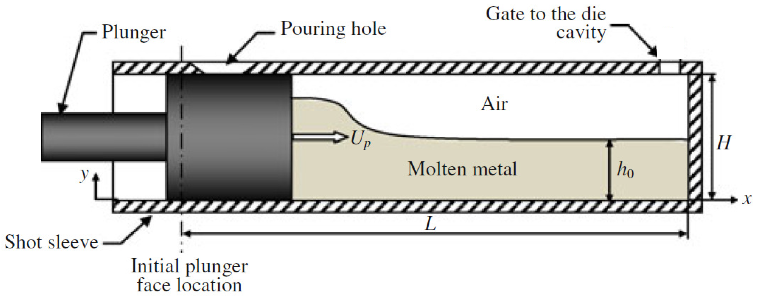
2. Theory
3. Solver Development and Testing
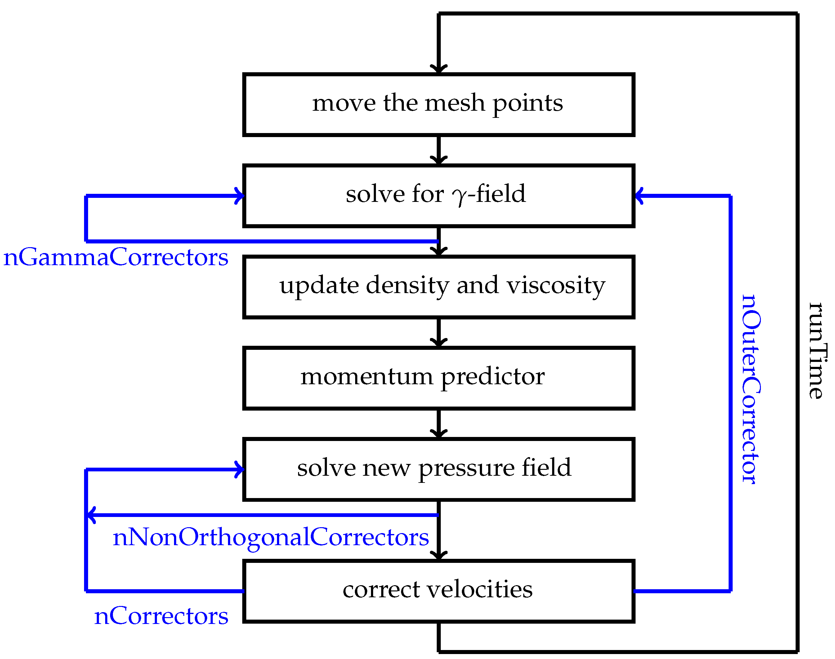
3.1. Development
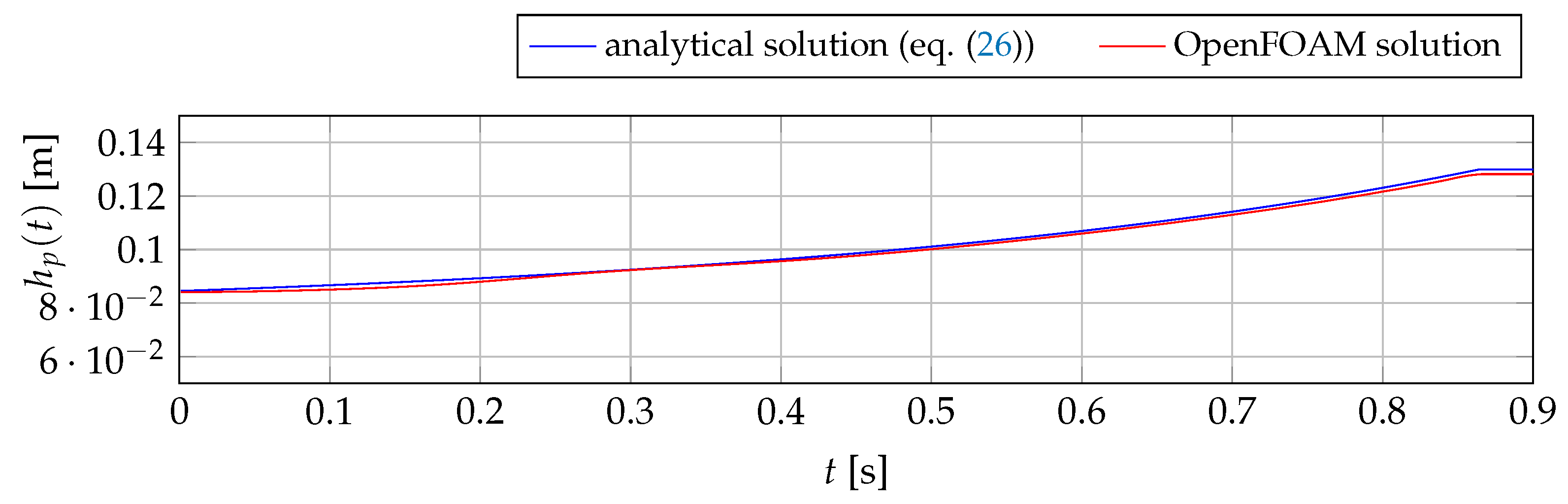
3.2. Testing
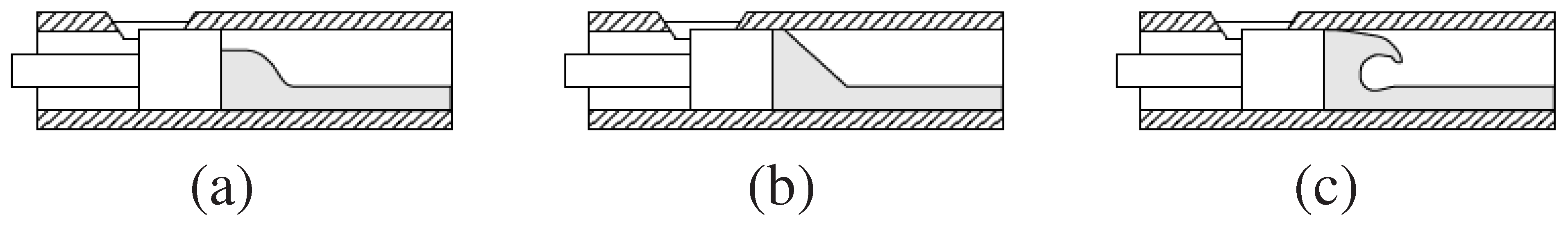
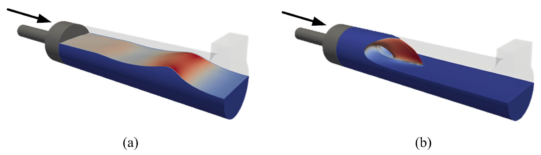
- at s, the wave first hits the wall at and reflects;
- at s, the wave at the plunger surface hits the ceiling of the chamber—from this time onwards, the plunger no longer continues to accelerate, but moves at constant speed;
- at s, the reflected wave reaches the plunger surface;
- at s (or slightly less), the melt first exits the outlet.
4. Results and Discussion
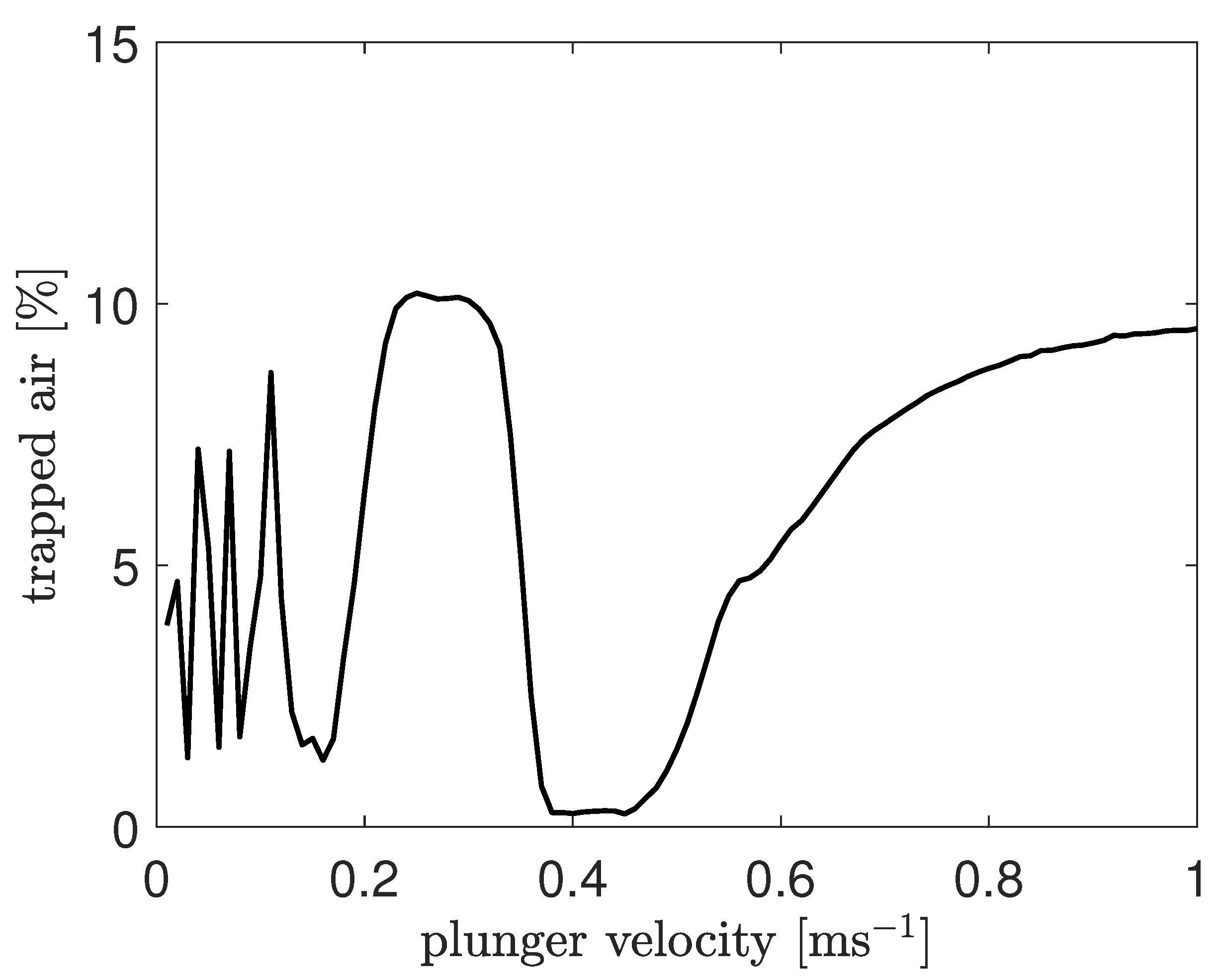
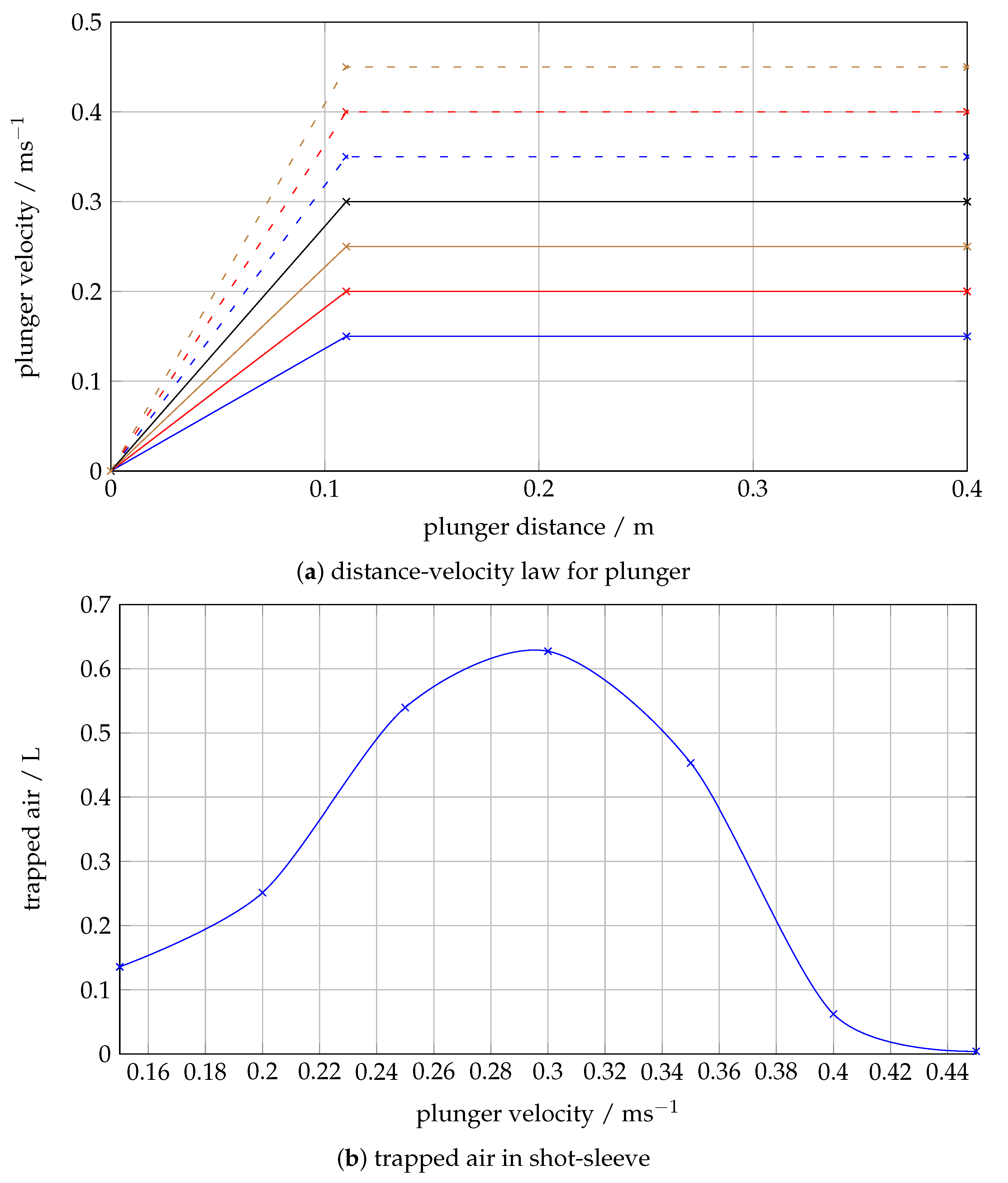
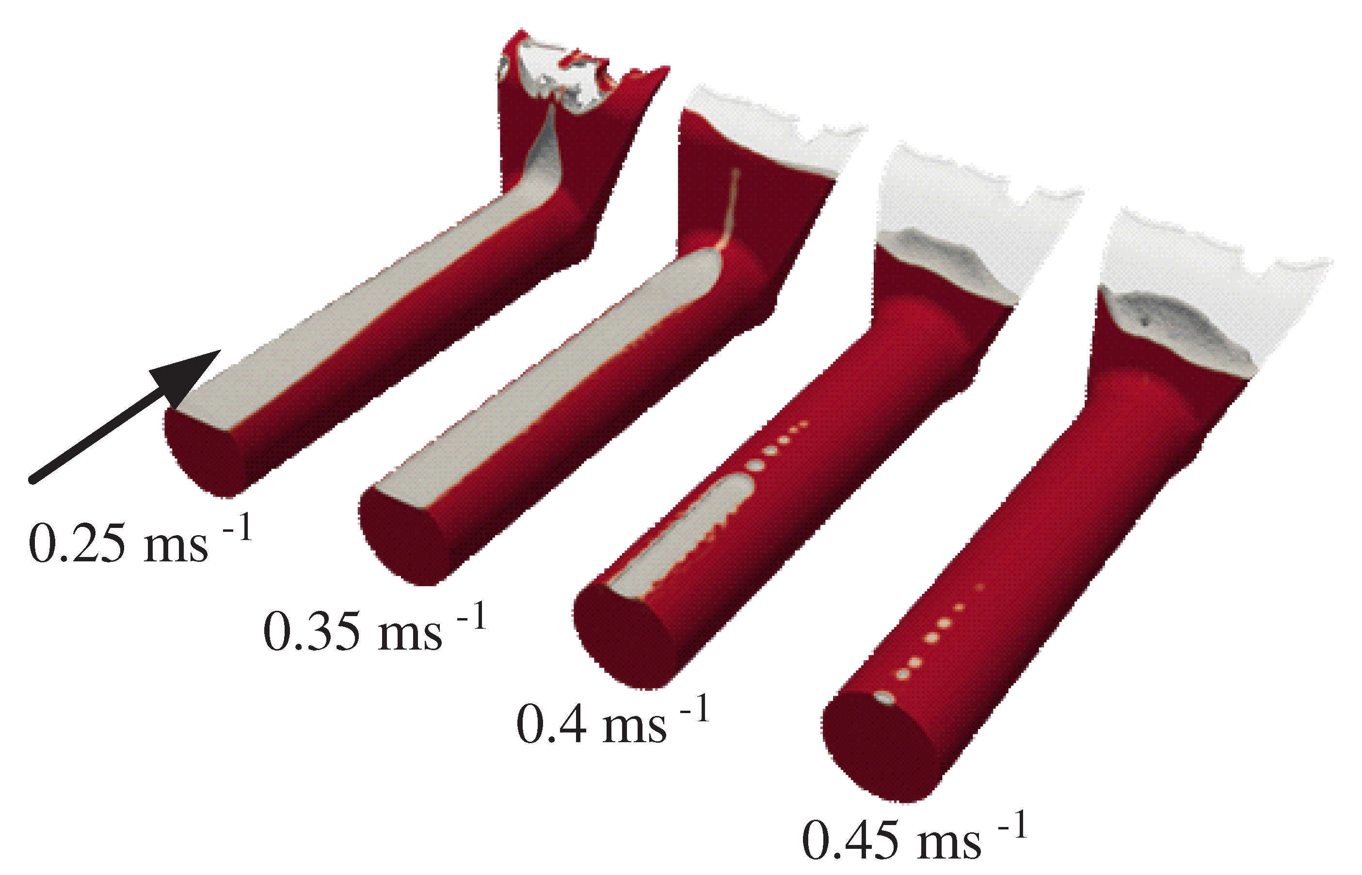
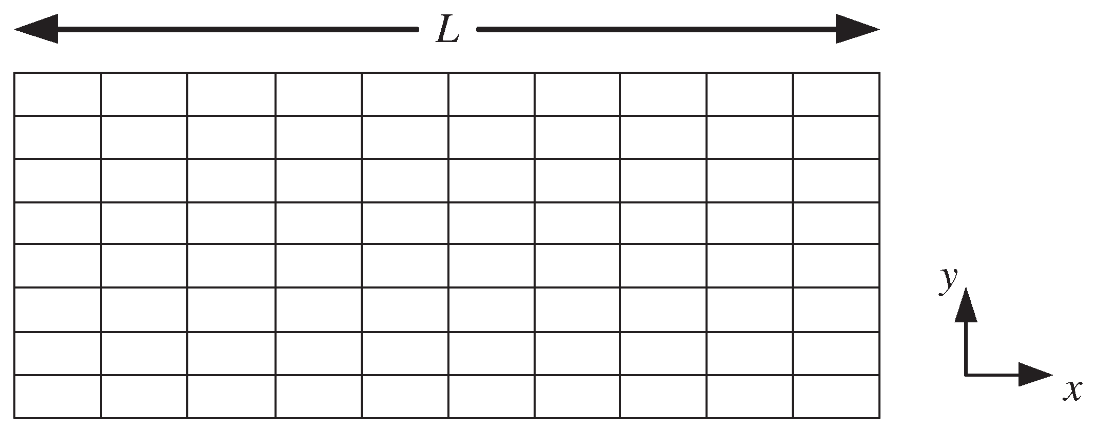
4.1. Parameter Studies with a 2D Shot Sleeve
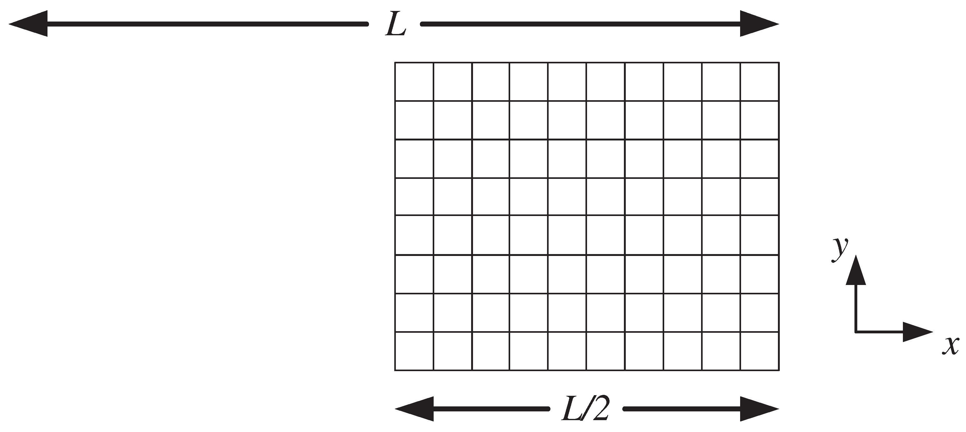
4.2. Application to a 3D Shot Sleeve
5. Conclusions
Author Contributions
Funding
Institutional Review Board Statement
Informed Consent Statement
Data Availability Statement
Conflicts of Interest
Appendix A. Mesh Motion Strategies


References
- Nogowizin, B. Theorie und Praxis des Druckgusses, 1st ed.; Schiele und Schoen: Berlin, Germany, 2010. [Google Scholar]
- Brunnhuber, E. Praxis der Druckgussfertigung; Schiele und Schoen: Berlin, Germany, 1991. [Google Scholar]
- Kaufmann, H.; Uggowitzer, P. Metallurgy and Processing of High-Integrity Light Metal Pressure Castings; Fachverlag Schiele & Schön: Berlin, Germany, 2014. [Google Scholar]
- Campbell, J. Complete Casting Handbook: Metal Casting Processes, Metallurgy, Techniques and Design; Elsevier: Amsterdam, The Netherlands, 2015. [Google Scholar]
- Garber, L. Theoretical analysis and experimental observation of air entrapment during cold chamber filling. Die Cast. Eng. 1982, 26, 14–15. [Google Scholar]
- Tszeng, T.; Chu, Y. A study of wave formation in shot sleeve of a die casting machine. J. Eng. Ind. 1994, 116, 175–182. [Google Scholar] [CrossRef]
- Zamora, R.; Faura, F.; López, J.; Hernández, J. Experimental verification of numerical predictions for the optimum plunger speed in the slow phase of a high-pressure die casting machine. Int. J. Adv. Manuf. Tech. 2007, 33, 266–276. [Google Scholar] [CrossRef]
- Fiorese, E.; Richiedei, D.; Bonollo, F. Improving the quality of die castings through optimal plunger motion planning: Analytical computation and experimental validation. Int. J. Adv. Manuf. Tech. 2017, 88, 1475–1484. [Google Scholar] [CrossRef]
- López, J.; Hernández, J.; Faura, F.; Trapaga, G. Shot sleeve wave dynamics in the slow phase of die casting injection. J. Fluids Eng. 2000, 122, 349–356. [Google Scholar] [CrossRef]
- Faura, F.; López, J.; Hernández, J. On the optimum plunger acceleration law in the slow shot phase of pressure die casting machines. Int. J. Mach. Tools Manuf. 2001, 41, 173–191. [Google Scholar] [CrossRef]
- Hernández, J.; López, J.; Faura, F.; Gómez, P. Analysis of the flow in a high-pressure die-casting injection chamber. J. Fluids Eng. 2003, 125, 315–324. [Google Scholar] [CrossRef]
- López, J.; Faura, F.; Hernández, J.; Gómez, P. On the critical plunger speed and three-dimensional effects in high-pressure die casting injection chambers. J. Manuf. Sci. Eng. Trans. ASME 2003, 125, 529–537. [Google Scholar] [CrossRef]
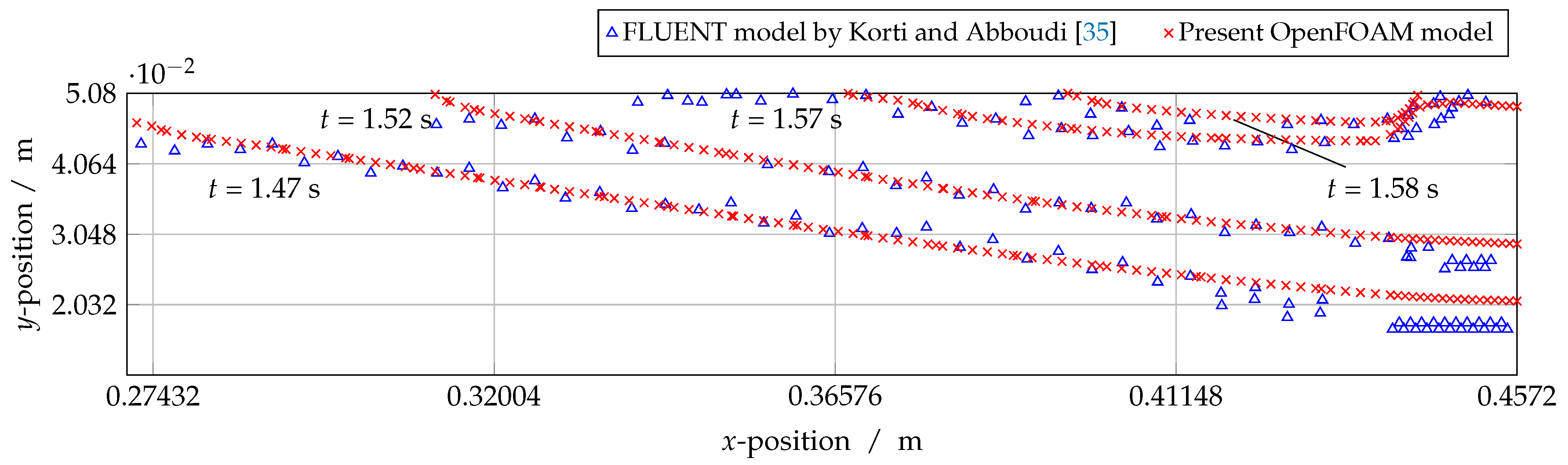
- Korti, M.C.; Korti, A.I.N.; Abboudi, S. Effects of shot sleeve filling in HPDC machine. Multidiscip. Model. Mater. Struct. 2019, 15, 1255–1273. [Google Scholar]
- Korti, A.I.N.; Abboudi, S. Effects of shot sleeve filling on evolution of the free surface and solidification in the high-pressure die casting machine. Int. J. Met. 2017, 11, 223–239. [Google Scholar] [CrossRef]
- Korti, A.I.N.; Korti, M.C.; Abboudi, S. Thermal effect in minimizing air entrainment in the 3D shot sleeve during injection stage of the HPDC machine. Int. J. Fluid Mech. Res. 2016, 43, 1–17. [Google Scholar] [CrossRef]
- Barkhudarov, M.R. Minimizing air entrainment in a shot sleeve during slow-shot stage. Die Cast. Eng. 2009, 53, 34–37. [Google Scholar]
- Nikroo, A.J.; Akhlaghi, M.; Najafabadi, M.A. Simulation and analysis of flow in the injection chamber of die casting machine during the slow shot phase. Int. J. Adv. Manuf. Tech. 2009, 41, 31–41. [Google Scholar] [CrossRef]
- Kohlstädt, S.; Vynnycky, M.; Neubauer, A.; Gebauer-Teichmann, A. Comparative RANS turbulence modelling of lost salt core viability in high pressure die casting. Prog. Comp. Fluid Dyn. 2019, 19, 316–327. [Google Scholar] [CrossRef]
- Han, T.H.; Kuo, J.H.; Hwang, W.S. Numerical simulation of the liquid-gas interface shape in the shot sleeve of cold chamber die casting machine. J. Mater. Eng. Perform. 2007, 16, 521–526. [Google Scholar] [CrossRef]
- Jasak, H.; Jemcov, A.; Tukovic, Z. OpenFOAM: A C++ Library for Complex Physics Simulations. In Proceedings of the International Workshop on Coupled Methods in Numerical Dynamics IUC, Dubrovnik, Croatia, 19–21 September 2007; pp. 1–20. [Google Scholar]
- Weller, H.; Tabor, G.; Jasak, H.; Fureby, C. A tensorial approach to computational continuum mechanics using object orientated techniques. Comput. Phys. 1998, 12, 620–631. [Google Scholar] [CrossRef]
- Jasak, H. OpenFOAM: Open source CFD in research and industry. Int. J. Nav. Archit. Ocean Eng. 2009, 1, 89–94. [Google Scholar]
- Kohlstädt, S.; Vynnycky, M.; Goeke, S. On the CFD modelling of slamming of the metal melt in high pressure die casting involving lost cores. Metals 2021, 11, 78. [Google Scholar] [CrossRef]
- Kohlstädt, S.; Vynnycky, M.; Neubauer, A.; Jäckel, J. Towards the modelling of fluid-structure interactive lost core deformation in high-pressure die casting. Appl. Math. Mod. 2020, 90, 319–333. [Google Scholar] [CrossRef]
- Kohlstädt, S.; Vynnycky, M.; Gebauer-Teichmann, A. Experimental and numerical CHT-investigations of cooling structures formed by lost cores in cast housings for optimal heat transfer. Heat Mass Trans. 2018, 54, 3445–3459. [Google Scholar] [CrossRef]
- Hirt, C.W.; Nichols, B.D. Volume of fluid (VOF) method for the dynamics of free boundaries. J. Comput. Phys. 1981, 39, 201–225. [Google Scholar] [CrossRef]
- Ferrer, P.; Causon, D.; Qian, L.; Mingham, C.; Ma, Z. A multi-region coupling scheme for compressible and incompressible flow solvers for two-phase flow in a numerical wave tank. Comput. Fluids 2016, 125, 116–129. [Google Scholar] [CrossRef] [Green Version]
- Mayon, R.; Sabeur, Z.; Tan, M.Y.; Djidjeli, K. Free surface flow and wave impact at complex solid structures. In Proceedings of the 12th International Conference on Hydrodynamics, Egmond aan Zee, The Netherlands, 18–23 September 2016; p. 10. [Google Scholar]
- Brackbill, J.; Kothe, D.; Zemach, C. A continuum method for modeling surface tension. J. Comput. Phys. 1992, 100, 335–354. [Google Scholar] [CrossRef]
- Rusche, H. Computational Fluid Dynamics of Dispersed Two-Phase Flows at High Phase Fractions. Ph.D. Thesis, Imperial College London, London, UK, 2003. [Google Scholar]
- Versteeg, H.; Malalasekera, W. An Introduction to Computational Fluid Dynamics: The Finite Volume Method, 2nd ed.; Pearson Education Limited: Harlow, UK, 2007. [Google Scholar]
- Menter, F. 2-equation eddy-viscosity turbulence models for engineering applications. AIAA J. 1994, 32, 1598–1605. [Google Scholar] [CrossRef] [Green Version]
- Robertson, E.; Choudhury, V.; Bhushan, S.; Walters, D. Validation of OpenFOAM numerical methods and turbulence models for incompressible bluff body flows. Comput. Fluids 2015, 123, 122–145. [Google Scholar] [CrossRef]
- Menter, F.R.; Kuntz, M.; Langtry, R. Ten Years of Industrial Experience with the SST Turbulence Model. Turbul. Heat Mass Transf. 2003, 4, 625–632. [Google Scholar]
- Korti, A.I.N.; Abboudi, S. Numerical simulation of the interface molten metal air in the shot sleeve chambre and mold cavity of a die casting machine. Heat Mass Transf. 2011, 47, 1465–1478. [Google Scholar] [CrossRef]
- Koch, M.; Lechner, C.; Reuter, F.; Köhler, K.; Mettin, R.; Lauterborn, W. Numerical modeling of laser generated cavitation bubbles with the finite volume and volume of fluid method, using OpenFOAM. Comput. Fluids 2016, 126, 71–90. [Google Scholar] [CrossRef]
- White, F. Fluid Mechanics, in SI Units; McGraw-Hill: New York, NY, USA, 2011. [Google Scholar]
- Patankar, S.; Spalding, D. A calculation procedure for heat, mass and momentum transfer in three-dimensional parabolic flows. In Numerical Prediction of Flow, Heat Transfer, Turbulence and Combustion; Elsevier: Amsterdam, The Netherlands, 1983; pp. 54–73. [Google Scholar]
- Issa, R. Solution of the implicitly discretised fluid flow equations by operator-splitting. J. Comput. Phys. 1986, 62, 40–65. [Google Scholar] [CrossRef]
- Gómez, P.; Hernández, J.; López, J.; Faura, F. Numerical simulation of free surface flows in die casting injection processes. Phoenics J. Comput. Fluid Dyn. 2000, 13, 186–203. [Google Scholar]
- Landau, L.D.; Lifshitz, E.M. Fluid Mechanics; Pergamon Press: Oxford, UK, 1959. [Google Scholar]
- Acheson, D.J. Elementary Fluid Dynamics; Oxford University Press: Oxford, UK, 1990. [Google Scholar]
- Reikher, A.; Barkhudarov, M. Casting: An Analytical Approach; Springer Science & Business Media: Berlin/Heidelberg, Germany, 2007. [Google Scholar]
- Karni, Y. Selection of Process Variables for Die Casting. Ph.D. Thesis, The Ohio State University, Columbus, OH, USA, 1991. [Google Scholar]
- Duran, M.; Karni, Y.; Brevick, J.; Chu, Y.; Altan, T. Minimization of Air Entrapment in the Shot Sleeve of a Die Casting Machine to Reduce Porosity; Technical Report; The Ohio State University: Columbus, OH, USA, 1991. [Google Scholar]


| Symbol | Value | Units |
|---|---|---|
| 720 | J kg K | |
| 1000 | J kg K | |
| 0.026 | W m K | |
| 70 | W m K | |
| M | 0.028 | kg mol |
| 293 | K | |
| 823 | K | |
| 1.8 × | Pa s | |
| 1.62 × 10 | Pa s | |
| 2520 | kg m | |
| 0.629 | N m |
Publisher’s Note: MDPI stays neutral with regard to jurisdictional claims in published maps and institutional affiliations. |
© 2021 by the authors. Licensee MDPI, Basel, Switzerland. This article is an open access article distributed under the terms and conditions of the Creative Commons Attribution (CC BY) license (https://creativecommons.org/licenses/by/4.0/).
Share and Cite
Kohlstädt, S.; Vynnycky, M.; Goeke, S.; Gebauer-Teichmann, A. On Determining the Critical Velocity in the Shot Sleeve of a High-Pressure Die Casting Machine Using Open Source CFD. Fluids 2021, 6, 386. https://doi.org/10.3390/fluids6110386
Kohlstädt S, Vynnycky M, Goeke S, Gebauer-Teichmann A. On Determining the Critical Velocity in the Shot Sleeve of a High-Pressure Die Casting Machine Using Open Source CFD. Fluids. 2021; 6(11):386. https://doi.org/10.3390/fluids6110386
Chicago/Turabian StyleKohlstädt, Sebastian, Michael Vynnycky, Stephan Goeke, and Andreas Gebauer-Teichmann. 2021. "On Determining the Critical Velocity in the Shot Sleeve of a High-Pressure Die Casting Machine Using Open Source CFD" Fluids 6, no. 11: 386. https://doi.org/10.3390/fluids6110386