
River Flow Measurements Utilizing UAV-Based Surface Velocimetry and Bathymetry Coupled with Sonar


Abstract
:1. Introduction
2. Materials and Methods
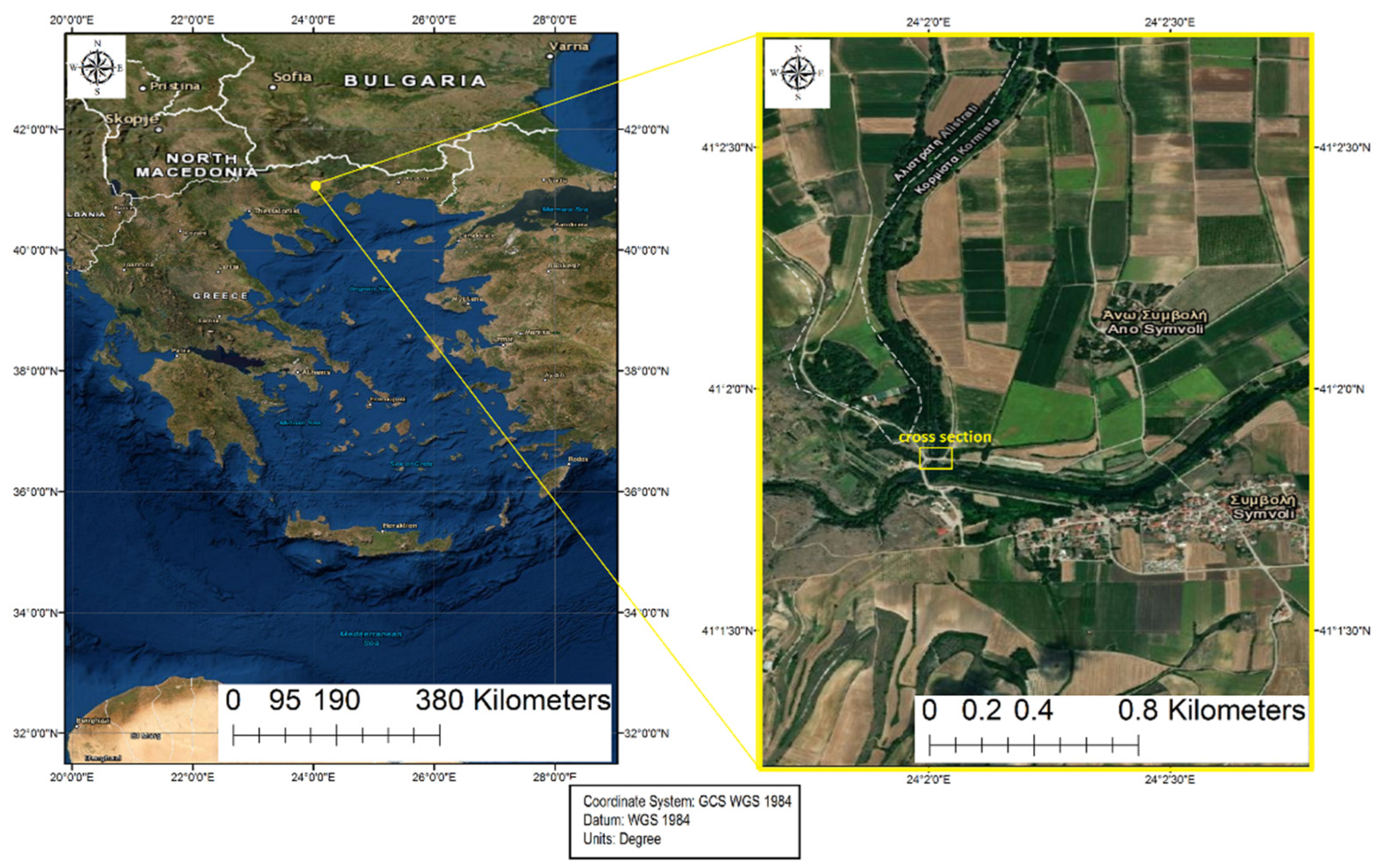
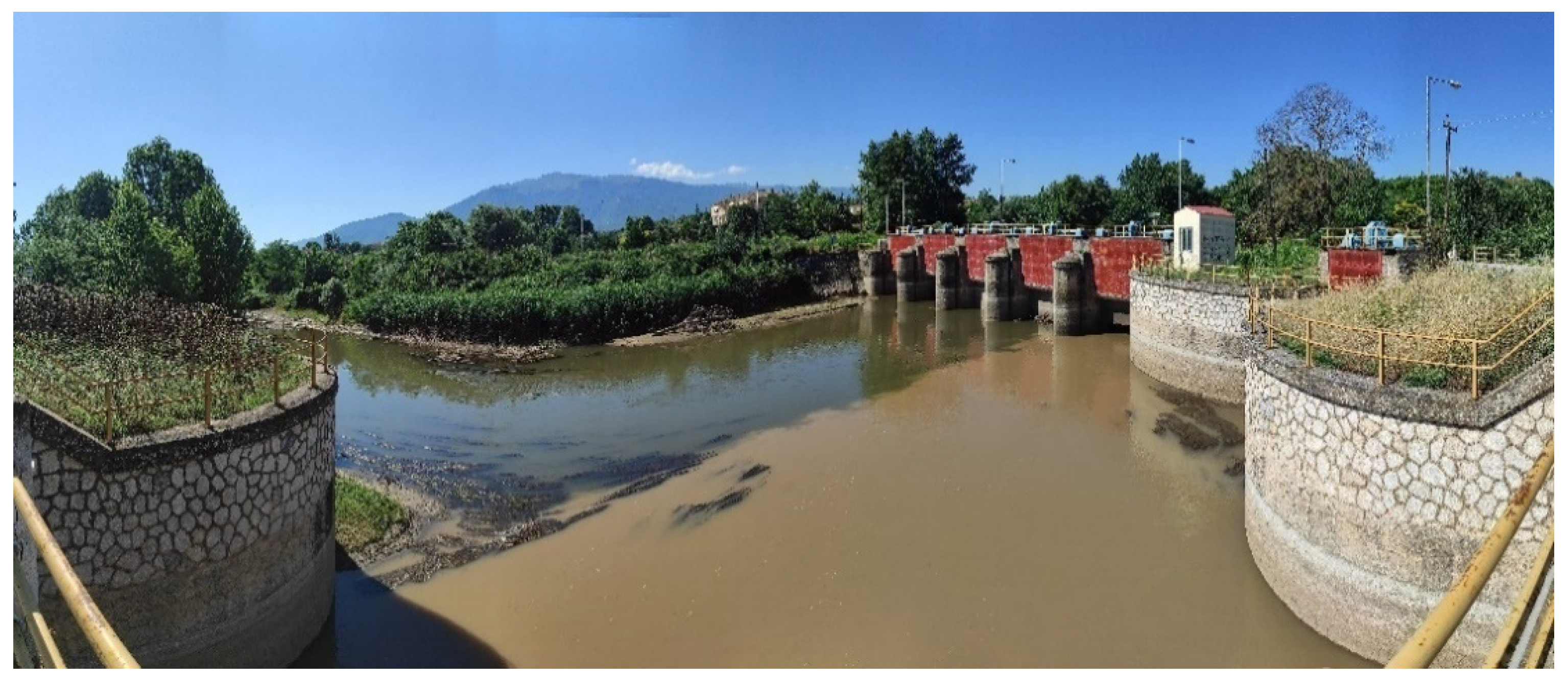
2.1. The Study Site
2.2. The Innovative Method
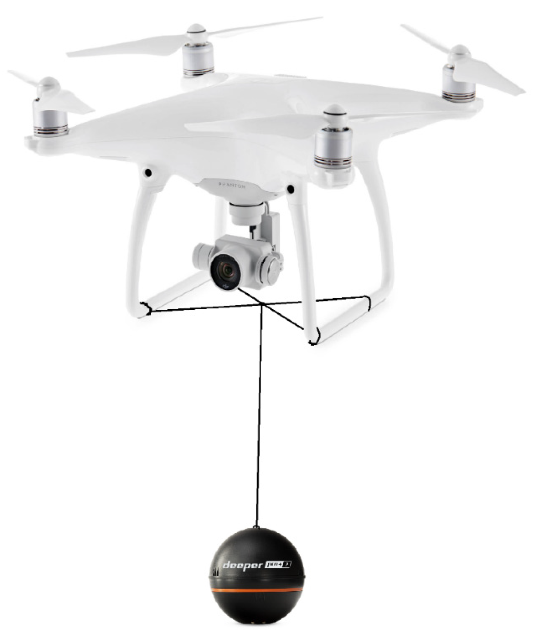
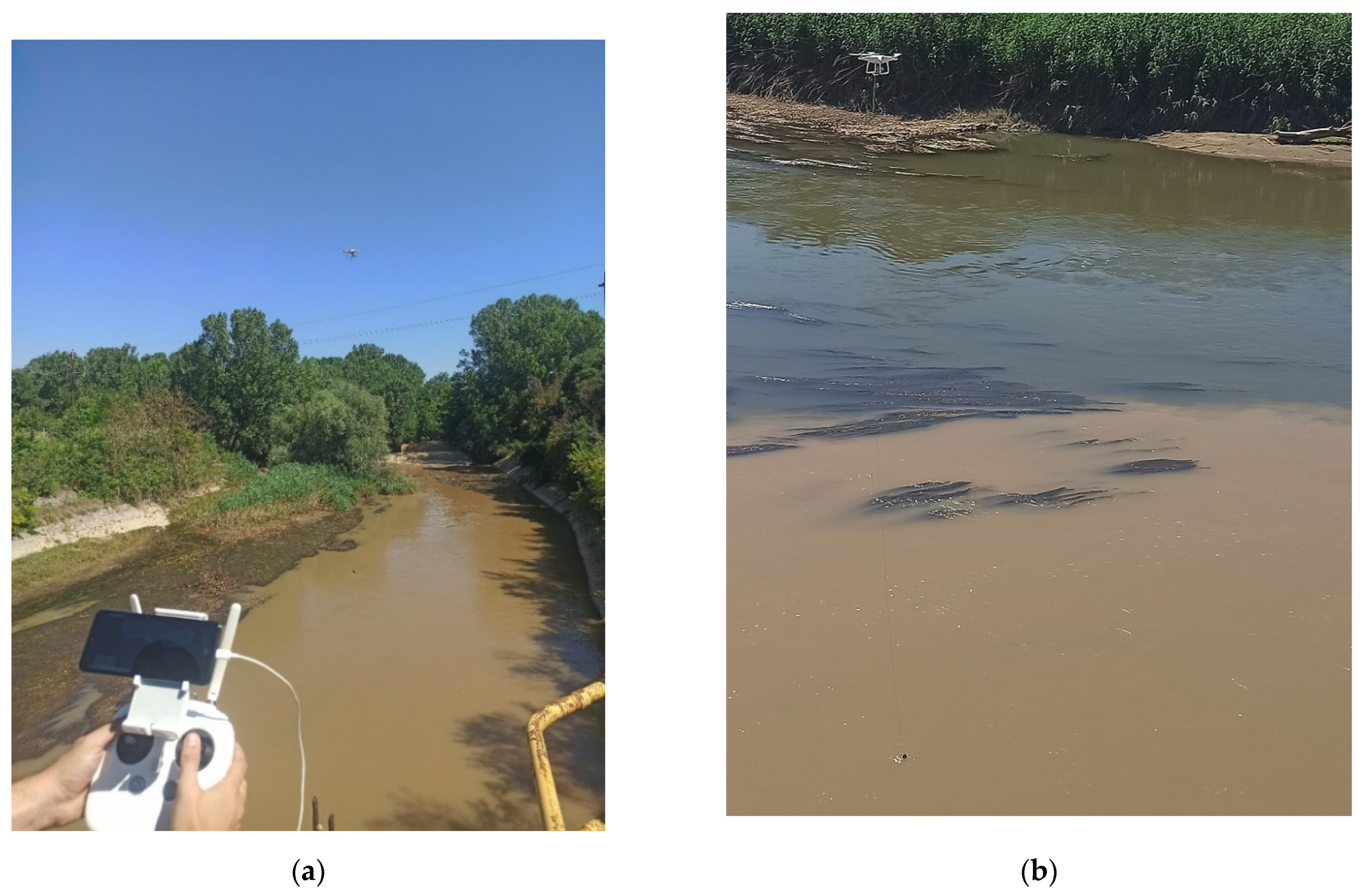
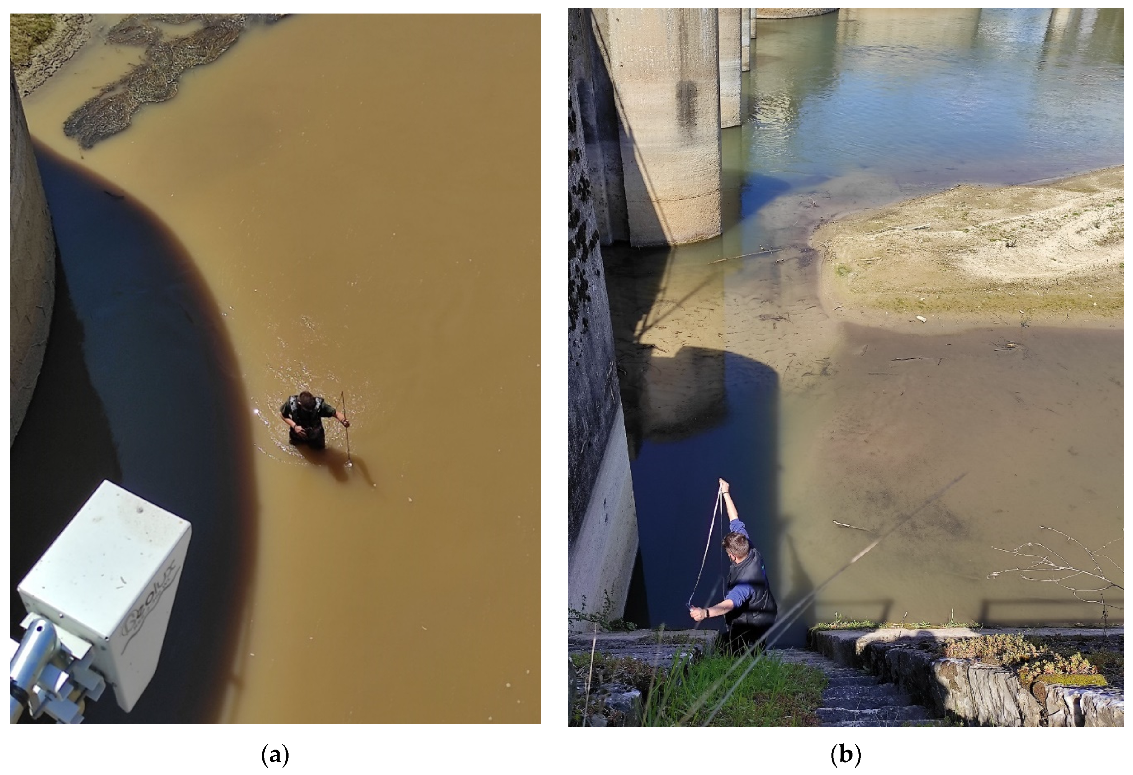
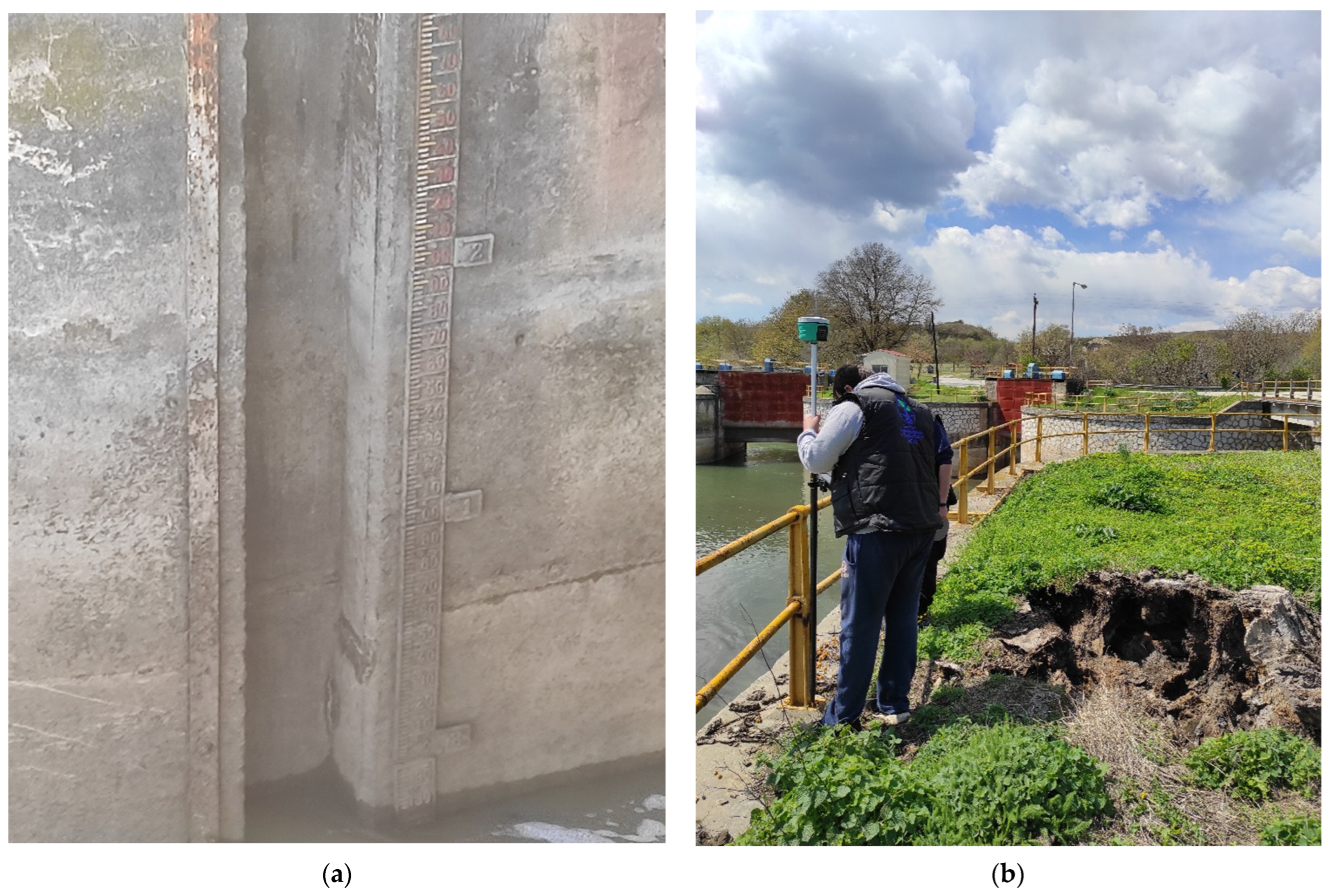
2.2.1. The Hardware
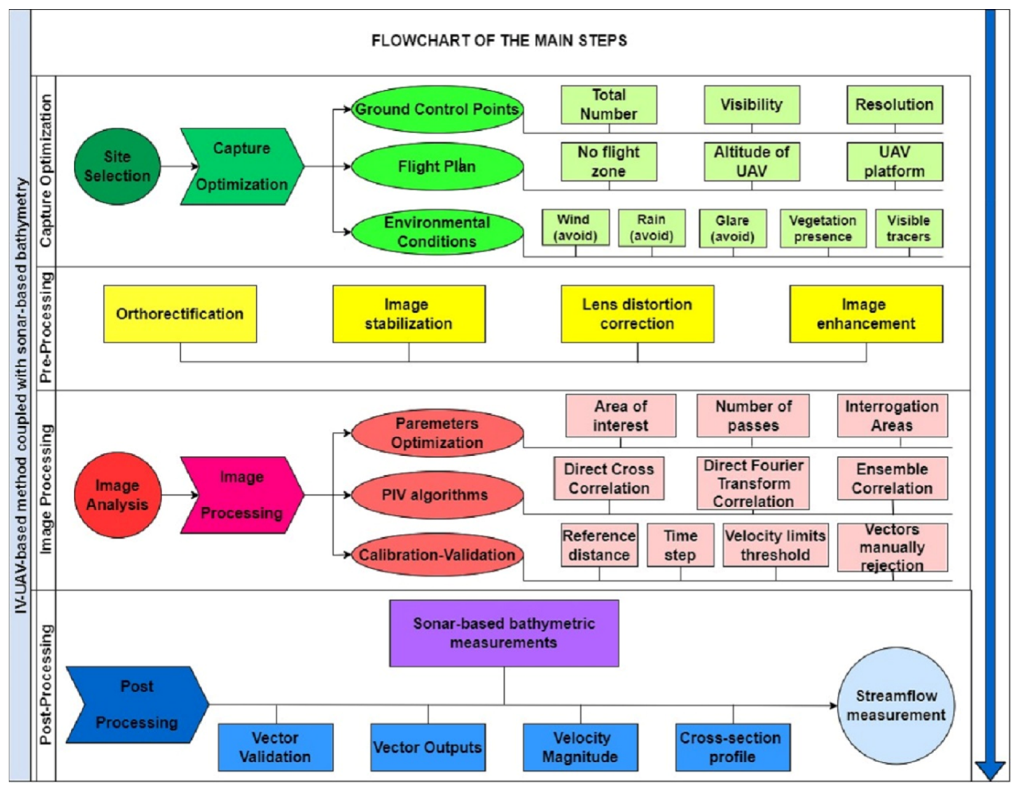
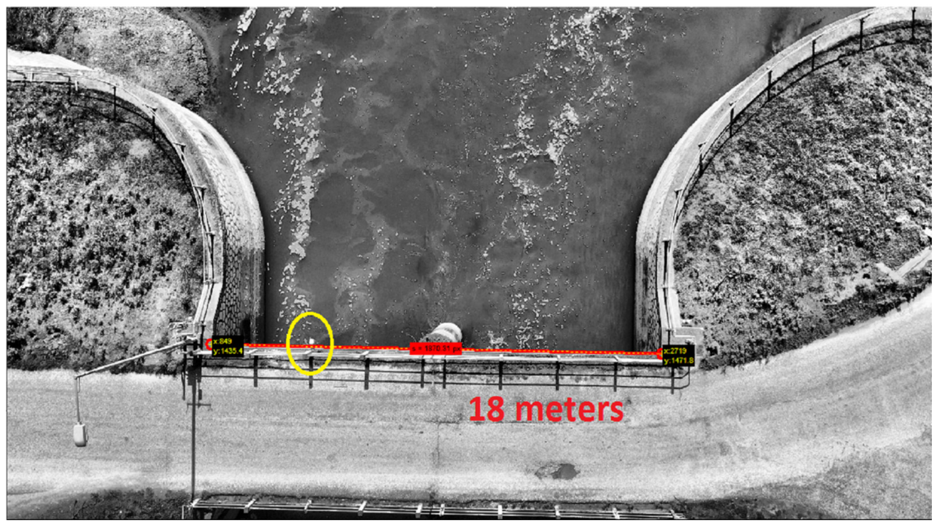
2.2.2. The Software
3. Results
4. Discussion and Recommendations
Author Contributions
Funding
Institutional Review Board Statement
Informed Consent Statement
Data Availability Statement
Acknowledgments
Conflicts of Interest
References
- Zaimes, G.N. Mediterranean riparian areas–climate change implications and recommendations. J. Environ. Biol. 2020, 41, 957–965. [Google Scholar] [CrossRef]
- Zaimes, G.N.; Iakovoglou, V.; Syropoulos, D.; Kaltsas, D.; Avtzis, D. Assessment of Two Adjacent Mountainous Riparian Areas along Nestos River Tributaries of Greece. Forests 2021, 12, 1284. [Google Scholar] [CrossRef]
- Pumo, D.; Noto, L.V.; Viola, F. Ecohydrological modelling of flow duration curve in Mediterranean river basins. Adv. Water Resour. 2013, 52, 314–327. [Google Scholar] [CrossRef]
- Burgi, P.H. Hydraulic design of vertical stilling wells. J. Hydraul. Div. 1975, 101, 801–816. [Google Scholar] [CrossRef]
- Parshall, R.L. The improved Venturi flume. Trans. Am. Soc. Civil Eng. 1926, 89, 841–851. [Google Scholar] [CrossRef]
- Mansour, H.A.; Abdallah, E.F.; Gaballah, M.S.; Gyuricza, C. Impact of bubbler discharge and irrigation water quantity on 1-hydraulic performance evaluation and maize biomass yield. Int. J. GEOMATE 2015, 9, 1538–1544. [Google Scholar] [CrossRef]
- Lamine, B.O.M.; Ferreira, V.G.; Yang, Y.; Ndehedehe, C.E.; He, X. Estimation of the Niger River cross-section and discharge from remotely-sensed products. J. Hydrol. Reg. Stud. 2021, 36, 100862. [Google Scholar] [CrossRef]
- Pantelakis, D.; Doulgeris, C.; Hatzigiannakis, E.; Arampatzis, G. Evaluation of discharge measurements methods in a natural river of low or middle flow using an electromagnetic flow meter. River Res. Appl. 2022, 38, 1003–1013. [Google Scholar] [CrossRef]
- Morlot, T.; Perret, C.; Favre, A.C.; Jalbert, J. Dynamic rating curve assessment for hydrometric stations and computation of the associated uncertainties: Quality and station management indicators. J. Hydrol. 2014, 517, 173–186. [Google Scholar] [CrossRef]
- Westerberg, I.; Guerrero, J.L.; Seibert, J.; Beven, K.J.; Halldin, S. Stage-discharge uncertainty derived with a non-stationary rating curve in the Choluteca River, Honduras. Hydrol. Processes 2011, 25, 603–613. [Google Scholar] [CrossRef]
- Corato, G.; Ammari, A.; Moramarco, T. Conventional point-velocity records and surface velocity observations for estimating high flow discharge. Entropy 2014, 16, 5546–5559. [Google Scholar] [CrossRef]
- Tsubaki, R.; Fujita, I.; Tsutsumi, S. Measurement of the flood discharge of a small-sized river using an existing digital video recording system. J. Hydro-Environ. Res. 2011, 5, 313–321. [Google Scholar] [CrossRef]
- De Girolamo, A.M.; Pappagallo, G.; Porto, A.L. Temporal variability of suspended sediment transport and rating curves in a Mediterranean river basin: The Celone (SE Italy). Catena 2015, 128, 135–143. [Google Scholar] [CrossRef]
- Kostaschuk, R.; Best, J.; Villard, P.; Peakall, J.; Franklin, M. Measuring flow velocity and sediment transport with an acoustic Doppler current profiler. Geomorphology 2005, 68, 25–37. [Google Scholar] [CrossRef]
- Boldt, J.A.; Oberg, K.A. Validation of streamflow measurements made with M9 and RiverRay acoustic Doppler current profilers. J. Hydraul. Eng. 2016, 142, 04015054. [Google Scholar] [CrossRef]
- Wang, X. Advances in separating effects of climate variability and human activity on stream discharge: An overview. Adv. Water Resour. 2014, 71, 209–218. [Google Scholar] [CrossRef]
- Stone, M.C.; Hotchkiss, R.H. Evaluating velocity measurement techniques in shallow streams. J. Hydraul. Res. 2007, 45, 752–762. [Google Scholar] [CrossRef]
- Fulton, J.; Ostrowski, J. Measuring real-time streamflow using emerging technologies: Radar, hydroacoustics, and the probability concept. J. Hydrol. 2008, 357, 1–10. [Google Scholar] [CrossRef]
- Costa, J.E.; Cheng, R.T.; Haeni, F.P.; Melcher, N.; Spicer, K.R.; Hayes, E.; Plant, W.; Hayes, K.; Teague, C.; Barrick, D. Use of radars to monitor stream discharge by noncontact methods. Water Resour. Res. 2006, 42. [Google Scholar] [CrossRef]
- Gleason, C.J.; Smith, L.C. Toward global mapping of river discharge using satellite images and at-many-stations hydraulic geometry. Proc. Natl. Acad. Sci. USA 2014, 111, 4788–4791. [Google Scholar] [CrossRef]
- Pavelsky, T.M. Using width-based rating curves from spatially discontinuous satellite imagery to monitor river discharge. Hydrol. Processes 2014, 28, 3035–3040. [Google Scholar] [CrossRef]
- Kastridis, A.; Stathis, D. Evaluation of hydrological and hydraulic models applied in typical Mediterranean Ungauged watersheds using post-flash-flood measurements. Hydrology 2020, 7, 12. [Google Scholar] [CrossRef]
- Papaioannou, G.; Efstratiadis, A.; Vasiliades, L.; Loukas, A.; Papalexiou, S.M.; Koukouvinos, A.; Tsoukalas, I.; Kossieris, P. An operational method for flood directive implementation in ungauged urban areas. Hydrology 2018, 5, 24. [Google Scholar] [CrossRef]
- Tosi, F.; Rocca, M.; Aleotti, F.; Poggi, M.; Mattoccia, S.; Tauro, F.; Toth, E.; Grimaldi, S. Enabling image-based streamflow monitoring at the edge. Remote Sens. 2020, 12, 2047. [Google Scholar] [CrossRef]
- Pumo, D.; Alongi, F.; Ciraolo, G.; Noto, L.V. Optical methods for river monitoring: A simulation-based approach to explore optimal experimental setup for LSPIV. Water 2021, 13, 247. [Google Scholar] [CrossRef]
- Tauro, F.; Olivieri, G.; Petroselli, A.; Porfiri, M.; Grimaldi, S. Flow monitoring with a camera: A case study on a flood event in the Tiber River. Environ. Monit. Assess. 2016, 188, 118. [Google Scholar] [CrossRef] [PubMed]
- Tauro, F. Particle tracers and image analysis for surface flow observations. Wiley Interdiscip. Rev. Water 2016, 3, 25–39. [Google Scholar] [CrossRef]
- Admiraal, D.M.; Stansbury, J.S.; Haberman, C.J. Case study: Particle velocimetry in a model of lake Ogallala. J. Hydraul. Eng. 2004, 130, 599–607. [Google Scholar] [CrossRef]
- Perks, M.T.; Fortunato Dal Sasso, S.; Hauet, A.; Jamieson, E.; Le Coz, J.; Pearce, S.; Peña-Haro, S.; Pizarro, A.; Strelnikova, D.; Tauro, F.; et al. Towards harmonisation of image velocimetry techniques for river surface velocity observations. Earth Syst. Sci. Data 2020, 12, 1545–1559. [Google Scholar] [CrossRef]
- Fujita, I.; Watanabe, H.; Tsubaki, R. Development of a non-intrusive and efficient flow monitoring technique: The space-time image velocimetry (STIV). Int. J. River Basin Manag. 2007, 5, 105–114. [Google Scholar] [CrossRef]
- Fujita, I.; Muste, M.; Kruger, A. Large-scale particle image velocimetry for flow analysis in hydraulic engineering applications. J. Hydraul. Res. 1998, 36, 397–414. [Google Scholar] [CrossRef]
- Patalano, A.; Garcia, C.M.; Brevis, W.; Bleninger, T.; Guillen, N.; Moreno, L.; Rodriguez, A. Recent advances in Eulerian and Lagragian large-scale particle image velocimetry. In Proceedings of the 36th IAHR World Congress, The Hauge, The Netherlands, 28 June–3 July 2015. [Google Scholar]
- Jolley, M.J.; Russell, A.J.; Quinn, P.F.; Perks, M.T. Considerations When Applying Large-Scale PIV and PTV for Determining River Flow Velocity. Front. Water 2021, 3, 709269. [Google Scholar] [CrossRef]
- Manfreda, S.; McCabe, M.F.; Miller, P.E.; Lucas, R.; Pajuelo Madrigal, V.; Mallinis, G.; Ben Dor, E.; Helman, D.; Estes, L.; Ciraolo, G.; et al. On the use of unmanned aerial systems for environmental monitoring. Remote Sens. 2018, 10, 641. [Google Scholar] [CrossRef]
- Whitehead, K.; Hugenholtz, C.H. Remote sensing of the environment with small unmanned aircraft systems (UASs), part 1: A review of progress and challenges. J. Unmanned Veh. Syst. 2014, 2, 69–85. [Google Scholar] [CrossRef]
- Schweitzer, S.A.; Cowen, E.A. Instantaneous River-Wide Water Surface Velocity Field Measurements at Centimeter Scales Using Infrared Quantitative Image Velocimetry. Water Resour. Res. 2021, 57, e2020WR029279. [Google Scholar] [CrossRef]
- Kinzel, P.J.; Legleiter, C.J. sUAS-based remote sensing of river discharge using thermal particle image velocimetry and bathymetric lidar. Remote Sens. 2019, 11, 2317. [Google Scholar] [CrossRef]
- Le Boursicaud, R.; Pénard, L.; Hauet, A.; Thollet, F.; Le Coz, J. Gauging extreme floods on YouTube: Application of LSPIV to home movies for the post-event determination of stream discharges. Hydrol Processes 2016, 30, 90–105. [Google Scholar] [CrossRef]
- Hauet, A.; Muste, M.; Ho, H.C. Digital mapping of riverine waterway hydrodynamic and geomorphic features. Earth Surf. Processes Landf. 2009, 34, 242–252. [Google Scholar] [CrossRef]
- Lewis, Q.W.; Rhoads, B.L. Resolving two-dimensional flow structure in rivers using large-scale particle image velocimetry: An example from a stream confluence. Water Resour. Res. 2015, 51, 7977–7994. [Google Scholar] [CrossRef]
- Kim, Y.; Muste, M.; Hauet, A.; Krajewski, W.F.; Kruger, A.; Bradley, A. Stream discharge using mobile large-scale particle image velocimetry: A proof of concept. Water Resour. Res. 2008, 44, W09502. [Google Scholar] [CrossRef]
- Tauro, F.; Petroselli, A.; Arcangeletti, E. Assessment of drone-based surface flow observations. Hydrol. Processes 2016, 30, 1114–1130. [Google Scholar] [CrossRef]
- Tauro, F.; Porfiri, M.; Grimaldi, S. Orienting the camera and firing lasers to enhance large scale particle image velocimetry for streamflow monitoring. Water Resour. Res. 2014, 50, 7470–7483. [Google Scholar] [CrossRef]
- Le Coz, J.; Hauet, A.; Pierrefeu, G.; Dramais, G.; Camenen, B. Performance of image-based velocimetry (LSPIV) applied to flash-flood discharge measurements in Mediterranean rivers. J. Hydrol. 2010, 394, 42–52. [Google Scholar] [CrossRef]
- Jodeau, M.; Bel, C.; Antoine, G.; Bodart, G.; Le Coz, J.; Faure, J.B.; Hauet, A.; Leclercq, F.; Haddad, H.; Legout, C.; et al. New developments of FUDAA-LSPIV, a user-friendly software to perform river velocity measurements in various flow conditions. In Proceedings of the 10th Conference on Fluvial Hydraulics “River Flow 2020”, Delft, The Netherlands, 6–17 July 2020. [Google Scholar]
- Dal Sasso, S.F.; Pizarro, A.; Manfreda, S. Recent Advancements and Perspectives in UAS-Based Image Velocimetry. Drones 2021, 5, 81. [Google Scholar] [CrossRef]
- Manfreda, S.; Dal Sasso, S.F.; Pizarro, A.; Tauro, F. New insights offered by UAS for river monitoring. In Applications of Small Unmanned Aircraft Systems: Best Practices and Case Studies; Sharma, J.B., Ed.; CRC Press, Taylor and Francis Group: New York, NY, USA, 2019; pp. 211–234. [Google Scholar]
- Strelnikova, D.; Paulus, G.; Käfer, S.; Anders, K.H.; Mayr, P.; Mader, H.; Scherling, U.; Schneeberger, R. Drone-based optical measurements of heterogeneous surface velocity fields around fish passages at hydropower dams. Remote Sens. 2020, 12, 384. [Google Scholar] [CrossRef]
- Koutalakis, P. Development of Image-Based Velocimetry and Methodology to Map Geomorphologic Changes on Riverbeds by Utilizing Images/Video Captured by Unmanned Aerial Vehicles. Ph.D. Thesis, University of the Aegean, Mytilene, Greece, 2021. [Google Scholar]
- Fujita, I.; Aya, S. Refinement of LSPIV technique for monitoring river surface flows. In Proceedings of the Joint Conference on Water Resource Engineering and Water Resources Planning and Management 2000: Building Partnerships, Minneapolis, MN, USA, 30 July–2 August 2000; pp. 1–9. [Google Scholar]
- Kantoush, S.A.; Schleiss, A.J.; Sumi, T.; Murasaki, M. LSPIV implementation for environmental flow in various laboratory and field cases. J. Hydro-Environ. Res. 2011, 5, 263–276. [Google Scholar] [CrossRef]
- Pearce, S.; Ljubičić, R.; Peña-Haro, S.; Perks, M.; Tauro, F.; Pizarro, A.; Dal Sasso, S.F.; Strelnikova, D.; Grimaldi, S.; Maddock, I.; et al. An evaluation of image velocimetry techniques under low flow conditions and high seeding densities using unmanned aerial systems. Remote Sens. 2020, 12, 232. [Google Scholar] [CrossRef]
- Meselhe, E.A.; Peeva, T.; Muste, M.V.I. Large scale particle image velocimetry for low velocity and shallow water flows. J. Hydrol. Eng. 2004, 130, 937–940. [Google Scholar] [CrossRef]
- Detert, M.; Weitbrecht, V. A low-cost airborne velocimetry system: Proof of concept. J. Hydraul. Res. 2015, 53, 532–539. [Google Scholar] [CrossRef]
- Tauro, F.; Piscopia, R.; Grimaldi, S. Streamflow observations from cameras: Large-scale particle image velocimetry or particle tracking velocimetry? Water Resour. Res. 2017, 53, 10374–10394. [Google Scholar] [CrossRef]
- Tauro, F.; Porfiri, M.; Grimaldi, S. Surface flow measurements from drones. J. Hydrol. 2016, 540, 240–245. [Google Scholar] [CrossRef]
- Lewis, Q.W.; Rhoads, B.L. LSPIV measurements of two-dimensional flow structure in streams using small unmanned aerial systems: 1. Accuracy assessment based on comparison with stationary camera platforms and in-stream velocity measurements. Water Resour. Res. 2018, 54, 8000–8018. [Google Scholar] [CrossRef]
- Lewis, Q.W. Measuring Flow and Mixing at Stream Confluences Using Large-Scale Particle Image Velocimetry, In-Stream Techniques, and Small Unmanned Aerial Systems. Ph.D. Thesis, University of Illinois at Urbana-Champaign, Urbana-Champaign, IL, USA, 2018. [Google Scholar]
- Huang, W.C.; Young, C.C.; Liu, W.C. Application of an automated discharge imaging system and LSPIV during typhoon events in Taiwan. Water 2018, 10, 280. [Google Scholar] [CrossRef]
- Creëlle, S.; Roldan, R.; Herremans, A.; Meire, D.; Buis, K.; Meire, P.; Van Oyen, T.; De Mulder, T.; Troch, P. Validation of large-scale particle image velocimetry to acquire free-surface flow fields in vegetated rivers. J. Appl. Water Eng. Res. 2018, 6, 171–182. [Google Scholar] [CrossRef]
- Fairley, I.; Williamson, B.J.; McIlvenny, J.; King, N.; Masters, I.; Lewis, M.; Neill, S.; Glasby, D.; Coles, D.; Powel, B.; et al. Drone-based large-scale particle image velocimetry applied to tidal stream energy resource assessment. Renew. Energy 2022, 196, 839–855. [Google Scholar] [CrossRef]
- Lewis, Q.W.; Lindroth, E.M.; Rhoads, B.L. Integrating unmanned aerial systems and LSPIV for rapid, cost-effective stream gauging. J. Hydrol. 2018, 560, 230–246. [Google Scholar] [CrossRef]
- Kantoush, S.A.; Schleiss, A.J. Large-scale PIV surface flow measurements in shallow basins with different geometries. J. Vis. 2009, 12, 361–373. [Google Scholar] [CrossRef]
- Shi, Y. Smart cameras for machine vision. In Smart Cameras; Belbachir, A.N., Ed.; Springer: Boston, MA, USA, 2009; pp. 283–303. [Google Scholar]
- Dal Sasso, S.F.; Pizarro, A.; Pearce, S.; Maddock, I.; Manfreda, S. Increasing LSPIV performances by exploiting the seeding distribution index at different spatial scales. J. Hydrol. 2021, 598, 126438. [Google Scholar] [CrossRef]
- Mandlburger, G. Bathymetry from images, LiDAR, and Sonar. PFG–J. Photogramm. Remote Sens. Geoinf. Sci. 2021, 89, 69–70. [Google Scholar] [CrossRef]
- Bandini, F.; Kooij, L.; Mortensen, B.K.; Caspersen, M.B.; Olesen, D.; Bauer-Gottwein, P. Mapping inland water bathymetry with Ground Penetrating Radar (GPR) on board Unmanned Aerial Systems (UASs). Res. Sq. 2021. Preprints.. [Google Scholar] [CrossRef]
- Lin, Y.C.; Ho, H.C.; Lee, T.A.; Chen, H.Y. Application of Image Tech-nique to Obtain Surface Velocity and Bed Elevation in Open-Channel Flow. Water 2022, 14, 1895. [Google Scholar] [CrossRef]
- Rossi, L.; Mammi, I.; Pelliccia, F. UAV-derived multispectral bathymetry. Remote Sens. 2020, 12, 3897. [Google Scholar] [CrossRef]
- Matsuba, Y.; Sato, S. Nearshore bathymetry estimation using UAV. Coast. Eng. 2018, 60, 51–59. [Google Scholar] [CrossRef]
- Sanjou, M.; Kato, K.; Aizawa, W.; Okamoto, T. Development of drone-type float for surface-velocity measurement in rivers. Environ. Fluid Mech. 2022, 22, 955–969. [Google Scholar] [CrossRef]
- Lubczonek, J.; Kazimierski, W.; Zaniewicz, G.; Lacka, M. Methodology for combining data acquired by unmanned surface and aerial vehicles to create digital bathymetric models in shallow and ultra-shallow waters. Remote Sens. 2021, 14, 105. [Google Scholar] [CrossRef]
- Erena, M.; Atenza, J.F.; García-Galiano, S.; Domínguez, J.A.; Bernabé, J.M. Use of drones for the topo-bathymetric monitoring of the reservoirs of the Segura River Basin. Water 2019, 11, 445. [Google Scholar] [CrossRef]
- Zinke, P.; Flener, C. Experiences from the use of unmanned aerial vehicles (UAV) for river bathymetry modelling in Norway. Vann 2013, 48, 351–360. [Google Scholar]
- Bandini, F.; Olesen, D.; Jakobsen, J.; Kittel, C.M.M.; Wang, S.; Garcia, M.; Bauer-Gottwein, P. Bathymetry observations of inland water bodies using a tethered sing-beam sonar controlled by an Unmanned Aerial Vehicle. Hydrol. Earth Syst. Sci. 2008, 25, 4549–4565. [Google Scholar]
- Ruffell, A.; Lally, A.; Rocke, B. Dronar—Geoforensic Search Sonar from a Drone. Forensic Sci. 2021, 1, 202–212. [Google Scholar] [CrossRef]
- Bandini, F.; Bauer-Gottwein, P.; Garcia, M. Hydraulics and Drones: Observations of Water Level, Bathymetry and Water Surface Velocity from Unmanned Aerial Vehicles. Ph.D. Thesis, Technical Univerity of Denmark, Lyngby, Denmark, 2017. [Google Scholar]
- Astaras, T. The Gorge of the Angitis River at “Stena Petras” Near the Alistrati Cave. A Magnificent Piece of Natural Architecture in Eastern Macedonia, Greece. In Natural Heritage from East to West: Case Studies from 6 Countries; Evelpidou, N., de Figueiredo, T., Mauro, F., Tecim, V., Vassilopoulos, A., Eds.; Springer: Berlin/Heidelberg, Germany, 2010; pp. 51–57. [Google Scholar]
- Koutalakis, P.; Tzoraki, O.; Zaimes, G.N. Detecting riverbank changes with remote sensing tools. Case study: Aggitis River in Greece. Ann. Dunarea Jos Univ. Galati Fascicle II Math. Phys. Theor. Mech. 2019, 42, 134–142. [Google Scholar] [CrossRef]
- Pennos, C.; Lauritzen, S.E.; Pechlivanidou, S.; Sotiriadis, Y. Geomorphic constrains on the evolution of the Aggitis River Basin Northern Greece (a preliminary report). BGSG 2016, 50, 365–373. [Google Scholar] [CrossRef]
- Georgakopoulos, A.; Fernández-Turiel, J.; Christanis, K.; Kalaitzidis, S.; Kasso-li-Fournaraki, A.; Llorens, J.; Filippidis, A.; Gimeno, D. The Drama basin water: Quality and peat/lignite interaction. Environ. Geol. 2001, 41, 121–127. [Google Scholar] [CrossRef]
- Schismenos, S.; Stevens, G.J.; Georgeou, N.; Emmanouloudis, D.; Shrestha, S.; Thapa, B.S.; Gurung, S. Flood and Renewable Energy Humanitarian Engineering Research: Lessons from Aggitis, Greece and Dhuskun, Nepal. Geosci. J. 2022, 12, 71. [Google Scholar] [CrossRef]
- Bartzoudis, G. The Hydraulic Works in the Plain of Serres, Greece; Reprint March 2021; Serres, Greece, 1994. (In Greek)
- Liu, W.C.; Lu, C.H.; Huang, W.C. Large-scale particle image velocimetry to measure streamflow from videos recorded from unmanned aerial vehicle and fixed imaging system. Remote Sens. 2021, 13, 2661. [Google Scholar] [CrossRef]
- DJI Phantom Pro Specifications. Available online: https://www.dji.com (accessed on 24 May 2022).
- Bogoyavlensky, V.; Bogoyavlensky, I.; Nikonov, R.; Kishankov, A. Complex of geophysical studies of the Seyakha catastrophic gas blowout crater on the Yamal Peninsula, Russian Arctic. Geosci. J. 2020, 10, 215. [Google Scholar] [CrossRef]
- Maiakovska, O.; Andriantsoa, R.; Tönges, S.; Legrand, C.; Gutekunst, J.; Hanna, K.; Pârvulescu, L.; Novitsky, R.; Weiperth, A.; Sciberras, A.; et al. Genome analysis of the monoclonal marbled crayfish reveals genetic separation over a short evolutionary timescale. Commun. Biol. 2021, 4, 74. [Google Scholar] [CrossRef]
- Giambastiani, Y.; Giusti, R.; Cecchi, S.; Palomba, F.; Manetti, F.; Romanelli, S.; Bottai, L. Volume estimation of lakes and reservoirs based on aquatic drone surveys: The case study of Tuscany, Italy. J. Water Land Dev. 2020, 46, 84–96. [Google Scholar]
- Szlapińska, S.; Tokarczyk, R. A Comparison of Accuracy between Point Clouds from Convergent Images and Spherical Panoramas. Geomat. Environ. Eng. 2017, 11, 63–72. [Google Scholar] [CrossRef]
- Fang, W.; Zheng, L. Distortion correction modeling method for zoom lens cameras with bundle adjustment. J. Opt. Soc. Korea 2016, 20, 140–149. [Google Scholar] [CrossRef]
- Hedborg, J.; Ringaby, E.; Forssén, P.E.; Felsberg, M. Structure and motion estimation from rolling shutter video. In Proceedings of the IEEE International Conference on Computer Vision Workshops (ICCV Workshops), Barcelona, Spain, 6–13 November 2011; pp. 17–23. [Google Scholar]
- Tsai, T.H.; Fang, C.L.; Chuang, H.M. Design and implementation of efficient video stabilization engine using maximum a posteriori estimation and motion energy smoothing approach. IEEE Trans. Circuits Syst. Video Technol. 2011, 22, 817–830. [Google Scholar] [CrossRef]
- Walha, A.; Wali, A.; Alimi, A.M. Video stabilization with moving object detecting and tracking for aerial video surveillance. Multimed. Tools Appl. 2015, 74, 6745–6767. [Google Scholar] [CrossRef]
- Koutalakis, P.; Tzoraki, O.; Zaimes, G.N. Software utilized for image-based velocimetry methods focused on water resources. Desalin. Water Treat. 2021, 218, 1–17. [Google Scholar] [CrossRef]
- Thielicke, W.; Stamhuis, E. PIVlab—Towards user-friendly, affordable and accurate digital particle image velocimetry in MATLAB. J. Open Res. Softw. 2014, 2, p.e30. [Google Scholar] [CrossRef]
- Koutalakis, P.; Tzoraki, O.; Zaimes, G. UAVs for hydrologic scopes: Application of a low-cost UAV to estimate surface water velocity by using three different image-based methods. Drones 2019, 3, 14. [Google Scholar] [CrossRef]
- Cao, L.; Weitbrecht, V.; Li, D.; Detert, M. Airborne Feature Matching Velocimetry for surface flow measurements in rivers. J. Hydraul. Res. 2021, 59, 637–650. [Google Scholar] [CrossRef]
- Patalano, A.; García, C.M. RIVeR—Towards affordable, practical and user-friendly toolbox for Large Scale PIV and PTV techniques. In Proceedings of the International Conference on Fluvial Hydraulics “River Flow 2016”, St. Louis, MO, USA, 11–14 July 2016; pp. 576–579. [Google Scholar]
- Ioli, F.; Pinto, L.; Passoni, D.; Nova, V.; Detert, M. Evaluation of Airborne Image Velocimetry approaches using low-cost UAVs in riverine environments. Int. Arch. Photogramm. Remote Sens. Spat. Inf. Sci.—ISPRS Arch. 2020, 43, 597–604. [Google Scholar] [CrossRef]
- Gore, J.A.; Banning, J. Chapter 3—Discharge measurements and streamflow analysis. In Methods in Stream Ecology, 3rd ed.; Hauer, F.R., Lamberti, G.A., Eds.; Academic Press: Cambridge, MA, USA, 1996; pp. 49–70. [Google Scholar]
- Gravelle, R. Discharge estimation: Techniques and equipment. In Geomorphological Techniques; (Online Edition), Chapter: 3.3.5; Clarke, L.E., Nield, J.M., Eds.; British Society for Geomorphology: London, UK, 2015; Volume 5, pp. 1–8. [Google Scholar]
- Ferguson, R.I.; Parsons, D.R.; Lane, S.N.; Hardy, R.J. Flow in meander bends with recirculation at the inner bank. Water Resour. Res. 2003, 39. [Google Scholar] [CrossRef]
- Nilsson, C. Distribution of stream-edge vegetation along a gradient of current velocity. J. Ecol. 1987, 75, 513–522. [Google Scholar] [CrossRef]
- Huang, H.Q.; Nanson, G.C. Vegetation and channel variation; a case study of four small streams in southeastern Australia. Geomorphology 1997, 18, 237–249. [Google Scholar] [CrossRef]
- Gran, K.; Paola, C. Riparian vegetation controls on braided stream dynamics. Water Resour. Res. 2001, 37, 3275–3283. [Google Scholar] [CrossRef]
- Beschta, R.L.; Platts, W.S. Morphological Features of Small Streams: Significance and Function. J. Am. Water Resour. Assoc. 1986, 22, 369–379. [Google Scholar] [CrossRef]
- Bell, J.M.; Simonson, A.M.; Fisher, I.J. Urban Hydrology—Science Capabilities of the U.S. Geological Survey; Northeast Region Urban Landscape Capabilities Team; Fact Sheet 2016-3023; U.S. Geological Survey: Reston, VA, USA, 2016. [CrossRef]
- Hohensinner, S.; Hauer, C.; Muhar, S. River morphology, channelization, and habitat restoration. Riverine ecosystem management. In Riverine Ecosystem Management; Schmutz, S., Sendzimirpringer, J., Eds.; Springer: Cham, Switzerland, 2018; pp. 41–65. [Google Scholar]
- Zaimes, G.N.; Gounaridis, D.; Symenonakis, E. Assessing the impact of dams on riparian and deltaic vegetation using remotely-sensed vegetation indices and Random Forests modelling. Ecol. Indic. 2019, 103, 630–641. [Google Scholar] [CrossRef]
- Książek, L.; Woś, A.; Florek, J.; Wyrębek, M.; Młyński, D.; Wałęga, A. Combined use of the hydraulic and hydrological methods to calculate the environmental flow: Wisloka river, Poland: Case study. Environ. Monit. Assess. 2019, 191, 254. [Google Scholar] [CrossRef] [PubMed]
- Whiting, P.J. Streamflow necessary for environmental maintenance. Annu. Rev. Earth Planet. Sci. 2002, 30, 181. [Google Scholar] [CrossRef]
- Tharme, R.E. A global perspective on environmental flow assessment: Emerging trends in the development and application of environmental flow methodologies for rivers. River Res. Appl 2003, 19, 397–441. [Google Scholar] [CrossRef]
- Merritt, D.M.; Scott, M.L.; LeRoy Poff, N.; Auble, G.T.; Lytle, D.A. Theory, methods and tools for determining environmental flows for riparian vegetation: Riparian vegetation-flow response guilds. Freshw. Biol. 2010, 55, 206–225. [Google Scholar] [CrossRef]
- Maes, J.; Jacobs, S. Nature-based solutions for Europe’s sustainable development. Conserv. Lett. 2017, 10, 121–124. [Google Scholar] [CrossRef]
- Gonzalez-Ollauri, A. Sustainable Use of Nature-Based Solutions for Slope Protection and Erosion Control. Sustainability 2022, 14, 1981. [Google Scholar] [CrossRef]
- Guerrero, P.; Haase, D.; Albert, C. Locating spatial opportunities for nature-based solutions: A river landscape application. Water 2018, 10, 1869. [Google Scholar] [CrossRef]
- Iakovoglou, V.; Koutalakis, P.; Diaconu, D.; Tufekcioglu, M.; Trombitsky, I.; Ghulijanyan, A.; Zaimes, G.N. Nature-based solutions for streams to reduce sediment and litter pollution in the Black Sea. In Proceedings of the Environmental Challenges in the Black Sea Basin: Impact on Human Health, Galati, Romania, 23–26 September 2020. [Google Scholar]
- Vogel, S. Life in Moving Fluids: The Physical Biology of Flow-Revised and Expanded, 2nd ed.; Princeton University Press: Princeton, NJ, USA, 2020; pp. 47–50. [Google Scholar]
- Strahler, A.N. Dynamic basis of geomorphology. Geol. Soc. Am. Bull. 1952, 63, 923–938. [Google Scholar] [CrossRef]
- Andreotti, B.; Claudin, P.; Devauchelle, O.; Durán, O.; Fourrière, A. Bedforms in a turbulent stream: Ripples, chevrons and antidunes. J. Fluid Mech. 2012, 690, 94–128. [Google Scholar] [CrossRef]
- Keller, E.A. Areal sorting of bed-load material: The hypothesis of velocity reversal. Geol. Soc. Am. Bull. 1971, 82, 753–756. [Google Scholar] [CrossRef]
- Kaffas, K.; Hrissanthou, V. Computation of hydro-geomorphologic changes in two basins of northeastern Greece. In Hydro-Geomorphology-Models and Trends; Shukla, D.P., Ed.; IntechOpen: London, UK, 2017; pp. 9–32. [Google Scholar]
- Rusnák, M.; Goga, T.; Michaleje, L.; Šulc Michalková, M.; Máčka, Z.; Bertalan, L.; Kidová, A. Remote Sensing of Riparian Ecosystems. Remote Sens. 2022, 14, 2645. [Google Scholar] [CrossRef]
- Bassi, E. European drones regulation: Today’s legal challenges. In Proceedings of the International Conference on Unmanned Aircraft Systems (ICUAS), Atlanta, GA, USA, 11–14 June 2019. [Google Scholar]
- McDonald, W. Drones in urban stormwater management: A review and future perspectives. Urban Water J. 2019, 16, 505–518. [Google Scholar] [CrossRef]
- Detert, M. How to avoid and correct biased riverine surface image velocimetry. Water Resour. Res. 2021, 57, e2020WR027833. [Google Scholar] [CrossRef]
- Tauro, F.; Petroselli, A.; Grimaldi, S. Optical sensing for stream flow observations: A review. J. Agric. Eng. 2018, 49, 199–206. [Google Scholar] [CrossRef]
- Bodart, G.; Le Coz, J.; Jodeau, M.; Hauet, A. Quantifying the operator effect in LSPIV image-based velocity and discharge measurements. In Proceedings of the EGU General Assembly 2022, Vienna, Austria, 23–27 May 2022. [Google Scholar]


| Drone Specifications (Aircraft and Camera) for the DJI Phantom 4 Pro | |
|---|---|
| Weight: | 1388 g |
| Diagonal size (no propellers): | 350 mm |
| Max flight time: | 30′ |
| Max speed (sport/A mode/P mode): | 72 km/h/58 km/h/50 km/h |
| Satellite positioning: | GPS/GLONASS (both) |
| Hover accuracy range: | Vertical ± 0.1 m and Horizontal ± 0.3 m |
| Battery capacity: | 5870 mAh LiPo 4S 15.2V |
| Supported SD Cards | Micro SD ≤ 128GB |
| Camera Sensor: Effective pixels: | 1″ CMOS 20 million |
| Lens (FOV): | FOV 84° 8.8 mm/24 mm (35 mm format equivalent) |
| ISO range Photo: | 100–3200 (Auto) & 100–12,800 (Manual) |
| Still Photography Modes | Single Shot, Burst Shooting, Interval, Auto Exposure Bracketing |
| Photo Format: | JPEG, DNG (RAW), JPEG + DNG |
| Video Format: | MP4/MOV (AVC/H.264; HEVC/H.265) |
| Image size: | (4:3) 4864 × 3648 & (16:9) 5472 × 3078 |
| Gimbal Stabilization: | 3-axis (pitch, roll, yaw) |
| Shutter Speed | 8–1/2000s (mechanical) & 8–1/8000s (electronically) |
| Remote controller Operating Frequency: | 2.400–2.483 GHz and 5.725–5.825 GHz |
| Operating Temperature Range | 32° to 104°F (0° to 40°C) |
| Remote controller Battery | 6000 mAh LiPo 2S |
| Mobile Device Holder | 5.5′, 1920 × 1080, Android system (Tablets and smart phones), 4 GB RAM + 16 GB ROM |
| Software | Purpose | Developer |
|---|---|---|
| DJI GO 4 App | UAV flight & record video | Da-Jiang Innovations (DJI) |
| PTLens | Lens distortion of video | Tom Niemann-ePaperPress |
| Hugin | Lens distortion of video | SourceForge |
| Deshaker | Tilt correction of video | Gunnar Thalin |
| PIVlab | Image analysis for the surface velocity results | William Thielicke and Eize J. Stamhuis |
| RIVeR | Rectification of images | Antoine Patalano Center for Water Research and Technology, National University of Cordoba, Argentina. |
| Fish Deeper App | Record and visualize bathymetric results | Deeper |
| Mean Values /Methodology | Streamflow Meter | Hydrologic Station | UAV + Sonar |
|---|---|---|---|
| Depth | 0.89 m | 0.91 m | 0.90 m |
| Cross Sectional Area (× 18 meters) | 16.56 m2 | 16.38 m2 | 16.02 m2 |
| Velocity | 0.88 m/s | 0.70 m/s | 0.85 m/s |
| Streamflow | 14.57 m3/s | 11.47 m3/s | 13.62 m3/s |
| Streamflow Meter | Hydrologic Station | UAV + Sonar | |
|---|---|---|---|
| Streamflow | 14.57 m3/s | 11.47 m3/s | 13.62 m3/s |
| Streamflow Meter | 100% | 78.72% | 93.48 m2 |
| Hydrologic Station | 127.03% | 100% | 118.74% |
| UAV + Sonar | 106.98% | 84.21% | 100% |
Publisher’s Note: MDPI stays neutral with regard to jurisdictional claims in published maps and institutional affiliations. |
© 2022 by the authors. Licensee MDPI, Basel, Switzerland. This article is an open access article distributed under the terms and conditions of the Creative Commons Attribution (CC BY) license (https://creativecommons.org/licenses/by/4.0/).
Share and Cite
Koutalakis, P.; Zaimes, G.N. River Flow Measurements Utilizing UAV-Based Surface Velocimetry and Bathymetry Coupled with Sonar. Hydrology 2022, 9, 148. https://doi.org/10.3390/hydrology9080148
Koutalakis P, Zaimes GN. River Flow Measurements Utilizing UAV-Based Surface Velocimetry and Bathymetry Coupled with Sonar. Hydrology. 2022; 9(8):148. https://doi.org/10.3390/hydrology9080148
Chicago/Turabian StyleKoutalakis, Paschalis, and George N. Zaimes. 2022. "River Flow Measurements Utilizing UAV-Based Surface Velocimetry and Bathymetry Coupled with Sonar" Hydrology 9, no. 8: 148. https://doi.org/10.3390/hydrology9080148