Article

A Fast Data-Driven Tool for Flood Risk Assessment in Urban Areas

by
Zafeiria Theodosopoulou
1,2,
Ioannis M. Kourtis
2,
Vasilis Bellos
3,
Konstantinos Apostolopoulos
1,
Chryssy Potsiou
1 and
Vassilios A. Tsihrintzis
2,*
1
Laboratory of Photogrammetry, School of Rural, Surveying and Geoinformatics Engineering, National Technical University of Athens, 9 Heroon Polytechniou St., Zografou, 15780 Athens, Greece
2
Centre for the Assessment of Natural Hazards and Proactive Planning & Laboratory of Reclamation Works and Water Resources Management, School of Rural, Surveying and Geoinformatics Engineering, National Technical University of Athens, 9 Heroon Polytechniou St., Zografou, 15780 Athens, Greece
3
Laboratory of Ecological Engineering and Technology, Department of Environmental Engineering, Democritus University of Thrace, 67100 Xanthi, Greece
*
Author to whom correspondence should be addressed.
Hydrology 2022, 9(8), 147; https://doi.org/10.3390/hydrology9080147
Submission received: 20 July 2022 / Revised: 4 August 2022 / Accepted: 13 August 2022 / Published: 16 August 2022
(This article belongs to the Special Issue Urban Flood Mitigation and Stormwater Management)

Abstract

:
Post-disaster flood risk assessment is extremely difficult owing to the great uncertainties involved in all parts of the assessment exercise, e.g., the uncertainty of hydrologic–hydraulic models and depth–damage curves. In the present study, a robust and fast data-driven tool for residential flood risk assessment is introduced. The proposed tool can be used by scientists, practitioners and/or stakeholders as a first step for better understanding and quantifying flood risk in monetary terms. Another contribution of the present study is the fitting of an equation through depth–damage points provided by the Joint Research Center (JRC). The approach is based on hydrologic simulations for different return periods, employing a free and widely used software, HEC-HMS. Moreover, flood depths for the study area are estimated based on hydrodynamic simulations employing the HEC-RAS software and the Inverse Distance Weighting (IDW) interpolation method. Finally, flood risk, in monetary terms, is determined based on the flood depths derived by the coupling of hydrodynamic simulations and the IDW method, depth–damage curves reported in the literature, vulnerability of residential areas and the residential exposure derived by employing GIS tools. The proposed tool is applied in a highly urbanized and flood-prone area, Mandra city, in the Attica region of Greece. The results are maps of flood depths and flood risk maps for specific return periods. Overall, the results derived from the application of the proposed approach reveal that the tool can be highly effective for post-disaster flood risk management. However, it must be noted that additional information and post-disaster data are needed for the verification of the damages from floods. Additional information can result in better calibration, validation and overall performance of the proposed flood risk assessment tool.

1. Introduction

In the Mediterranean region, floods, and more specifically flash floods, are among the most common and catastrophic natural hazards [1]. According to the Emergency Disasters Database (EM-DAT [2]), between 2001 and 2011, the number of large-scale floods around Southern Europe increased with respect to the previous decade to over 120 major events, causing 345 fatalities and an estimated economic loss of at least EUR 12 billion. Projected climate change, urban sprawl and high population density of urban and coastal areas [3] are expected to augment flooding phenomena in urban areas [4,5]. As a result, in order to manage flood risk in an effective and efficient way, an integrated approach combining both structural (e.g., levees, dams, etc.) and non-structural measures (e.g., flood early warning system, insurance, etc.) is needed.
Assessing the damage of extreme flood events constitutes an important component of the integrated flood risk management approach. The conventional approach to determine direct flood damage is based on employing depth–damage curves [5]. Many scientists around the world have developed flood damage models using depth–damage curves for different regions [5,6]. Several studies have assessed flood damages at the local to regional scales [7], whereas fewer studies have performed continental flood damage assessments [8]. Such studies, however, are currently limited in evaluating the impacts from flooding due to the absence of a comprehensive database of flood damage functions that can translate flood water levels into direct economic damage [9].
According to Tsakiris et al. [10], the Floods Directive [11] of the European Union requires the estimation of damages in monetary terms for flood events with a specific return period (i.e., 50, 100 and 1000 years). These estimates are based on hydrologic–hydrodynamic modeling. However, the flood hazard and flood risk assessment exercise are limited by the absence of rainfall–runoff measurements [12]. Moreover, natural and anthropogenic changes may affect the hydrologic regime [13,14]. In order to estimate flood damage to residential and/or other land uses, methods of depth–damage functions can be applied. However, according to Appelbaum [15], the techniques for developing depth–damage functions, especially in urban areas, are not standardized. In addition, the uncertainty involved when applying a site-specific depth–damage function to another region is a subject of ongoing research [5].
In Greece, although an extensive catalogue of flood events has been developed over the past 130 years, regular recording of flood events by civil protection agencies started relatively recently [1]. In this catalogue, in total, 545 events are reported, which caused 686 casualties and extensive damage across the country. Pistrika et al. [5] proposed a novel and holistic approach for developing depth–damage functions. The proposed approach was demonstrated using data from a flood event which occurred in Moschato, a suburb of Athens, Greece, in July 2002. Moreover, they also compared the depth–damage curves developed for the Moschato area with those reported from other researchers for other regions around the globe [6,15,16,17,18]). Oliveri and Santoro [6] developed an empirical depth–damage function based on data from different regions in Italy. The proposed curve was applied in the city of Palermo, Italy, for calculating damages in monetary terms. According to Oliveri and Santoro [6], technical and economic efficiency of flood mitigation measures can be assessed employing depth–damage relationships. For instance, Kourtis et al. [19] used the depth–damage curves of Pistrika et al. [5] to compare conventional and low-impact development practices. In addition, Kourtis et al. [19], based on the depth–damage curves proposed by Pistrika et al. [5], estimated expected annual damage and assessed the efficiency of different flood mitigation measures for climate change adaptation. They also incorporated benefits offered by ecosystem services [20] in the assessment procedure.
The aim of the present work was twofold. First, we sought to propose a rather simplified but robust and fast data-driven tool for flood risk assessment in residential areas. The proposed tool was utilized using different depth–damage curves. Seven different depth–damage curves are compared and the results revealed that assessment of flood risk is site-specific. The examined depth–damage functions and their relation depend on several site-specific factors, such as climatological characteristics, flood regime, antecedent moisture conditions, land use–land cover types, population and development density, and construction materials, among others. The second objective was to compare these seven depth–damage curves proposed in the literature [5,6,9,15,16,17,18] in terms of flood risk. The approach was based on hydrologic simulations for different return periods, employing a free and widely used software, HEC-HMS. Moreover, flood depths for the study area were estimated based on hydrodynamic simulations employing the HEC-RAS software and the Inverse Distance Weighting (IDW) interpolation method. Flood risk (i.e., risk = hazard × vulnerability × exposure) was determined based on (i) the estimated flood hazard (flood depths derived by hydrodynamic simulations and the IDW approach); (ii) the depth–damage curves and the vulnerability of residential areas in Greece, recently reported by the European Commission; and (iii) the residential exposure derived by employing GIS tools. The proposed tool was applied in a highly urbanized and flood-prone area, Mandra city [21] in Attica, Greece.
The results derived from the application of the proposed approach revealed that the tool can be highly effective for post-disaster flood risk management. Furthermore, our research indicated that depth–damage functions have been developed as ad hoc functions based on a limited number of flood data; thus, it is difficult to generalize them at low water depths. Therefore, it is proposed to use a site-specific depth–damage function but only for large return periods (e.g., greater than 50 years).
In addition, in the literature, several depth–damage functions (e.g., [5,6,9,15,16,17,18]) have been proposed relating depth with damage percentage of a building. The main contribution of the present work is the proposal of a tool for flood risk assessment in residential areas. The proposed tool incorporates seven different depth–damage functions, and as a result, it is applicable to different areas around the globe (e.g., Mediterranean region, USA, etc.) and is rather easy to be modified by only introducing a different depth–damage function. Moreover, the present work introduces an equation fitted through the depth–damage points provided by the Joint Research Center (JRC). However, the majority of the proposed depth–damage functions are empirical in nature, have been developed from a limited number of flood events and in most cases, are site-specific. Therefore, it is proposed that the depth–damage curve in a region be renewed after every flood event. Overall, the estimation of flood hazard assessment is difficult owing to the aleatory and epistemic uncertainty involved. Aleatory uncertainty (e.g., rainfall spatiotemporal variation) cannot be reduced. On the other hand, epistemic uncertainty (e.g., uncertainty of the models, uncertainty of the depth–damage functions, etc.) can, in some cases, be reduced and/or quantified. Therefore, as future research, it is proposed an extra part (i.e., Part 5) to be introduced in the proposed tool. The new part should be able to perform uncertainty quantification of the different models/parts of the proposed tool.

2. Materials and Methods

The proposed data-driven tool is presented in Figure 1. The first and most essential part of the tool is based on data collection. The second part is associated with hydrologic simulation for various return periods. The third part of the tool is associated with the estimation of flood depths based on linear interpolation and a widely used geostatistical analysis method, i.e., the inverse distance weighting (IDW) approach. Finally, flood risk assessment (Part 4 of the proposed approach) is based on the estimated flood depths, the land uses, empirical depth–damage functions (damage percentage) and the cost of repairs.

2.1. Study Area and Data

On 15 November 2017, the areas of Western Attica and specifically Mandra (Figure 2a,b) were affected by a devastating natural hydrometeorological phenomenon [21]. An extreme rainfall event which occurred in the mountainous parts of the area caused a flash flood in the hydrological basins of the area and specifically in the streams that flow in the plain of Nea Peramos and the lowland area of Mandra (Figure 2a) and the Industrial Areas of Mandra (Figure 2a). Bellos et al. [21] performed a Monte Carlo analysis for quantifying the uncertainty of this extreme rainfall event. They reported flood peaks ranging from 130 m3/s to 220 m3/s with a mean of about 180 m3/s (the rainfall return period is estimated to be above 100 years).
The proposed tool was applied in the basin of Agia Aikaterini (Figure 2c), upstream of Mandra city. The catchment upstream of the study area is about 20 km2, and the elevation ranges from about 100 m to about 675 m. Mean elevation was estimated at 295 m. The land uses in the study area, according to the 2018 Corine Urban Atlas, are presented in Figure 2a. The predominant land use–land cover types for the upstream catchment are permanently sclerophyllous vegetation (32.05%), transitional woodland–shrub (22.60%), coniferous forest (17.99%), complex cultivation patterns (10.63%), natural grasslands (10.48%), mixed forest (5.45%), non-irrigated arable land (0.55%) and land principally occupied by agriculture with significant areas of natural vegetation (0.26%). The predominant land uses for Mandra city (Figure 2a) are continuous urban fabric (24.00%) and discontinuous dense urban fabric (25.00%). Figure 2c presents the catchment upstream of the study area and the study area.
Various researchers have applied frequency analysis for estimating return periods of flood events, rainfall events, and/or have developed intensity–duration–frequency curves (IDF) [22,23,24,25,26,27,28,29,30]. In the present work, we exploited the IDF curves for Mandra station recently developed by the Greek Flood Risk Management Plan for Attica River Basin District [31]. These IDF curves were developed using the generalized extreme value (GEV) probability distribution (Equation (1)) [31]:
i = 162.95 T 0.125 0.698 ( 1 + t 0.124 ) 0.622
where i is the rainfall intensity (mm/h), T is the return period (years) and d is the storm duration (h). We acknowledge that rainfall and flood return periods are not the same and continuous simulation is more appropriate than event-based simulation for defining the return period of floods. However, the main objectives of the present work were (i) to develop and propose a fast data-driven tool for flood risk assessment, (ii) to present an equation fitted through the depth–damage points suggested by JRC for residential areas and (iii) to compare seven different depth–damage functions in terms of flood risk in a Mediterranean city.
Table 1 presents the estimated rainfall depth (mm) for various rainfall durations (1 to 24 h) and for return periods ranging from 2 to 100 years. In the present study, a 6-h rainfall duration was used. The time step was selected equal to 10 min in order to approach the peak of the hyetograph as best as possible.

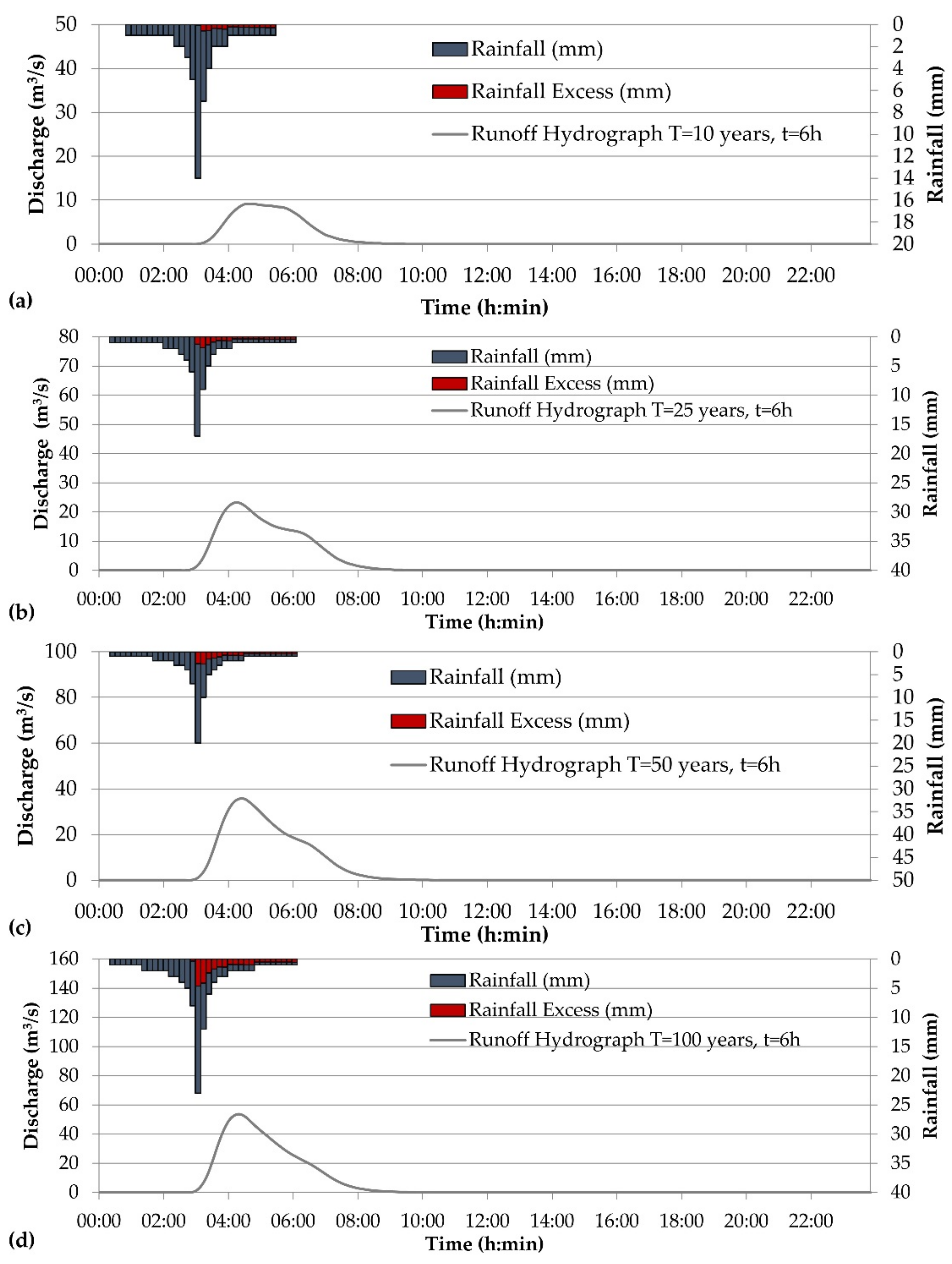
2.2. Hydrologic Simulations and Flood Hazard

Hydrologic simulations were undertaken employing the Hydrologic Modeling System (HEC-HMS) software [32]. HEC-HMS has been developed by the United States Army Corps of Engineers Hydrologic Engineering Center and is designed for the simulation of all hydrological processes. HEC-HMS is used for both event-based and continuous simulation. In the present work, all hydrologic simulations were performed without delineating the Agia Aikaterini catchment into subcatchments. In our hydrologic model, we chose not to delineate our basin, as this would result in lower peak discharges and augmented uncertainty due to the uncertainty involved with the estimation of routing parameters. The following models were selected: (i) the Unitless Soil Conservation Service (SCS) Unit Hydrograph for the transform method, (ii) the SCS Curve Number (CN) method for estimating the rainfall excess, (iii) the Giandotti equation [33,34] for estimating the time of concentration and (iv) the Alternating block method [35] for the rainfall distribution. For better defining the design hyetograph, a stochastic rainfall generator could be possibly introduced in Part 2 of the proposed tool, substituting the Alternating Block Method. The Giandotti equation [33,34] (Equation (2)) was selected as it is the one proposed by the Greek technical specifications for hydraulic works:
t c = 4 A + 1.5 L 0.8 H
where tc is the time of concentration (h), A is the catchment area (km2), L is the length of the main channel (km) and H is the difference between mean altitude and elevation at the outlet of the catchment (m). Based on Equation (2), the time of concentration for the Agia Aikaterini catchment was estimated to be 2.0 h.
The mean CN for the entire catchment was estimated to be 62. CN was estimated based on the 2018 Corine Land Cover map and the soil map of the study area. In the present work, flood depths were estimated based on the results previously reported by Handrinos et al. [36]. In their study, Handrinos et al. [36] employed the widely used HEC-RAS software for simulating flood depths, flow velocities and flood extent of the catastrophic flood event that hit the city of Mandra. They used as input an ensemble of 100 flood hydrographs derived from the simulation of the rainfall–runoff process of the Agia Aikaterini catchment. We utilized these data in estimating flood depths for different return periods (10, 25, 50 and 100 years). Linear interpolation (between maximum peak flow and estimated inundation depth) was undertaken by using the estimated maximum inundation depths at 44 points in the city of Mandra. In addition, the IDW method was used for estimating flood depth in the entire study area. The main assumption of the IDW method is that the attribute value of an unsampled point is the weighted average of known values within the neighborhood, and the weights are inversely related to the distances between the prediction location and the sampled locations [37].
For the hydrologic model, we did not have available rainfall–runoff measurements in this ungauged basin. As a result, it would be impossible to calibrate and validate our model. For the hydraulic model, we used field-measured maximum flood depth marks and the results of a previous study [36], and we exploited the IDW approach in order to minimize the computational resources needed and keep the time needed at reasonable levels. Thus, the hydraulic model was calibrated. Regarding the uncertainty associated with the use of the models, the parameter estimation and the IDW approach, this could be simply resolved by introducing a new part in the proposed tool to perform uncertainty quantification by means of Monte Carlo analysis.

2.3. Flood Risk

Risk can be defined as follows:
R = H V E
where H is the hazard, V is the vulnerability and E is the exposure.
The flood risk of a potential event can be calculated based on the water depths along with estimating the number of objects (e.g., buildings, roads, etc.) affected in the area of interest. Specifically, it can be expressed in monetary units, calculating every component of the risk as follows [38]: (i) hazard, namely, the flood depth expressed in meters, is transformed to the damage percentage of the object, employing a depth–damage curve; (ii) vulnerability is the maximum damage expressed in monetary units, which corresponds to 100% hazard; and (iii) exposure is the number of the inundated objects.
The Joint Research Center (JRC) is the European Commission’s Science and Knowledge Service and has proposed depth–damage functions for every continent and for several classes [9]. According to JRC [9], the available damage functions are categorized into five classes in the form of empirical distribution functions. Figure 3 presents various depth–damage functions used in the present work. All are applicable to residential areas. In addition, we employed six other depth–damage functions, except for the one proposed by JRC. These functions are (i) the Moschato function [5], (ii) the Palermo function [6], (iii) the function reported by USACE [16], (iv) the function reported by FIA [18], (v) the function reported by Appelbaum [15] and (vi) the function reported by Debo [17].
Equation (4) was developed by fitting a non-linear function to the raw data reported by JRC [9]:
D F = ( 1 e x p ( 0.487 h 1.009 ) )
where DF is the estimated damage (%) and h is flood depth (m). The form of the function was based on two main principles. First of all, the function should pass from the point (0, 0), because a flood depth equal to zero should not give damage percentage values other than zero. In addition, the function should have an asymptotic value equal to one, in order to avoid the extrapolation errors, which can be significant in non-linear functions.
Finally, flood risk in monetary terms was estimated based on the maximum depth per building block, the damage percentage per building block estimated employing Equation (3) and a real estate value of EUR 1000 per m2. This cost refers to the current market value of buildings for the study area [39] as reported by the Ministry of Finance of Greece. Finally, it must be mentioned that we assumed that in each building block, residential area (i.e., buildings) accounts for 66%, according to the land use–land cover types of the study area.

3. Results and Discussion

3.1. Hydrologic Simulations
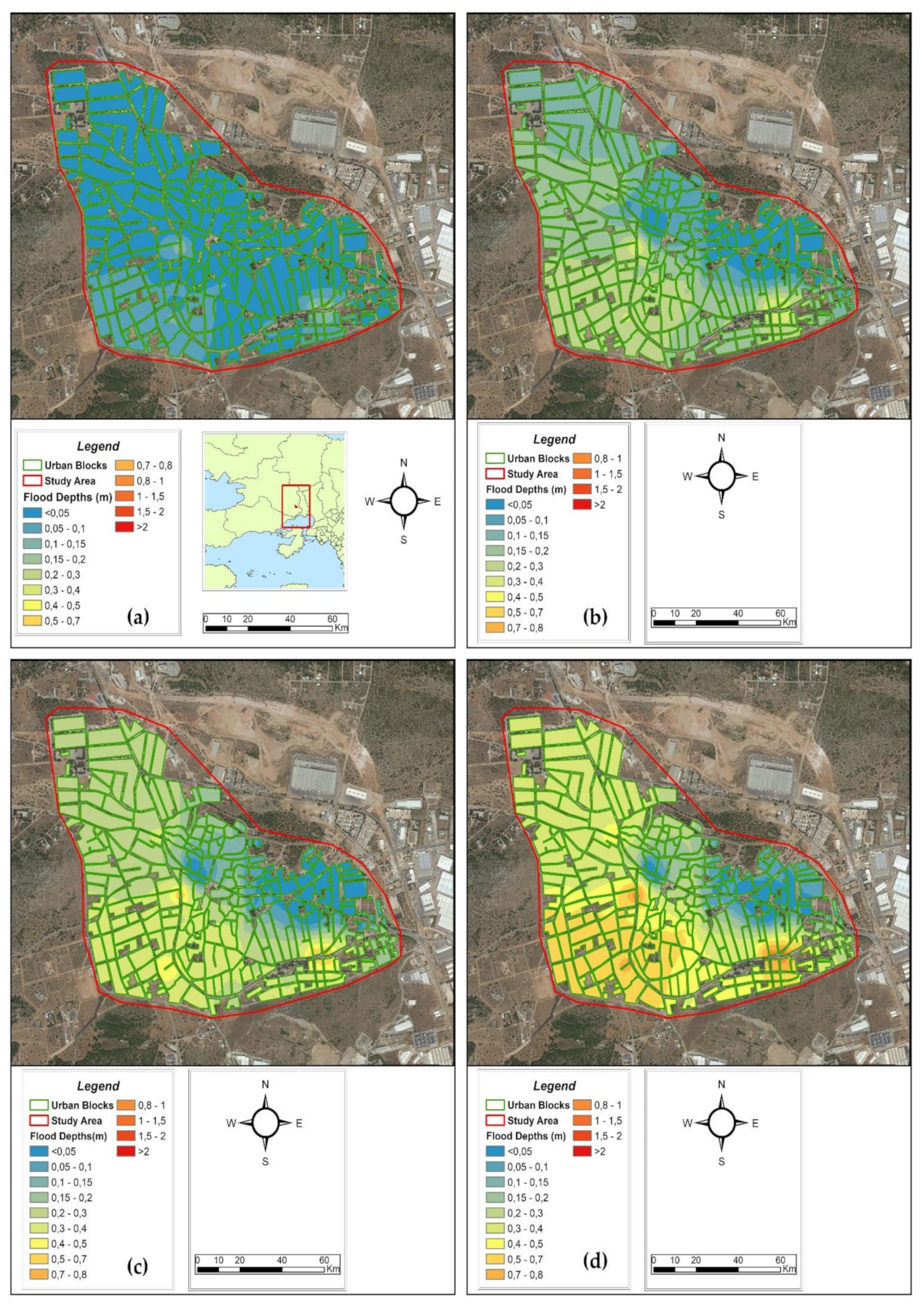
Figure 4 presents the results of the hydrological simulation for rainfall duration of 6 h and return periods of 10, 25, 50 and 100 years. Flood peaks were estimated at about 10 m3/s, 23 m3/s, 36 m3/s and 54 m3/s for return periods of 10, 25, 50 and 100 years, respectively. Total flooding volumes were estimated at 90,300 m3, 228,900 m3, 333,500 m3 and 482,500 m3 for return periods of 10, 25, 50 and 100 years, respectively. It must be stated that we chose not to use probabilities of occurrence lower than 0.01 in order to not introduce extra uncertainty as a result of the extrapolation needed.

3.2. Flood Hazard

Flood hazard was estimated based on linear interpolation and the IDW method, as previously described. Figure 5 presents the estimated results with respect to the flood inundation depths for rainfall duration of 6 h and return periods of 10, 25, 50 and 100 years. For a return period of 10 years, maximum depths ranged from 0.0 to 0.19 m; for a return period of 25 years, maximum depths ranging from about 0.0 m to 0.46 m were estimated. Finally, for return periods of 50 years and 100 years, maximum depths ranged from 0.0 to 0.72 m and 0.0 to 1.08 m, respectively.

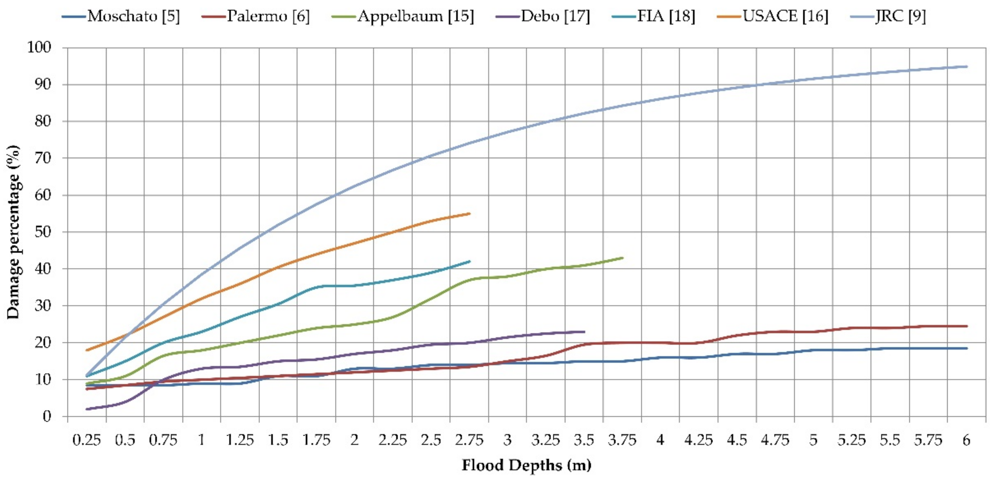
3.3. Flood Risk and Comparison

Figure 6a presents the costs of repairs calculated with the use of Figure 3: (i) the Moschato function [5], (ii) the Palermo function [6], (iii) the function reported by USACE [16], (iv) the function reported by FIA [18], (v) the function reported by Appelbaum [15], (vi) the function reported by Debo [17] and (vii) the function estimated based on the JRC report [9]. Moreover, in Figure 6a the actual cost of repairs for the Mandra catastrophic flood event is presented (red circle). The return period for this event was more than 100 years. This cost was estimated at about EUR 32,000,000 [39]. The aforementioned costs refer to state compensations and compensations from insurance companies. Accordingly, Figure 6b presents the average cost of repairs per building block estimated based on the seven aforementioned depth–damage functions. All costs presented in Figure 6 have been calculated for return periods of 10, 25, 50 and 100 years. Finally, Figure 7 and Figure 8 present the flood risk for return periods of 50 and 100 years, respectively, estimated with the use of all aforementioned depth–damage functions for the study area.
It can be observed that for return periods of 10 and 25 years, the calculated cost for all methods except for the JRC function are of the same order of magnitude and are ranging between EUR 10,000,000 and 90,000,000. The main reason for this is that these relationships were derived as ad hoc functions developed based on a limited amount of flood data, and therefore, it is difficult to generalize them at low water depths.
Moreover, for return periods of 50 and 100 years, the total cost ranges from about EUR 16,000,000 to 95,000,000 and from about EUR 20,000,000 to about 108,000,000, respectively. It can be observed (Figure 6, Figure 7 and Figure 8) that the depth–damage curves of JRC [9], USACE [16], FIA [18] and Appelbaum [15] overestimate the cost compared to the curves for Moschato [5], Palermo [6] and the one proposed by Debo [17]. The main reason is associated with the sparse urban sprawl in the USA in contrast to the dense urban sprawl in Europe, and especially in the Mediterranean region. The functions for Palermo and Moschato give comparable results as they refer to sites with similar characteristics, e.g., climatological, flood regime, land use–land cover type, population and development density, construction materials, etc. In addition, these differences are related to the empirical nature of these curves. The curves for Moschato and Palermo were developed after flood events in the Mediterranean region, while the depth–damage curves of Debo [17] are synthetic curves developed after an economic model was applied on damage results in Georgia, USA. Moreover, the curves of USACE [16], FIA [18] and Appelbaum [15] were developed based on ex post flood damages reported for different regions in the USA. As a result, differences were expected as site characteristics, housing and development type, cost of repairs and materials, among other factors, refer to USA conditions and prices. Regarding the JRC methodology, it seems that it gives the biggest risk in monetary terms, and is comparable to that estimated by the USACE method.
Overall, it can be concluded that the depth–damage functions reported by Pistrika et al. (Moshato curve [5]) and Oliveri and Santoro (Palermo curve [6]) are closer to the real damage cost for Mandra city. However, our intention is not to promote one or another function, but to demonstrate the uncertainties associated with this issue. It must be mentioned that the assessment of flood risk based on empirical depth–damage curves is a subject not well-addressed in the literature. Therefore, it constitutes a very interesting subject from both a practical and future research perspective.
Moreover, it must be mentioned that the use of new low-cost technologies, open data and participatory methods for data collection to provide the necessary geospatial infrastructure either from an office (no field measurements) or combined with field work by volunteers can effectively support the proposed tool for residential flood risk assessment and post-disaster recovery. The tool could be particularly valuable for flood risk assessment in informal settlements, where there is usually a lack of geospatial infrastructure and/or rainfall–runoff measured data. For this application, most of the needed data in Greece can be provided by existing geospatial infrastructure and open datasets for free (e.g., Corine Land Cover, Hellenic Cadastre, Ministry of Government and Energy). Trained volunteers may collect all needed data remotely. These crowdsourced data, following a professional validation, may contribute to building the needed geospatial information for hydrological applications and for planning for emerging demands from a distance (remotely) in a Fit-For-Purpose (FFP) manner, being timely, affordable and reliable.
A possible next step of this research may be the modeling of a crowdsourced methodology for an FFP geospatial data collection that could be used for flood risk assessment in informal settlements. The proposed methodology should focus on the following steps: (i) investigation of the required accuracies of the geospatial data to be used for specific hydrological applications, (ii) investigation of the appropriate tools and methods of collecting all the needed information, (iii) selection and training of volunteers for crowdsourcing, (iv) validation of the crowdsourced data, (v) editing of the geospatial information by a professional engineer and (vi) evaluation of the proposed tool in terms of geometric accuracy and completeness.

4. Conclusions

A robust and fast data-driven tool for residential flood risk assessment is presented here. In addition, an equation fitted through the depth–damage points proposed by the Joint Research Center (JRC) was introduced. The proposed tool incorporates seven different depth–damage functions and is based on free software; thus, it can be applied in different parts of the world and is relatively easy to modify. The proposed tool is based on hydrological simulations employing a free and widely used tool, estimation of flood depths employing linear interpolation and the Inverse Distance Weighting interpolation method in previously reported flood depths, and finally, estimating flood risk, in monetary terms, using seven different depth–damage functions. The tool was tested in an urban area in Mandra, Attica region, Greece, recently affected by a catastrophic flood event. In addition, the results of seven depth–damage functions in terms of estimated monetary cost for the study area were compared. The comparison with previous studies [4,19], which applied the same depth–damage functions, revealed that the results are comparable. However, the current results were not compared with those reported by other researchers, as the results revealed that the depth–damage functions developed from ex post flood damages in the Mediterranean region are more appropriate for this region compared to the costs estimated from depth–damage functions developed for the USA. Moreover, the wide range of the costs is indicative of the high level of uncertainty in this kind of analysis (e.g., aleatory and epistemic). The proposed tool can be possibly used by scientists and engineers, practitioners and/or stakeholders as a first step for better understanding and quantifying flood risk in monetary terms. The proposed fast data-driven tool for the assessment of flood risk in monetary terms can be extended in order to incorporate a stochastic rainfall generator [40,41,42,43,44]. The weather generator is to be used instead of the Alternating Block Method for better defining the design hyetograph. Finally, the proposed tool can be extended by introducing a new part that could account for epistemic uncertainty.

Author Contributions

Conceptualization, Z.T., I.M.K., C.P. and V.A.T.; methodology, I.M.K., V.B. and V.A.T.; software, Z.T. and I.M.K.; validation, I.M.K., V.B., K.A., C.P. and V.A.T.; formal analysis, Z.T., I.M.K. and V.B.; investigation, Z.T.; resources, I.M.K.,V.B., C.P., and V.A.T.; data curation, Z.T., I.M.K. and V.B.; writing—original draft preparation, Z.T. and I.M.K.; writing—review and editing, I.M.K., V.B., K.A., C.P. and V.A.T.; visualization, Z.T., I.M.K. and V.B.; supervision, C.P. and V.A.T. All authors have read and agreed to the published version of the manuscript.

Funding

This research received no external funding.

Institutional Review Board Statement

Not applicable.

Informed Consent Statement

Not applicable.

Data Availability Statement

The datasets generated and/or analyzed during the current study are available from the corresponding author upon reasonable request.

Acknowledgments

The authors would like to thank all the anonymous reviewers whose comments have greatly improved this manuscript.

Conflicts of Interest

The authors declare no conflict of interest.

References

  1. Diakakis, M.; Mavroulis, S.D.; Deligiannakis, G. Floods in Greece, a statistical and spatial approach. Nat. Hazards 2012, 62, 485–500. [Google Scholar] [CrossRef]
  2. Emergency Disaster Database (EM-DAT). Available online: https://apdim.unescap.org/knowledge-hub/emergency-events-database-em-dat (accessed on 5 July 2022).
  3. Apostolopoulos, K.; Potsiou, C. Consideration on how to introduce gamification tools to enhance citizen engagement in crowdsourced cadastral surveys. Surv. Rev. 2021, 54, 142–152. [Google Scholar] [CrossRef]
  4. Kourtis, I.M.; Bellos, V.; Kopsiaftis, G.; Psiloglou, B.; Tsihrintzis, V.A. Methodology for holistic assessment of grey-green flood mitigation measures for climate change adaptation in urban basins. J. Hydrol. 2021, 603, 126885. [Google Scholar] [CrossRef]
  5. Pistrika, A.; Tsakiris, G.; Nalbantis, I. Flood Depth-Damage Functions for Built Environment. Environ. Process. 2014, 1, 553–572. [Google Scholar] [CrossRef]
  6. Oliveri, E.; Santoro, M. Estimation of urban structural flood damages: The case study of Palermo. Urban Water 2000, 2, 223–234. [Google Scholar] [CrossRef]
  7. De Moel, H.; Jongman, B.; Kreibich, H.; Merz, B.; Penning-Rowsell, E.; Ward, P. Flood risk assessments at different spatial scales. Mitig. Adapt. Strateg. Glob. Chang. 2015, 20, 865–890. [Google Scholar] [CrossRef]
  8. Nguyen, V.D.; Metin, A.D.; Alfieri, L.; Vorogushyn, S.; Merz, B. Biases in national and continental flood risk assessments by ignoring spatial dependence. Sci. Rep. 2020, 10, 19387. [Google Scholar] [CrossRef]
  9. Huizinga, J.; de Moel, H.; Szewczyk, W. Global Flood Depth-Damage Functions: Methodology and the Database with Guidelines; JRC Research Reports; Joint Research Centre: Sevilla, Spain, 2017; Available online: https://ec.europa.eu/jrc10.2760/16510 (accessed on 5 July 2022).
  10. Tsakiris, G.; Nalbantis, I.; Pistrika, A. Critical Technical Issues on the EU Flood Directive. Eur. Water 2009, 25, 39–51. [Google Scholar]
  11. European Council. Directive (2007/60/EU) of the European Parliament and of the European Council on the Estimation and Management of Flood Risks. 2007. Available online: http://eur-lex.europa.eu/legal-content/EN/TXT/?uri=CELEX:32007L0060 (accessed on 5 July 2022).
  12. Nalbantis, I. Use of multiple-time-step information in rainfall-runoff modeling. J. Hydrol. 1995, 65, 135–139. [Google Scholar] [CrossRef]
  13. Nalbantis, I.; Lymperopoulos, S. Assessment of flood frequency after forest fires in small ungauged basins based on uncertain measurements. Hydrol. Sci. J. 2012, 57, 52–72. [Google Scholar] [CrossRef]
  14. Batelis, S.C.; Nalbantis, I. Potential effects of forest fires on streamflow in the Enipeas river basin, Thessaly, Greece. Environ. Process. 2014, 1, 73–85. [Google Scholar] [CrossRef]
  15. Appelbaum, S.J. Determination of urban flood damage. J. Water Resour. Plan. Manag. 1985, 111, 269–283. [Google Scholar] [CrossRef]
  16. USACE. Generic Depth-Damage Relationships; United States Army Corps of Engineers: New Orleans, LA, USA, 2000.
  17. Debo, T.N. Urban flood damage estimation curves. J. Hydraul. Div. 1982, 108, 1059–1069. [Google Scholar] [CrossRef]
  18. FIA. Depth-Percent Damage Curves; Federal Insurance Administration, US Department of Housing and Urban Development: Washington, DC, USA, 1974.
  19. Kourtis, I.M.; Tsihrintzis, V.A.; Baltas, E. A robust approach for comparing conventional and sustainable flood mitigation measures in urban basins. J. Environ. Manag. 2020, 269, 110822. [Google Scholar] [CrossRef]
  20. Kourtis, I.M.; Tsihrintzis, V.A. Economic valuation of ecosystem services provided by the restoration of an irrigation canal to a riparian corridor. Environ. Process. 2017, 4, 749–769. [Google Scholar] [CrossRef]
  21. Bellos, V.; Papageorgaki, I.; Kourtis, I.; Vangelis, H.; Kalogiros, I.; Tsakiris, G. Reconstruction of a flash flood event using a 2D hydrodynamic model under spatial and temporal variability of storm. Nat. Hazards 2020, 101, 711–726. [Google Scholar] [CrossRef]
  22. Noto, L.V.; La Loggia, G. Use of L-moments approach for regional flood frequency analysis in Sicily, Italy. Water Resour. Manag. 2008, 23, 2207–2229. [Google Scholar] [CrossRef]
  23. Eregno, F.E.; Nilsen, V.; Seidu, R.; Heistad, A. Evaluating the trend and extreme values of faecal indicator organisms in a raw water source: A potential approach for watershed management and optimizing water treatment practice. Environ. Process. 2014, 1, 287–309. [Google Scholar] [CrossRef]
  24. Tsakiris, G.; Kordalis, N.; Tsakiris, V. Flood double frequency analysis: 2D-Archimedean copulas vs. bivariate probability distributions. Environ. Process. 2015, 2, 705–716. [Google Scholar] [CrossRef]
  25. Yannopoulos, S.; Eleftheriadou, E.; Mpouri, S.; Giannopoulou, I. Implementing the requirements of the european flood directive: The case of ungauged and poorly gauged watersheds. Environ. Process. 2015, 2, 191–207. [Google Scholar] [CrossRef]
  26. Razmi, A.; Golian, S.; Zahmatkesh, Z. Non-stationary frequency analysis of extreme water level: Application of annual maximum series and peak-over threshold approaches. Water Resour. Manag. 2017, 31, 2065–2083. [Google Scholar] [CrossRef]
  27. Stojkovic, M.; Simonovic, S.P. Mixed General extreme value distribution for estimation of future precipitation quantiles using a weighted ensemble—Case study of the Lim River Basin (Serbia). Water Resour. Manag. 2019, 33, 2885–2906. [Google Scholar] [CrossRef]
  28. Ullah, H.; Akbar, M. Drought risk analysis for water assessment at gauged and ungauged sites in the low rainfall regions of Pakistan. Environ. Process. 2021, 8, 139–162. [Google Scholar] [CrossRef]
  29. Razmi, A.; Mardani-Fard, H.A.; Golian, S.; Zahmatkesh, Z. Time-varying univariate and bivariate frequency analysis of nonstationary extreme sea level for New York City. Environ. Process. 2022, 9, 8. [Google Scholar] [CrossRef]
  30. Tegos, A.; Ziogas, A.; Bellos, V.; Tzimas, A. Forensic hydrology: A complete reconstruction of an extreme flood event in data-scarce area. Hydrology 2022, 9, 93. [Google Scholar] [CrossRef]
  31. Flood Risk Management Plan for Attica River Basin District (EL06) (2017) IDF Curves. Available online: https://floods.ypeka.gr/egyFloods/gr06/report/I_1_P02_EL06.pdf (accessed on 5 July 2022). (In Greek).
  32. Zotou, I.; Bellos, V.; Gkouma, A.; Karathanassi, V.; Tsihrintzis, V.A. Using Sentinel-1 imagery to assess predictive performance of a hydraulic model. Water Resour. Manag. 2020, 34, 4415–4430. [Google Scholar] [CrossRef]
  33. Giandotti, M. Previsione Delle Piene e Delle, Magre dei Corsi D’acqua; Istituto Poligrafico dello Stato: Rome, Italy, 1934; pp. 107–117. [Google Scholar]
  34. Mimikou, M.A.; Baltas, E.A.; Tsihrintzis, V.A. Hydrology and Water Resource Systems Analysis; CRC Press: Boca Raton, FL, USA, 2016. [Google Scholar]
  35. Chow, V.; Maidment, D.; Mays, L. Applied Hydrology; McGraw-Hill Book Company: New York, NY, USA, 1988. [Google Scholar]
  36. Handrinos, S.; Bellos, V.; Sibetheros, I.A. Simulation of an urban flash flood: The 2017 flood event in Mandra, Attica. In Proceedings of the 17th International Conference on Environmental Science & Technology, Athens, Greece, 1–4 September 2021. [Google Scholar]
  37. Lu, G.; Wong, D. An adaptive inverse distance weightinh spatial interpolation technique. Comput. Geosci. 2008, 34, 1044–1055. [Google Scholar] [CrossRef]
  38. Jonkman, N.S.; Bočkarjovab, M.; Kokc, M.; Bernardinid, P. Integrated hydrodynamic and economic modelling of flood damage in the Netherlands. Ecol. Econ. 2008, 66, 77–90. [Google Scholar] [CrossRef]
  39. Price Zones of Objective Determination of Real Estate Values. Available online: https://www.gov.gr/upourgeia/upourgeio-oikonomikon/oikonomikon/antikeimenikos-prosdiorismos-axion-akineton-apaa (accessed on 5 July 2022).
  40. Kim, D.; Onof, C. A stochastic rainfall model that can reproduce important rainfall properties across the timescales from several minutes to a decade. J. Hydrol. 2020, 589, 125150. [Google Scholar] [CrossRef]
  41. Paschalis, A.; Molnar, P.; Fatichi, S.; Burlando, P. On temporal stochastic modeling of precipitation, nesting models across scales. Adv. Water Resour. 2014, 63, 152–166. [Google Scholar] [CrossRef]
  42. De Luca, D.L.; Petroselli, A. STORAGE (STOchastic RAinfall generator): A user-friendly software for generating long and high-resolution rainfall time series. Hydrology 2021, 8, 76. [Google Scholar] [CrossRef]
  43. Wheater, H.S.; Chandler, R.E.; Onof, C.J.; Isham, V.S.; Bellone, E.; Yang, C.; Lekkas, D.; Lourmas, G.; Segond, M.L. Spatial-temporal rainfall modelling for flood risk estimation. Stoch. Environ. Res. Risk Assess. 2005, 19, 403–416. [Google Scholar] [CrossRef]
  44. Cowpertwait, P.S.P. Further developments of the Neyman-Scott clustered point process for modeling rainfall. Water Resour. Res. 1991, 27, 1431–1438. [Google Scholar] [CrossRef]
Figure 1. Flow chart of the proposed data-driven tool for flood risk assessment.
Hydrology 09 00147 g001
Figure 2. (a) Location of study area and land uses; (b) residential blocks in the study area and city boundary; (c) Agia Aikaterini catchment upstream of the study area and digital elevation model.
Hydrology 09 00147 g002
Figure 3. Depth–damage function for residential class [5,6,9,15,16,17,18].
Hydrology 09 00147 g003
Figure 4. Hydrologic simulations for rainfall duration of 6 h and return periods of (a) 10 years, (b) 25 years, (c) 50 years and (d) 100 years.
Hydrology 09 00147 g004
Figure 5. Flood inundation depths for rainfall duration of 6 h and return periods of (a) 10 years, (b) 25 years, (c) 50 year and (d) 100 years.
Hydrology 09 00147 g005
Figure 6. (a) Total cost of repairs calculated with various depth–damage functions and for various return periods [5,6,9,15,16,17,18]; (b) average cost of repairs per building block calculated with various depth–damage functions and for various return periods [5,6,9,15,16,17,18].
Hydrology 09 00147 g006
Figure 7. Flood risk, in monetary terms, estimated for the 50-year flood with the various depth–damage functions of (a) Moschato [5], (b) Palermo [6], (c) USACE [16], (d) FIA [18], (e) Appelbaum [15], (f) Debo [17] and (g) JRC [9].
Hydrology 09 00147 g007
Figure 8. Flood risk, in monetary terms, estimated for the 100-year flood with the various depth–damage functions of (a) Moschato [5], (b) Palermo [6], (c) USACE [16], (d) FIA [18], (e) Appelbaum [15], (f) Debo [17] and (g) JRC [9].
Hydrology 09 00147 g008
Table 1. Rainfall depth (mm) for return periods ranging from 2 to 100 years and rainfall durations ranging from 1 to 24 h.
Rainfall Depth (mm) for Various Return Periods (Years)
Duration (h)25102550100
1223137465362
2304150627283
3354959738598
646647796112129
126084101126146168
2478109132164191219
Publisher’s Note: MDPI stays neutral with regard to jurisdictional claims in published maps and institutional affiliations.

