Article

Streamflow Analysis in Data-Scarce Kabompo River Basin, Southern Africa, for the Potential of Small Hydropower Projects under Changing Climate

Department of Civil Engineering, Central University of Technology, Bloemfontein 9300, South Africa
*
Author to whom correspondence should be addressed.
Hydrology 2022, 9(8), 149; https://doi.org/10.3390/hydrology9080149
Submission received: 8 July 2022 / Revised: 8 August 2022 / Accepted: 13 August 2022 / Published: 18 August 2022

Abstract

:
In developing countries with data scarcity challenges, an integrated approach is required to enhance the estimation of streamflow variability for the design of water supply systems, hydropower generation, environmental flows, water allocation and pollution studies. The Flow Duration Curve (FDC) was adopted as a tool that is influenced by topography, land use land cover, discharge and climate change. The data from Global Climate Model (GCM) projections, based on Representative Concentration Pathways (RCP) 4.5 and RCP 8.5 climate scenarios, were used as input data for the SWAT model for the simulation of streamflow. The FDCs were then derived from the simulated streamflow. The FDC for RCP 4.5 showed insignificant differences, whilst for RCP 8.5 it showed an increase of 5–10% in FDC from the baseline period, which is likely to increase the hydropower generation potential with some considerable streamflow variability. The integrated approach of utilizing FDC, GIS and SWAT for the estimation of flow variability and hydropower generation potential could be useful in data scarce regions.

1. Introduction

Hydropower generation is highly recommended in rural communities, especially for developing countries where electricity is a huge challenge. In addition, hydropower generation is a cleaner technology, with minimal negative impact on the environment [1,2]. Hydropower is a more rigorous type of energy than wind and solar energy. Due to the density and kinetic energy of water, the available power is easily estimated, the energy is usually provided on demand, there is no use of fuels, there is minimal maintenance of infrastructure and there is a relatively long-life span of mostly more than 50 years [3,4,5,6]. In this paper, small hydropower generation is considered to be less than 10 MW [7]. Southern Africa, like many other developing regions, experiences data scarcity, making research, assessments and planning difficult. The data scarcity challenges have also been acerbated by climate change effects precipitated by anthropogenic and natural activities [8,9]. This has resulted in further uncertainty in hydropower assessments in the region. Special techniques and methodologies must be devised for the assessment of water resources’ variability across the basin to enhance the estimation of hydropower generation potential and other needs.
The assessment of hydropower potential in an ungauged catchment under climate change and in data scarce regions is an area of active research. Several studies have addressed the assessment of mega-hydropower potential for river basins. For instance, it was reported that Southern Africa could experience major hydrological changes in the coming decades, bringing drastic changes to hydropower. The study focused on four large hydropower dams in the Kafue River and Zambezi River basins, accounting for over 90% of the installed capacity in the basin [10]. It was analyzed that the small hydropower production system of the Southern African region is likely to be strongly affected by changes in climate [11]. A novelty was introduced in the field by advancing the representation of reservoir hydropower generation in energy system modeling by explicitly including the most relevant hydrological constraints in the Zambezi River basin [12]. It was concluded that climate and other risks associated with current and future hydroelectric power generation include projected droughts leading to reduced runoff and reservoir storage capacity that will adversely reduce the power generating capacity [13]. However, none of these studies have analyzed the potential of small hydropower systems in ungauged catchments under the climate change scenario.
In view of the gap identified, the study sought to evaluate streamflow under the changing climate for ungauged catchment using the Flow Duration Curve defined as a cumulative frequency curve that shows the percent of time the specified discharges were equaled or exceeded during a given period [14]. When the FDC is derived from the long-term flows of a stream, it can be used to predict the distribution of future flows for water supply, hydropower generation potential, environmental flows and pollution studies [14].
The methods widely used in the estimation of hydro power generation are non-sequential or the Flow Duration Curve (FDC) and Sequential Stream Routing (SSR) [5,6,15]. The FDC method is recommended for preliminary studies and for high-head run-of-river projects, where head is pre-set, and low-head projects, where head varies with discharge. The SSR is suitable for multipurpose storage projects and for analyzing the feasibility of power at an identified water conservation site or flood control project [15].
The derivation of an accurate FDC largely depends on the availability of quality long-term streamflow data with high resolution. The FDC is a function of biophysical data, such as topography, land use/land cover, soils, precipitation, temperature and discharge [3,16]. Many river basins in the Southern African region are challenged with hydrometeorological data availability and, in some cases, are completely ungauged [17,18,19]. Furthermore, the region has not been spared the effects of climate change, which has a direct influence on the FDC. Many studies have relied on the use of the FDC to estimate hydropower generation potential and the design of water supply schemes as a convention where required data are available [20,21,22,23,24]. However, in cases where the required data are scarce under a changing climate, it becomes vital to find other useful alternatives for derivation of the FDC for the recent past and the future period. In addition, techniques should be developed to help estimate the river potential for reliable water supply and hydropower generation potential in ungauged catchments of the region.
In this paper, an integrated approach was used for the derivation of FDCs from three climate change scenarios that include the historical period of 1975–2005 and RCP 4.5 and RCP 8.5 for the future period of 2020–2050 to determine the hydropower potential variability in response to the changing climate in the data scarce region of the Kabompo River Basin. A methodological approach integrating the regional FDC, linear regression and GIS to estimate flows and potential head for the design of the hydropower for the ungauged sites was used and the results obtained are promising for data scarce regions of Southern Africa. The methodological approach is considered to be a novelty in the Kabompo River Basin and could be useful in developing countries with data scarcity challenges.

2. Materials and Methods
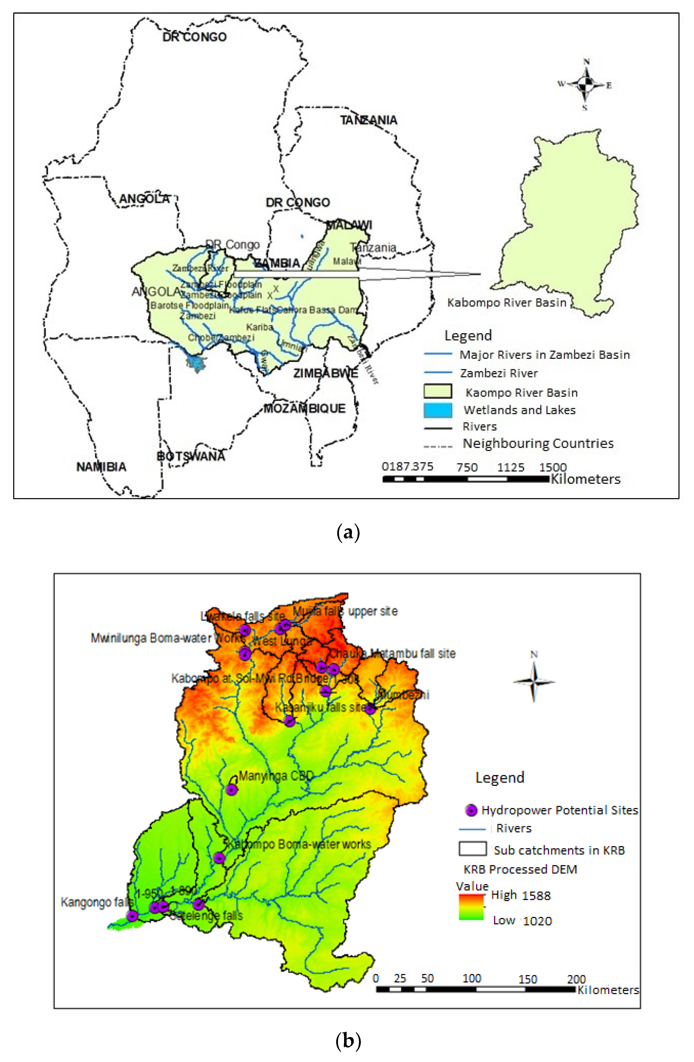
2.1. The Study Site

The Kabompo River Basin (KRB) is part of the Upper Zambezi River Basin in the Southern African region. The KRB originates from the Zambezi–Congo watershed in Mwinilunga district in the north-western part of Zambia. The basin is located within the political boundaries of seven rural districts including Mwinilunga, Solwezi, Kabompo, Zambezi, Mufumbwe, Kasempa and part of Lukulu. Furthermore, the basin has huge potential for hydropower generation, agricultural production, wildlife conservation and mining. Figure 1a,b illustrate the location of the basin with selected gauged and ungauged sites that have a land mass of about 72,087 km2 [25] and Miombo forests as predominant land cover.
The KRB is located just below the equator with a mean annual precipitation of 1200 mm. The basin has a runoff coefficient of not more than 10% on average [26,27]. The basin generates annually about 240 m3/s of runoff on average, significantly contributing to the water resources in the upper ZRB. The time series data for temperatures across the ZRB show variations in accordance with elevation. The hottest month is October, with a mean daily temperature of 29 °C, and the coldest is July, with a mean daily temperature of less than 13 °C. The Potential Evapotranspiration (PET) varies considerably across the basin, from more than 1700 mm per year in the middle ZRB to less than 1400 mm per year in the upper ZRB, and PET in the KRB is estimated to be 1300 mm [26]. The PET in many parts of the ZRB is twice as high as precipitation totals and this affects the overall basin water balance. The Southern African region has been characterized by the effects of climate change with a decadal mean temperature rise in most of the countries, varying from 0.21 °C–0.33 °C in the recent past [28].

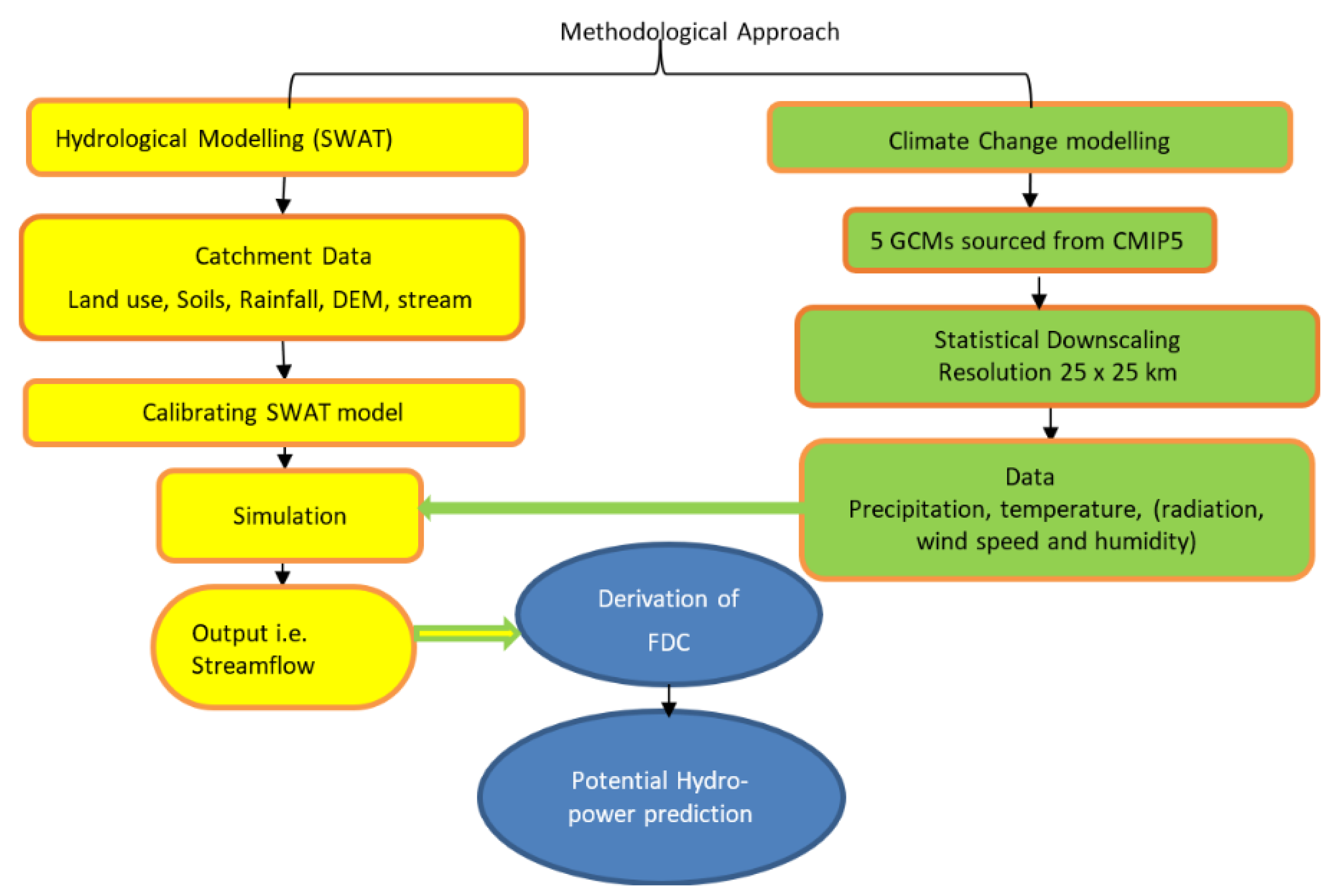
2.2. Methodological Approach

The methodological approach involved hydrological modeling using the Soil Water Assessment Tool (SWAT) model, which was first calibrated and validated using measured catchment data. The calibrated SWAT model was used to simulate streamflow based on five statistically downscaled and bias-corrected GCM data sourced from the Coupled Model Intercomparison Project Phase (CMIP5) for three climate change scenarios. The simulated streamflow was then used for derivation of the FDC, which was the primary tool for the estimation of hydropower potential in the gauged (indexed) sites. The regional FDCs were constructed using regression techniques for the estimation of hydropower potential for the ungauged sites. Figure 2 shows a flow chart of the methodological approach.

2.3. Data for Climate Change Modelling

The five statistically downscaled and bias-corrected GCMs comprised precipitation and maximum and minimum temperatures. The other variables, such as relative humidity, solar radiation and wind speed, were generated based on the historical weather data using a SWAT built-in weather generator [29]. The GCM data set was obtained from NASA Earth Exchange (NEX) Global Daily Downscaled Projections (NEX-GDDP). The climate data set was developed from GCM runs performed by CMIP5 to support the Fifth Assessment Report of the Intergovernmental Panel on Climate Change (IPCC AR5) [30]. The selected GCMs were tested and found out to be in good consensus with sufficient skill. Table 1 shows the GCM used in the study.

2.4. Hydrological Modeling Input Data

The SWAT model input data included soil, land use/land cover, mean monthly rainfall, maximum and minimum temperatures and DEM with a resolution of 30 m. Calibration and validation of the model were performed using observed monthly flow data.
The SWAT model was selected for the simulation of GCM projections sourced from CMIP5 based on the three climate change scenarios. The selection was based on its wide use for climate change impact modeling and on its ability to run a long-term simulation [31]. The model is a continuous, distributed and physically based model that sub-divides the basin into smaller units, known as Hydrologic Response Units (HRU), which are homogenous with similar gradient, land cover and soil properties [15,32]. The SWAT model has proved to be reliable for hydrological modeling in different climates and environments [33].
The calibrated model was forced with five GCM projections based on the baseline period of 1975–2005 and RCP 4.5 and RCP 8.5 for the 2020–2050 period. The RCP4.5 is a middle-pathway scenario that correlates well with the recently released guidelines of lower greenhouse gas emission by the international community. RCP 8.5 is a high-emission scenario, which provides possibly the highest impact on climate change. The two RCPs therefore give a good combination for climate change analysis. The climate variables simulated were precipitation, temperature, wind speed, solar radiation and humidity on a monthly scale; however, in this study, the focus was on precipitation and temperature. The monthly streamflow was simulated for each GCM projection based on the three scenarios and an average ensemble streamflow was created for each climate change scenario.

2.5. Estimation Method for Climate Change Impact

The most commonly used method for change analysis is the change factor methodology (CFM), which is also called the delta change factor method [34,35]. The additive CFM is determined by finding the change of a GCM variable resulting from a recent climate simulation and a future climate scenario based on the identical GCM grid position. The calculated change (delta change) is then added to the measured data to find the simulated future time series. The additive change factors involved the estimation of averages for baseline and future scenarios.

2.6. Methods for Estimation of Hydropower Generation Potential

The primary estimation of hydropower potential is widely done by the Flow Duration Curve (FDC) (non-sequential) and Sequential Streamflow Routing (SSR), which have also been used extensively for water supply, hydropower generation potential and environmental flow estimations [36]. This study focused on the derivation of FDC based on historical and projected discharge. The streamflow is associated with the percentage exceedance values that indicate the percent of time when various levels of streamflow are equaled or exceeded. The FDC can be transformed to a Power Duration Curve (PDC) [24] by using the following Equation (1).
P i = e i γ Q i H i
where P i is the power production (in kW) when the turbine discharge is at exceedance percentage i; e i is the overall plant efficiency with turbine discharge equal to Qi and net head equal to Hi (typically, e is 70–80% for a small scheme); γ is the specific weight of the water (1000 kg/m3 × 9.81 m/s2); Q i is the turbine discharge at percentage exceedance i (Q10, Q20, etc.); turbine discharge is assumed to be equal to the river discharge, except when the river discharge exceeds the turbine capacity or other constraints on the turbine discharge are encountered; H i is the net head available with river flow at exceedance percentage i (Hi is the Net Head (m), i.e., excluding head losses).
The power generated is proportional to the head and the discharge. Overall, the size and cost of the turbine depends on the design flow rather than the hydraulic head [37]. Most of the turbine efficiency for small hydropower schemes are 0.80–0.90 [24]. There are two critical parameters in determining the potential power from a site: the hydraulic head and the flow in the river. However, the flow in the river will tend to vary considerably and quite often on a daily basis. It is of great importance to know what kind of variation there is over a long period (years). These data are often shown in the form of an FDC, a probability model of the frequency that a particular flow rate will occur.
The estimation of the optimum size of a turbine for a site becomes critical. For example, if a bigger turbine is installed, it would give maximum power output at full capacity of power production for only a few days in a given year compared with when a smaller turbine is installed to operate most of the time during a year. However, it does not leverage the larger potential for power generation at higher flows. Therefore, an optimal use must be determined in line with the flow that occurs most of the time during a year to sustain the downstream ecosystem [1,38]

2.7. Procedure for Derivation of Flow Duration Curves

The Flow Duration Curve (FDC) is determined and plotted to analyze streamflow regime and percentage flow exceedances [39,40]. The FDC is important in hydrology as it reveals much of the stream flow’s temporal variability and its shape is a function of different factors [41]. Overall, the whole section of the FDC is analyzed as an indication of groundwater and subsurface flow contribution to streamflow, which is the subsurface catchment storage for a specific catchment [42,43]. The shape of the FDC has continued to be a matter of research because of the many factors that influence it [44]. The procedure for developing the FDC involved arranging the monthly observed flows and the simulated monthly streamflow for KRB in a descending magnitude.

2.8. Estimation of Hydropower Potential for Ungauged Catchment

The flow estimation in ungauged sites has always been a subject of research, as no conventional method with high accuracy has been developed. Many methods have been used with different levels of accuracy [45]. Some of the methods used include the Drainage Area Ratio (DAR), the Standard Mean Method (SMM), the Mean and Standard Deviation Method (MSM) and the Regional Flow Duration Method [45,46,47]. In this study, the Regional Flow Duration Method was used. The method, described by [45,46,47,48], involved the following procedure:
  • Deriving the Flow Duration Curve for all gauged river catchments and standardizing it by dividing the observed Flow Duration Curve by the average of monthly streamflow (the index streamflow) for all the stations with records in the study area.
  • A graphical regional dimensionless Flow Duration Curve is obtained by averaging the standardized observed Flow Duration Curve of all gauged river catchments in the study region. The Flow Duration Curve for ungauged catchments located in the study area was then estimated as the product of the dimensionless regional Flow Duration Curve and an estimated index streamflow for the catchment.

3. Results

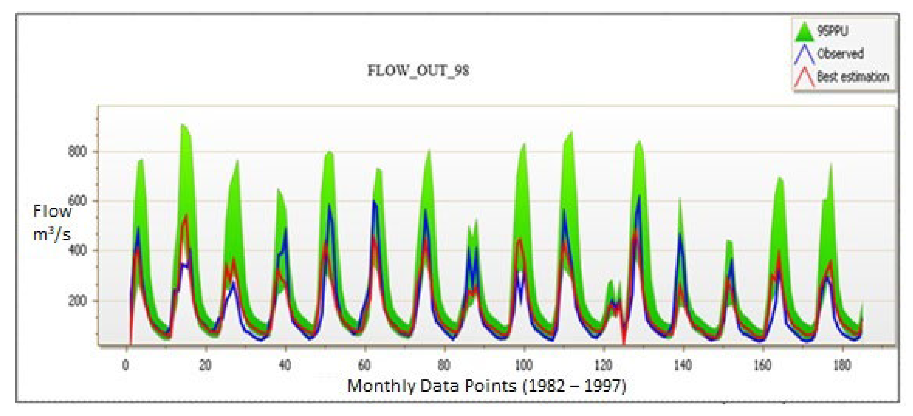
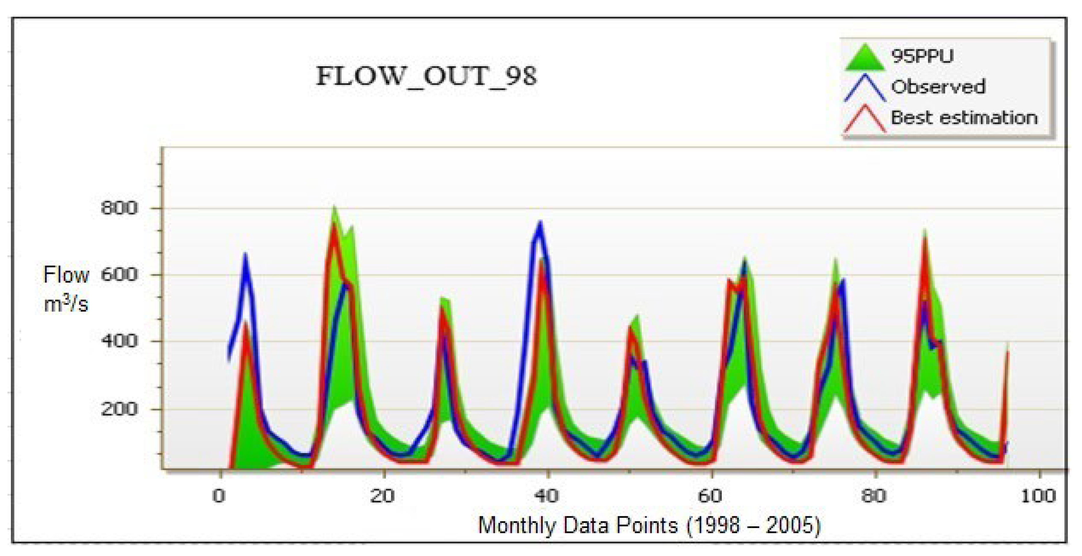
3.1. Calibration and Validation of SWAT Model

The SWAT model simulations were carried out for the period 1979–2013. Model warm up and initialization were done with the first three years of data (1979–1981). Measured streamflow data were obtained from a flow gauge station. Two thirds of the monthly measured flow data from 1982–1997 were used for calibration and the remaining one third of data from 1998–2005 were used for model validation. There were no complete datasets with a high resolution on a daily or hourly basis. For this reason, only monthly measured data were used. The SWAT Calibration and Uncertainty Program (SWAT-CUP) with Sequential Uncertainty Fitting 2 (SUFI-2) were used to evaluate the SWAT model outputs.
The SWAT model was run with 18 input parameters that were subjected to sensitivity analysis. The selected parameters were ranked through the global and local sensitivity analysis [49]. Global sensitivity analysis was evaluated by computation of the multiple regression of the Latin hypercube-produced parameters against the objective function values. The assessment of the sensitivity of parameters in SUFI-2 was measured with the t-stat values and p-values. Table 2 shows the parameters used in the calibration.
The large number of input parameters represented various processes in the objective function of SUFI-2, which improved the enveloping of the observations. The objective functions used were Nash–Sutcliff (NS) and the coefficient of determination (R2) for discharge, while the uncertainty analysis was assessed with the P-factor representing the 95PPU for the model simulation and R-factor, the band representing observed data including its error [49]. The model was successfully calibrated and validated and reached its objective function. Figure 3 Shows the observed and simulated hydrographs of the calibrated model, while Figure 4 shows the observed and simulated hydrographs of the validated SWAT model.
The statistics used to determine the goodness of fit were the Nash–Sutcliffe coefficient (NS) [50] and the coefficient of determination (R2), while the uncertainty analysis was assessed by the P-factor and R-factor. The results are summarized in Table 3.
Table 3 shows a good coefficient of determination (R2) and Nash–Sutcliffe coefficient (NS) for both the calibration and the validation periods in accordance with the recommendation of [32]. The model performance was further evaluated for goodness of fit with the P-factor and the R-factor and Table 3 shows the results to be acceptable in accordance with [49].
The calibrated model was therefore determined to be suitable for the simulation of streamflow for the three climate change scenarios. The simulated streamflow for the KRB was analyzed using the Flow Duration Curve (FDC) that was used to show how it is distributed over a period of 30 years. The FDC shows the relationship between the magnitude of streamflow and its frequency of daily, weekly and monthly streamflow or an interval for a particular river basin [14,36].

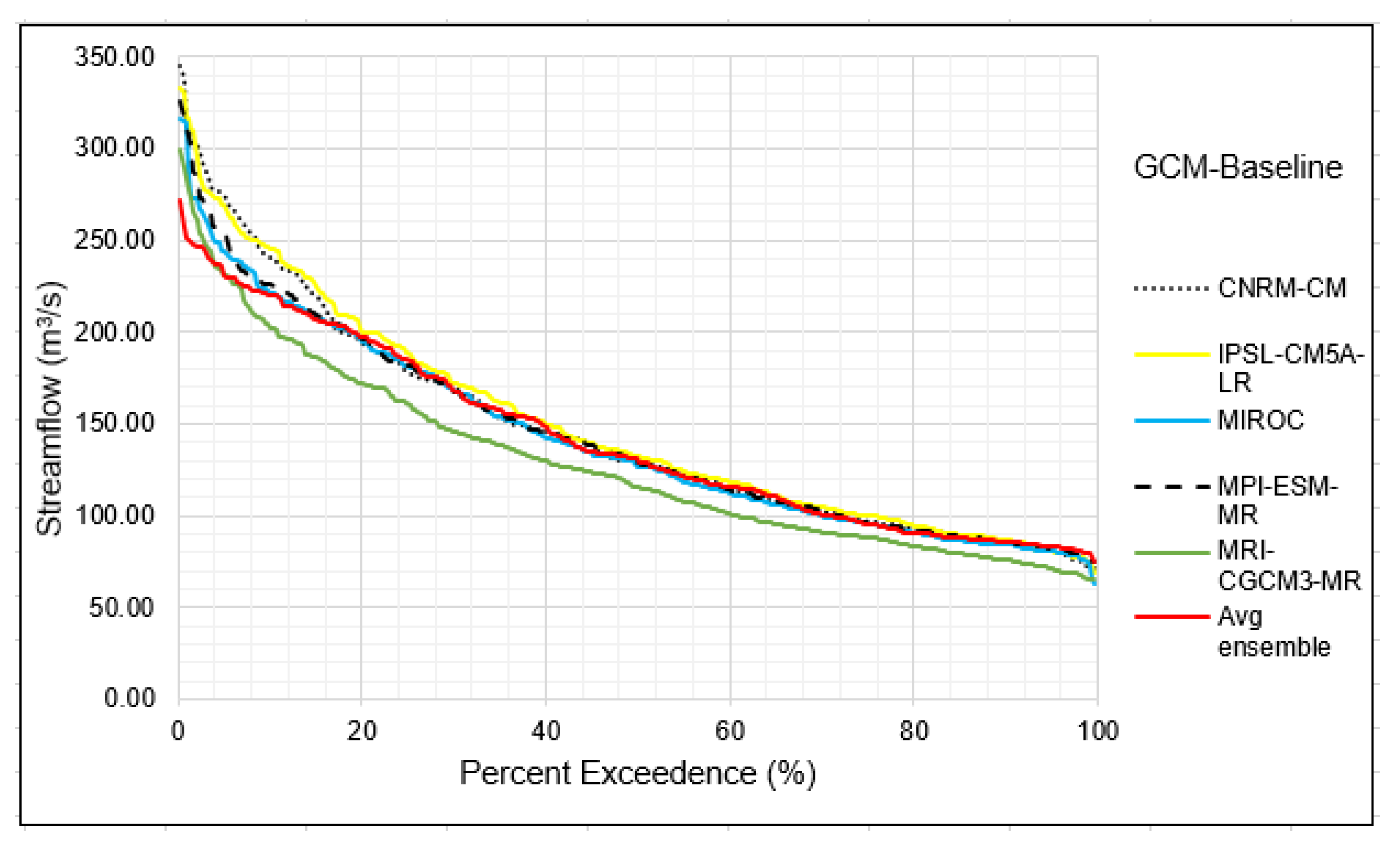
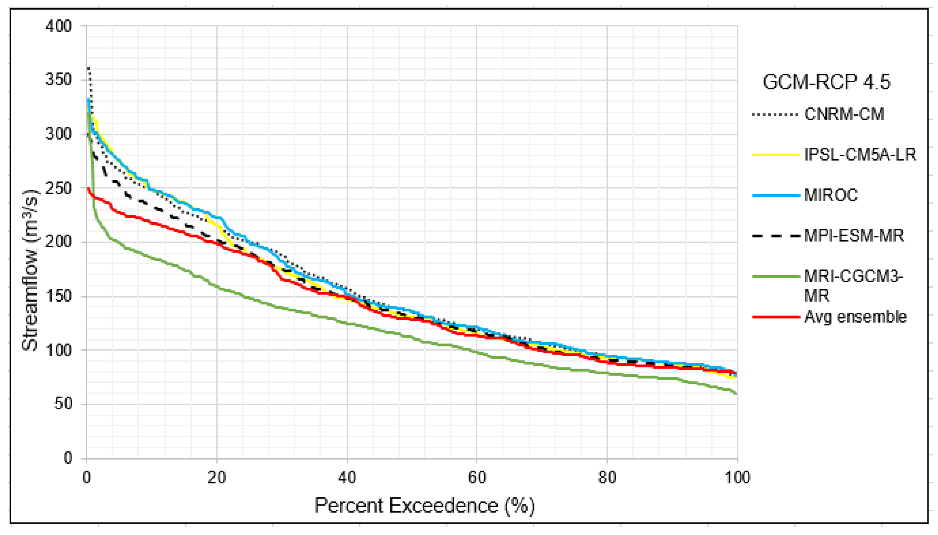
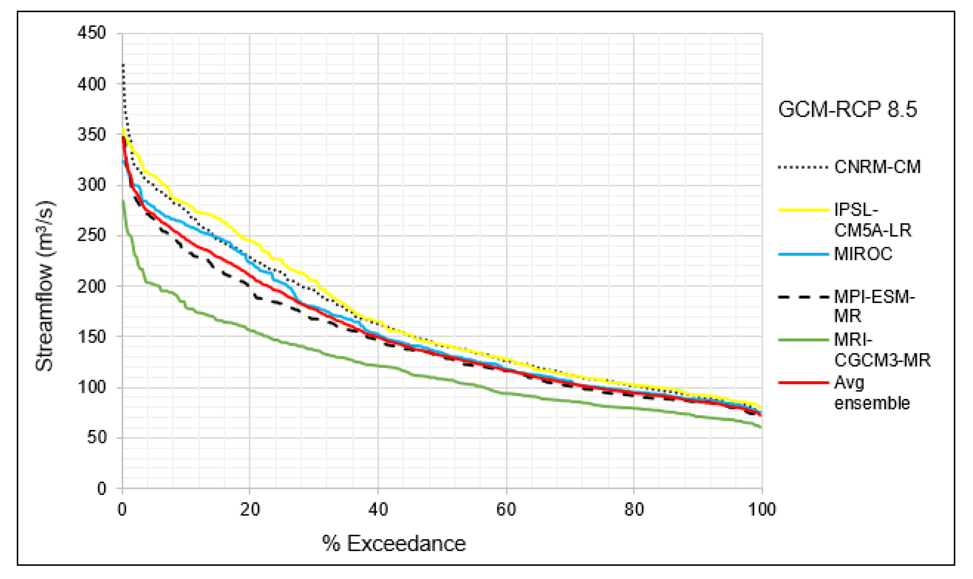
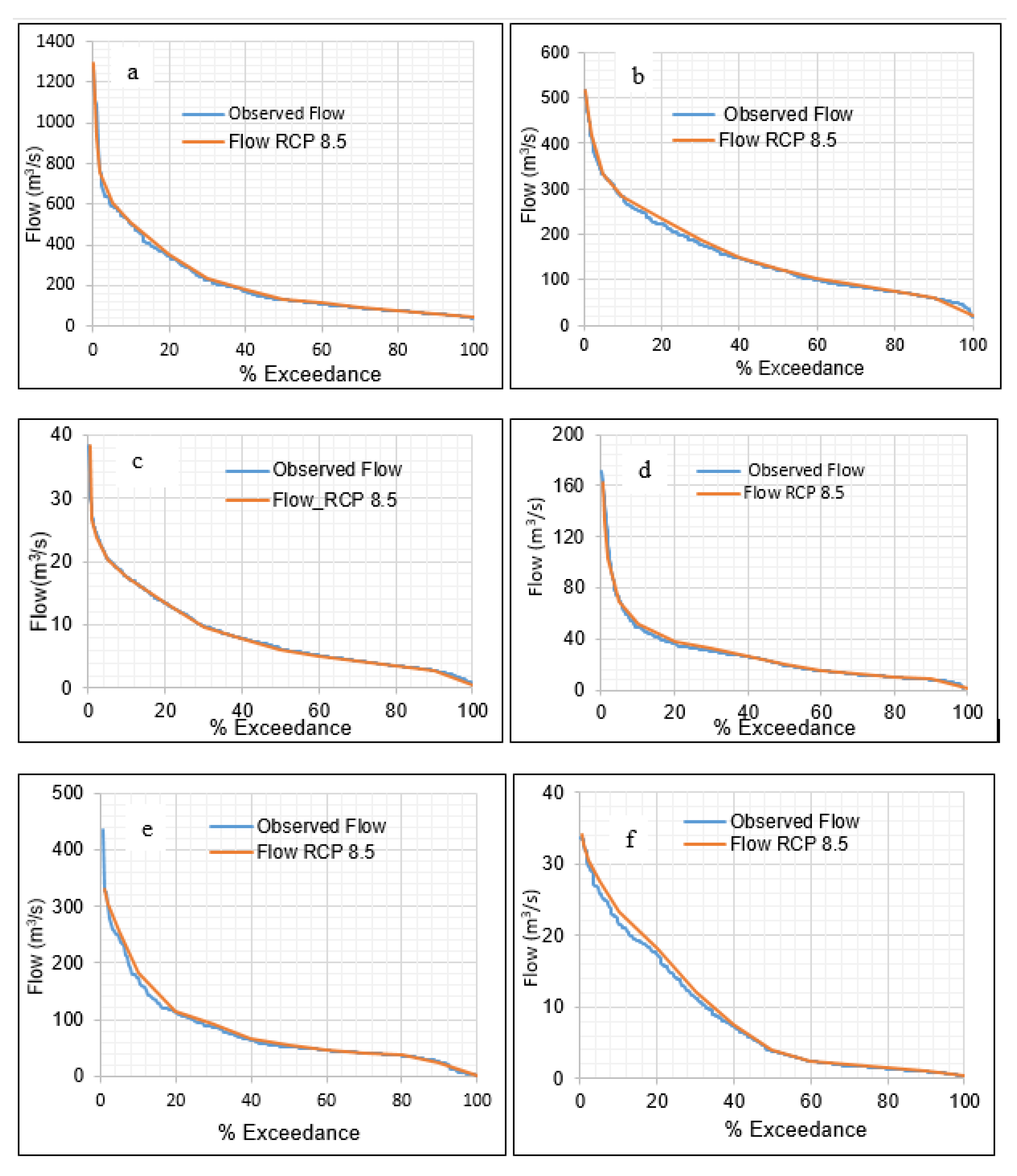
3.2. Derived Flow Duration Curves for GCM

The simulated ensemble monthly streamflow based on five GCMs was analyzed under baseline, RCP 4.5 and RCP 8.5 climate scenarios. The ensemble monthly streamflow [51,52] was analyzed for the FDC in order to determine the basin characteristics under various climate scenarios as projected by the GCMs for easy determination of hydropower potential. Figure 5 indicates the FDCs for all the ensemble streamflow.
Figure 5 shows the FDC for the simulated ensemble streamflow plotted under the baseline period. The variability of the streamflow about the mean is mostly due to the simulations from MRI-CGCM3-MR, which perhaps has unique skill. All the curves exhibit gentle slopes, indicating that the basin has a significant contribution of base flow (spring sources of water) and the capacity to sustain the low flows throughout the year.
The steep slope of the curves for Q10 characterize the flood regime of the basin, which is probably caused by rainfall. However, the high flows, Q10, are characterized by a steep slope, while the low flows, Q70, are characterized by flat curves. The lowest flow that is equaled or exceeded at 100% time (also known as Q100) is 66 m3/s, which is available throughout the year. The flows between Q0 and Q10 are considered as high flows that are only available for a small proportion of time in a year, while flows between Q10 and Q70 are medium-range flows. Flows from Q70–Q100 are the low flows that are available most of the time and are also suitable for hydropower generation. Moving further to the right of the graph, flows from Q95–Q100 are also considered as drought flows. The stream flow variability in Figure 5 influences the estimation of the optimum size of a turbine for a site.
In general, the size and cost of the turbine is a function of the design flow rather than the hydraulic head [37,53]. Q70–Q100 would be suitable flows for the design and estimation of the cost of a turbine for average hydropower generation capacity for all year round. The Q0–Q10 flows would be suitable for the design and estimation of the cost of a turbine for higher hydropower generation capacity only during the peak-flow season. The FDC analysis was extended to a monthly ensemble streamflow under RCP 4.5. The results are shown in Figure 6.
The FDCs in Figure 6 show slopes that are considerably gentle, reflecting the same basin characteristics. There is internal ensemble variability from the mean, which signifies GCM uncertainty. However, the trend shown in Figure 6 is much similar to the baseline scenario described. There was an insignificant impact of climate change under RCP 4.5 on streamflow and, as a result, the FDCs derived were similar to the ones under the baseline period. The RCP 4.5 is a low-emission scenario with restrictions and hence the negligible impact on streamflow. The FDC shows a good consensus except for the FDC that is based on MRI-CGCM3-MR, which varies slightly from the average ensemble, as was the case under the baseline scenario. The high flows are represented by Q0–Q4, where there is a steep slope indicating a flood regime. The flow may only be available for a very short time in the year, reducing the probability of flooding. Flows between Q4 and Q60 are medium range, while low flows occur between Q60 and Q100. In general, the basin will have more low flows under this climate scenario with less likelihood of floods. There is a high probability that low flows may result in drought events.
Further analysis of the FDC for the simulated ensemble was performed under an RCP 8.5 scenario and the results are presented in Figure 7.
Figure 7 shows a simulated ensemble FDC under RCP 8.5, with considerable internal ensemble variability about the mean. There is little consensus between Q0 and Q20. The FDC in Figure 7 shows clear changes in the slope of the FDC with a higher magnitude of the average ensemble FDC. There is a notable impact of climate change on streamflow, which is likely to increase. The RCP 8.5 is a higher-emission scenario (business as usual) and has, therefore, higher projections in climate variables with a potential for considerable impact on streamflow and other hydrological processes. The FDC analyzed from the simulated streamflow can be divided into very steep slope, gentle slope and very flat slope, which is found out to be very different from Figure 5 and Figure 6.
The Q0–Q10 is a very steep slope, indicating the flood regime, which is considered to be a high-flow section. This could last for 10% of the time in a year. The slope indicates the possibility of serious floods, with Q4 flows considered as severe floods. The medium-range flows are between Q10 and Q70, which has a gentler slope, while low flows are between Q70 and Q100, where the slope is very flat. The basin is predicted to experience severe floods under this climate scenario that may require comprehensive preparedness.
The majority of GCMs have shown consensus in that they are generally flat slopes and are not different from the climate scenario under RCP 4.5. There is no likelihood of floods, even for flows between Q0 and Q4.
Further FDC was performed on the simulated ensemble mean streamflow to determine the combined response with a change factor methodology, which is one of the most widely used methods in climate change studies [35]. The calculated delta was added to the observed flows for future time series for RCP 8.5 and RCP 4.5. The results are shown in Figure 8.
The FDC in Figure 8 illustrates the future FDC for RCP 8.5 and RCP 4.5 compared with the observed flows. The figure shows that the future streamflow under RCP 4.5 and 8.5 will not significantly differ from the observed flows. However, there is a variation in flow between Q4 and Q30 for RCP 8.5 and observed flows, which is likely to translate into increased river flows. The positive change in flows under RCP 8.5 may occur only during the rainy season and is likely to increase the potential for hydropower generation in selected sites. The three sections in the FDC are still eminent as very steep, gentler and very flat. There is a very steep slope between Q0 and Q5, with the highest flows in the basin. There is a high probability of severe floods of 600–1300 m3/s, which may occur for about 5% of the time in a year.
The flood regime is most likely to be characterized by high-intensity rainfall. The Q5 to Q20 has a gentle slope with 300–600 m3/s flows, while Q20–Q60 has medium-range flows of 60–300 m3/s. Q60–Q100 is a very flat slope with low flows. The lowest flow is about 40 m3/s at Q100 and is the flow equaled or exceeded throughout the year, which is most reliable for the design of various water uses. The result predicts that, under an RCP 4.5 scenario, the basin will experience similar floods as the baseline period, while for RCP 8.5, there will be a slight increased magnitude of streamflow throughout the year.

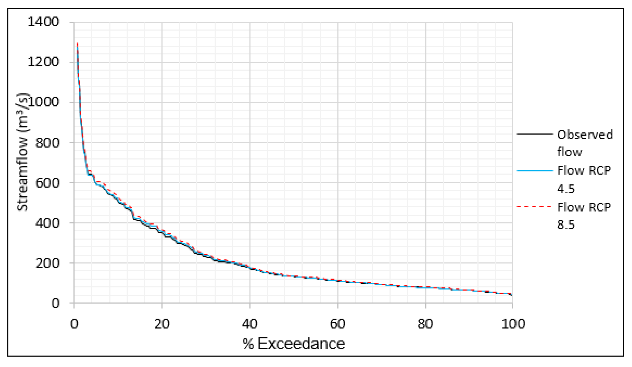
3.3. Derived Flow Duration Curves for Gauged Sites

The basin is characterized by insufficient data with missing values from the available few sites. Complete records only cover specific periods and differ from one station to another. The recorded water levels were converted to an average monthly discharge (m3/s) for each station, using the respective rating equations. The derived FDCs from the observed flow data were compared with the FDCs derived from RCP 8.5, and some variations are clearly noted. Following the procedure described under Section 2.8 of the methodology, the Flow Duration Curves derived for six different sites are illustrated in Figure 9 for the gauged sites in the basin.
The FDCs for Figure 9a,b are constructed from larger drainage areas and hence Q100 flows are also for the same drainage area. Streamflow is likely to increase slightly from Q0–Q40, as illustrated in Figure 10, while Q40–Q100 will remain with minimal difference between observed and RCP 8.5. Figure 9c–f have Q100 flows of less than or equal to 1 m3/s. Q10 represents the quick runoff from precipitation input in all cases, while Q10 to Q60 represent the medium flows and Q60–Q100 are low flows, characterizing baseflow that occurs most of the time in a year. This is also the flow that occurs most of the time in a year and is sometimes referred to as Q95, which is recommended for the design of hydropower generation. The shape of all the FDCs for the basin confirms that the sub-catchments have similar physiographical properties and they are, therefore, suitable for flow transfer to ungauged sites within the basin.

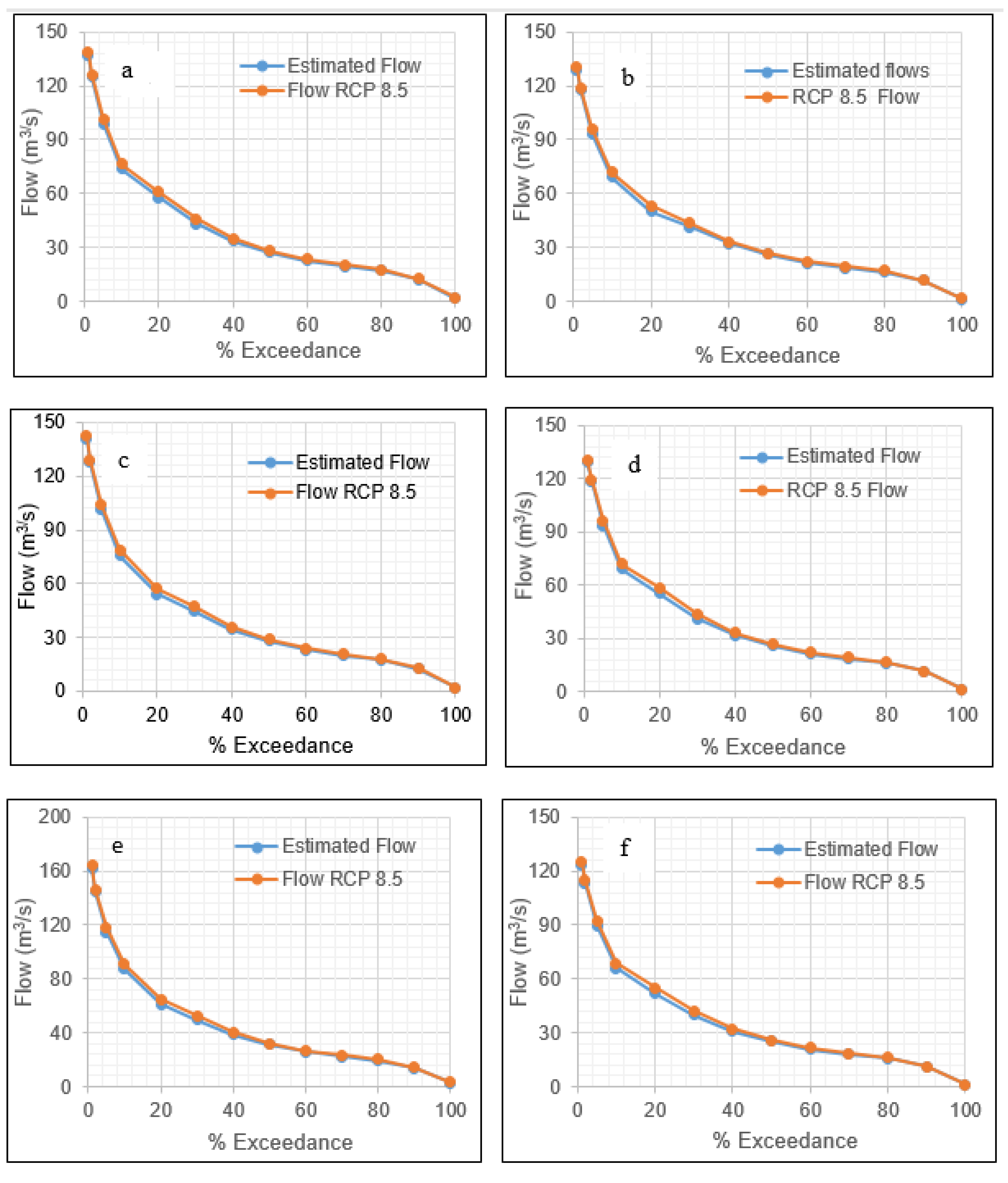
3.4. Derived Flow Duration Curves for Ungauged Sites

Six ungauged sites were selected in this study to explore their potential for hydropower generation for estimated observed flows and impact of climate change. Their selection was based on the geometric properties extracted from DEM and the community settlement pattern. Flow transfer from the gauged sites to the ungauged sites was achieved through the regional Flow Duration Curve. The drainage area ratio method was applied due to its wide use in the estimation of flows in ungauged catchments that had similar characteristics with the gauged catchments.
The physiographic properties of the sub-catchments were characterized by similar drainage areas and shapes, rainfall, relief expression, lithology and geology, land use/land cover, vegetation and aspect [46]. The gauged data from the index sites (gauged sites) were used to extrapolate the flows for the nearest ungauged sites. A simple linear regression method was used to derive the FDC for the ungauged sites, with drainage and flow being the major variables. Figure 10 illustrates the derived Flow Duration Curves for the ungauged sites.
Similar trends and shapes of the FDCs are repeated in the ungauged sites with less than 0.5 m3/s at Q100. The lower flows can also be attributed to the corresponding small catchments. The flows are higher from Q0–Q10, which is a direct response from a rainfall event, while medium flows begin from Q20–Q60 and low-to-drought flows range from Q60–Q100, which are also baseflows.

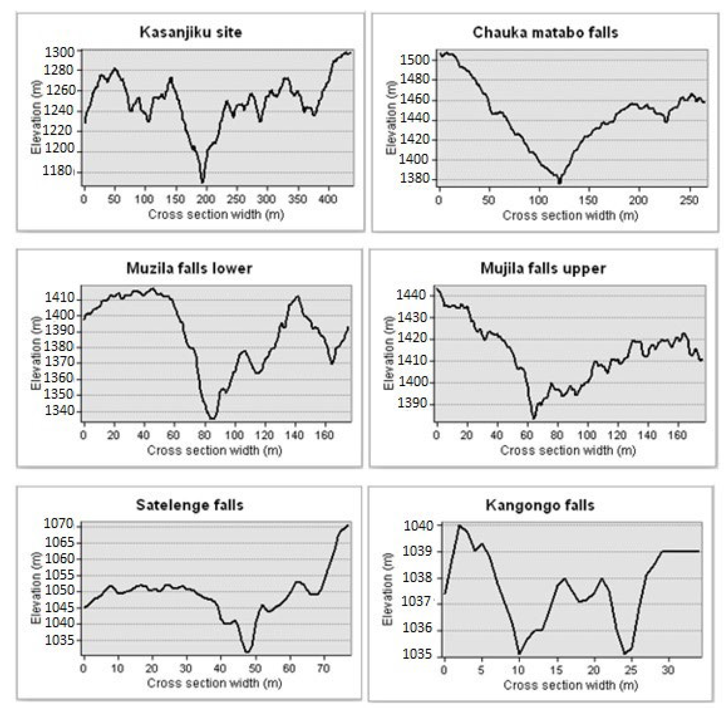
3.5. Elevation Profiles for Ungauged Sites in the Basin

The basin has 10 gauged sites, but only 6 sites had sufficient flow data used for deriving regional FDCs for application on ungauged sites. In this paper, the focus is made on six ungauged sites considered to have potential for hydropower generation.
The sites were further analyzed for elevation profiles in GIS to estimate the head of water to be used in the calculation of the hydropower potential. The higher the elevation at the site, the better the potential head of water downstream at the generation station. The head is expected to be increased with the construction of a weir at a narrow cross-section of the river. The distance of conveyance of water from the weir to the turbine house (generation house) is within 3–8 km. Therefore, the selection of hydropower potential sites must be carefully considered by taking into account the design criteria.
Many gauged sites have sufficient head but do not have a reasonable cross-section, width or length of flow conveyance to a possible generation station. Hence, most of the gauged sites could not meet the design criteria. They were, however, used for transferring observed and RCP 8.5 flows to ungauged site to facilitate the estimation of the hydropower potential. Six ungauged sites were selected based on the design criteria and were found to be suitable. The elevation profiles were then generated for each site from DEM in GIS and they show the height difference between the riverbed and the highest riverbanks. They also show the possible valley for water storage if a weir is constructed. Figure 11 illustrates the elevation profiles of the ungauged sites.

3.6. Hydropower Potential Sites

Based on the processed DEM, six sites were located in the basin. The site elevation (head) with reference to the possible hydropower station ranged from 4–40 m. This is the ground elevation difference (head) between the selected potential site and the possible hydropower station. Most of the potential sites were located on small falls or headwaters of the sub-catchments. The head may be achieved with the construction of weirs for an increased potential. The sites may be suitable for Run-Of-River (ROR) generation systems, as there is additional head between the sites and the possible locations for a generation station. The estimated hydropower potential under the impact of climate change for RCP 8.5 was based on the site elevation head and calculated using Equation (1), with a turbine efficiency of 80%. Table 4 shows the projected flows together with the hydropower projections for the baseline and future periods.
Table 4 shows that the hydropower potential for the ungauged sites is likely to increase between 5–10% on average under climate change for RCP 8.5 for the future period of 2021–2050. The change is because of the direct relationship of flow and hydropower potential. The flow for RCP 4.5 was not calculated as there were insignificant differences with the baseline and, hence, no differences on the hydropower potential.

4. Discussion

The study has shown that the impact of climate change on streamflow under RCP 4.5 may be slightly less than the baseflow. The trend and magnitude of simulated streamflow, as shown in the figures, is slightly less than the baseline period. The flow regime estimated for the ungauged catchments using the novel integrated approach shows that the hydropower potential is likely somewhat reduced for the future period. The results agree with the findings that the streamflow under RCP 4.5 may be less than the streamflow under the baseline [54,55]. The findings are also within predictions where different combinations of climate change and water use showed that the relative impacts are quite different across the whole Zambezi River basin [56,57]. Climate change projections contain large uncertainties, including external factors such as greenhouse gas emissions and changes in land use [58]. The uncertainty in the future simulation results remains hugely dependent upon the source of the climate change data and the change signals given by them. The results of the climate change impact on water resources have continued to be different across the Zambezi River basin in Southern Africa. However, the study has demonstrated that the streamflow will significantly remain the same and therefore hydropower potential will also be unaltered.
The simulated streamflow shows some minor variations from the baseline in the FDC under RCP 8.5. This may lead to a slight improvement in the hydropower potential for the selected sites, while other sites may experience a reduced potential depending on the season. The minor variations between the baseline and RCP 4.5 may be due to the smaller differences in RCPs at the beginning of the century (2020–2040) that entail less impact, while towards the end of the century (2040–2100), the RCP differences are wide and entail more impact. The FDCs constructed for the gauged sites were similar to the FDCs for the ungauged sites because the catchments have similar characteristics. The technique of an integrated approach involving the derivation of regional FDC, GIS and regression analysis was applied to obtain the FDC for the ungauged sites for the estimation of mini-hydropower potential. This was a novel approach in the Kabompo River Basin within the Zambezi River basin of Southern Africa. Similar results on a continental scale for hydropower generation potential were obtained after an evaluation of 712,615 km of river network spanning over 44 countries using an open-source geospatial database [7]. It is clear that many studies have concentrated on mega-hydropower generation potential, leaving out mini-hydropower estimations in the region. It is imperative to devise techniques such as the novel approach to help estimate mini-hydropower generation for the rural communities in the developing countries. The integrated approach demonstrated in this paper could be useful in the estimation of mini-hydropower potential in data scarce regions.

Limitations of the Study

A lack of data availability for validation in many sites was a challenge in estimating the hydropower potential. The estimation of hydropower potential was restricted to a few ungauged sites, which were near the gauged sites. The cost estimates of the power generation at the selected sites could not be done due to a lack of observed data.

5. Conclusions

The application of an integrated methodological approach on the use of regional FDCs, linear regression and GIS to estimate flows and potential head for the design of hydropower for the ungauged sites is a novelty in the Kabompo River Basin and has shown promising results in developing countries.
The FDC has confirmed that the peak flows are between Q0 and Q10, where there is a very steep slope with very high flows. The predicted flows at Q10 occur for about 10% of the time in a year. Therefore, the high flows (floods) are likely to last for one month and two weeks before subsiding. In addition, the basin has sufficient low flows at Q95, which is sustained by baseflows. The Q0–Q10 flows would be suitable for the design and estimation of the cost of a turbine for higher hydropower generation capacity, but only during the peak flow seasons in the ungauged sites
The FDC under the RCP 4.5 climate change scenario indicates insignificant change when compared with the baseline and therefore no change in hydropower potential. The FDC under the RCP 8.5 climate scenario confirmed that the peak flows are between Q0–Q10, where there is a very steep slope with very high flows. The predicted flows at Q10 occur for about 10% of the time in a year.
The FDC under RCP 8.5 confirmed that Q70–Q100 flows are reliable and sufficient for the design of small hydropower generation. The use of Q80 for design was preferred because of the fact that it would be available for 80% of the time in a year with very limited interruptions of generated power supply. It is envisaged that the estimated hydropower potential, if exploited at various sites in the rural part of the basin, would contribute to poverty reduction in many ways. The future research needs will be to focus on the impact of climate change on river flows for the period 2051–2100.

Author Contributions

Conceptualization, G.Z.N. and Y.E.W.; methodology, G.Z.N. and Y.E.W.; software, G.Z.N.; validation, G.Z.N. and Y.E.W.; formal analysis, G.Z.N. and Y.E.W.; investigation, G.Z.N. and Y.E.W.; data curation, G.Z.N.; writing—original draft preparation, G.Z.N.; writing review and editing, Y.E.W.; visualization, G.Z.N. All authors have read and agreed to the published version of the manuscript.

Funding

This research received no external funding.

Conflicts of Interest

The authors declare no conflict of interest.

References

  1. International Energy Agency (IEA). Assessment Methods for Small-Hydro Projects. Implementing Agreement for Hydropower. 2000. Available online: https://www.ieahydro.org/media/c617f800/Assessment%20Methods%20for%20Small-Hydro%20Projects.pdf (accessed on 25 January 2020).
  2. Galletti, A.; Avesani, D.; Bellin, A.; Majone, B. Detailed simulation of storage hydropower systems in large Alpine watersheds. J. Hydrol. 2021, 603, 127125. [Google Scholar] [CrossRef]
  3. Reichl, F.; Hack, J. Derivation of flow duration curves to estimate hydropower generation potential in data-scarce regions. Water 2017, 9, 572. [Google Scholar] [CrossRef]
  4. Sharma, N.K.; Tiwari, P.K.; Sood, Y.R. A comprehensive analysis of strategies, policies and development of hydropower in India: Special emphasis on small hydro power. Renew. Sustain. Energy Rev. 2013, 18, 460–470. [Google Scholar] [CrossRef]
  5. Macaringue, D. The Potential for Micro-Hydro Power Plants in Mozambique; University of KwaZulu-Natal: Pietermaritzburg, South Africa, 2009. [Google Scholar]
  6. Yüksel, I. Hydropower in Turkey for a clean and sustainable energy future. Renew. Sustain. Energy Rev. 2008, 12, 1622–1640. [Google Scholar] [CrossRef]
  7. Korkovelos, A.; Mentis, D.; Siyal, S.H.; Arderne, C.; Rogner, H.; Bazilian, M.; Howells, M.; Beck, H.; De Roo, A. A Geospatial Assessment of Small-Scale Hydropower Potential in Sub-Saharan Africa. Energies 2018, 11, 3100. [Google Scholar] [CrossRef]
  8. Yin, J.; Guo, S.; Gentine, P.; Sullivan, S.C.; Gu, L.; He, S.; Chen, J.; Liu, P. Does the hook structure constrain future flood intensification under anthropogenic climate warming? Water Resour. Res. 2021, 57, e2020WR028491. [Google Scholar] [CrossRef]
  9. Bevacqua, E.; Maraun, D.; Vousdoukas, M.I.; Voukouvalas, E.; Vrac, M.; Mentaschi, L.; Widmann, M. Higher probability of compound flooding from precipitation and storm surge in Europe under anthropogenic climate change. Sci. Adv. 2019, 5, eaaw5531. [Google Scholar] [CrossRef] [PubMed]
  10. Arias, M.E.; Farinosi, F.; Hughes, D.A. Future Hydropower Operations in the Zambezi River Basin: Climate Impacts and Adaptation Capacity. In River Research and Application; John Wiley & Sons: Hoboken, NJ, USA, 2022. [Google Scholar] [CrossRef]
  11. Hamududu, B.H.; Killingtveit, Å. Hydropower Production in Future Climate Scenarios; the Case for the Zambezi River. Energies 2016, 9, 502. [Google Scholar] [CrossRef]
  12. Stevanato, N.; Rocco, M.V.; Giuliani, M.; Castelletti, A.; Colombo, E. Advancing the representation of reservoir hydropower in energy systems modelling: The case of Zambesi River Basin. PLoS ONE 2021, 16, e0259876. [Google Scholar] [CrossRef] [PubMed]
  13. Yamba, F.D.; Walimwipi, H.; Jain, S.; Zhou, P.; Cuamba, B.; Mzezewa, C. Climate change/variability implications on hydroelectricity generation in the Zambezi River Basin. Mitig. Adapt. Strateg. Glob. Chang. 2011, 16, 617–628. [Google Scholar] [CrossRef]
  14. Searcy, J.K. Flow-Duration Curves Flow-Duration Curves. Manual of Hydrology Part 2. Low-Flow Techniques. Geological Survey Water-Supply Paper. 1969. Available online: https://pubs.usgs.gov/wsp/1542a/report.pdf (accessed on 30 April 2020).
  15. Karamouz, M.; Szidarovszky, F.; Zahraie, B. Water Resources Systems Analysis with Emphasis on Conflict Resolution; Lewis Publishers: New York, NY, USA; Washington, DC, USA, 2003; 608p. [Google Scholar]
  16. Mousavi, R.S.; Ahmadizadeh, M.; Marofi, S. A Multi-GCM assessment of the climate change impact on the hydrology and hydropower potential of a semi-arid basin (A Case Study of the Dez Dam Basin, Iran). Water 2018, 10, 1458. [Google Scholar] [CrossRef]
  17. Botai, C.M.; Botai, J.O.; Muchuru, S.; Ngwana, I. Hydrometeorological Research in South Africa: A Review. Water 2015, 7, 1580–1594. [Google Scholar] [CrossRef]
  18. Euroconsult, M.M. Integrated Water Resources Management Strategy and Implementation Plan for the Zambezi River Basin. 2008. Available online: http://zambezicommission.org/sites/default/files/clusters_pdfs/Zambezi%20River_Basin_IWRM_Strategy_ZAMSTRAT.pdf (accessed on 20 January 2021).
  19. Hughes, D.A. Comparison of satellite rainfall data with observations from gauging station networks. J. Hydrol. 2006, 327, 399–410. [Google Scholar] [CrossRef]
  20. Gómez-Llanos, E.; Arias-Trujillo, J.; Durán-Barroso, P.; Ceballos-Martínez, J.M.; Torrecilla-Pinero, J.A.; Urueña-Fernández, C.; Candel-Pérez, M. Department, Hydropower Potential Assessment in Water Supply Systems. Proceedings 2018, 2, 1299. [Google Scholar] [CrossRef]
  21. International Finance Corporation (IFC). Hydroelectric Power, A Guide for Developers and Investors; World Bank: Washington, DC, USA, 2012; pp. 145–152. [Google Scholar] [CrossRef]
  22. Samora, I.; Manso, P.; Franca, M.J.; Schleiss, A.J.; Ramos, H.M. Energy Recovery Using Micro-Hydropower Technology in Water Supply Systems: The Case Study of the City of Fribourg. Water 2016, 8, 344. [Google Scholar] [CrossRef]
  23. Van Dijk, M.; van Vuuren, S.J.; Bhagwan, J.N. Conduit Hydropower Potential In A City’s Water Distribution System, Imesa papers. 2012, Volume 12, pp. 1–16. Available online: https://imesa.org.za/wp-content/uploads/2015/08/Conduit-hydropower-potential-in-a-citys-water-distribution-system-Prof-Marco-van-Dyk-University-of-Pta.pdf (accessed on 14 April 2022).
  24. Jung, S.; Bae, Y.; Kim, J.; Joo, H.; Kim, H.; Jung, J. Analysis of Small Hydropower Generation Potential: (1) Estimation of the Potential in Ungaged Basins. Energies 2021, 14, 2977. [Google Scholar] [CrossRef]
  25. Ndhlovu, G.; Woyessa, Y. Use of gridded climate data for hydrological modelling in the Zambezi River Basin, Southern Africa. J. Hydrol. 2021, 602, 126749. [Google Scholar] [CrossRef]
  26. World Bank. The Zambezi River Basin–A multi-sector investment opportunity analysis. Modeling Anal. Input Data 2010, 4, 158. [Google Scholar]
  27. Kapangaziwiri, E.; Mokoena, M.P.; Kahinda, J.M.; Hughes, D.A. ECOMAG: An Evaluation for Use in South Africa. 2013. Available online: http://www.wrc.org.za/wp-content/uploads/mdocs/TT%20555-13.pdf (accessed on 12 February 2021).
  28. Young, T.; Tucker, T.; Galloway, M.; Manyike, P. Climate Change and Health in SADC. September 2010. Available online: https://open.umich.edu/sites/default/files/downloads/uct-ccandhealth220910.pdf (accessed on 5 October 2020).
  29. Senent-Aparicio, J.; Jimeno-Sáez, P.; López-Ballesteros, A.; Giménez, J.G.; Pérez-Sánchez, J.; Cecilia, J.M.; Srinivasan, R. Impacts of swat weather generator statistics from high-resolution datasets on monthly streamflow simulation over Peninsular Spain. J. Hydrol. Reg. Stud. 2021, 35, 2021. [Google Scholar] [CrossRef]
  30. Taylor, K.E.; Stouffer, R.J.; Meehl, G.A. An Overview of CMIP5 and the Experiment Design. Bull. Am. Meteorol. Soc. 2012, 93, 485–498. [Google Scholar] [CrossRef]
  31. Gassman, P.P.W.; Reyes, M.M.R.; Green, C.C.H.; Arnold, J.J.G. The Soil and Water Assessment Tool: Historical development, applications, and future research directions. Trans. ASAE 2007, 50, 1211–1250. [Google Scholar] [CrossRef]
  32. Moriasi, D.N.; Arnold, J.G.; van Liew, M.W.; Bingner, R.L.; Harmel, R.D.; Veith, T.L. Model Evaluation Guidelines For Systematic Quantification of Accuracy in Watershed Simulations. Am. Soc. Agric. Biol. Eng. 2007, 50, 885–900. [Google Scholar]
  33. Odusanya, A.E.; Mehdi, B.; Schürz, C.; Oke, A.O.; Awokola, O.S.; Awomeso, J.A.; Adejuwon, J.O.; Schulz, K. Multi-site calibration and validation of SWAT with satellite-based evapotranspiration in a data-sparse catchment in southwestern Nigeria. Hydrol. Earth Syst. Sci. 2019, 23, 1113–1144. [Google Scholar] [CrossRef]
  34. Trzaska, S.; Schnarr, E. A Review of Downscaling Methods for Climate Change Projections. African and Latin American Resilience to Climate Change (ARCC); United States Agency for International Development by Tetra Tech ARD: Arlington, VA, USA, 2014; pp. 1–42. [Google Scholar] [CrossRef]
  35. Anandhi, A.; Frei, A.; Pierson, D.C.; Schneiderman, E.M.; Zion, M.S.; Lounsbury, D.; Matonse, A.H. Examination of change factor methodologies for climate change impact assessment. Water Resour. Res. 2011, 47, W03501. [Google Scholar] [CrossRef]
  36. Vogel, R.M.; Fennessey, N.M. Flow Duration Curves II: A Review of Applications in Water Resources Planning1. JAWRA J. Am. Water Resour. Assoc. 1996, 31, 1029–1039. [Google Scholar] [CrossRef]
  37. Yildiz, V.; Vrugt, J.A. A toolbox for the optimal design of run-of-river hydropower plants. Environ. Model. Softw. 2018, 111, 134–152. [Google Scholar] [CrossRef]
  38. Wali, U.G. Estimating hydropower potential of an ungaged stream. Int. J. Emerg. Technol. Adv. Eng. 2013, 3, 592–600. Available online: www.ijetae.com (accessed on 20 June 2022).
  39. Mülle, M.F.; Thompson, S.E. Stochastic or statistic? Comparing flow duration curve models in ungauged basins and changing climates. Hydrol. Earth Syst. Sci. Discuss. 2015, 12, 9765–9811. [Google Scholar] [CrossRef]
  40. Ngongondo, C.; Li, L.; Gong, L.; Xu, C.-Y.; Alemaw, B.F. Flood frequency under changing climate in the upper Kafue River basin, Southern Africa: A large scale hydrological model application. Stoch. Environ. Res. Risk Assess. 2013, 27, 1883–1898. [Google Scholar] [CrossRef]
  41. Verma, R.K.; Murthy, S.; Verma, S.; Mishra, S.K. Design flow duration curves for environmental flows estimation in Damodar River Basin, India. Appl. Water Sci. 2017, 7, 1283–1293. [Google Scholar] [CrossRef]
  42. Smakhtin, V.U. Low Flow Hydrology: A review. J. Hydrol. 2001, 240, 147–186. Available online: http://researchspace.csir.co.za/dspace/bitstream/id/1386/smakhtin_2001.pdf/;jsessionid=9F469DEA00D334B3E35271529B391A38 (accessed on 19 April 2022). [CrossRef]
  43. Smakhtin, V.Y. Simple Methods Hydrological Data Provision, Integrated and Application of Daily Flow Analysis and Simulation Approaches Within Southern Africa; Water Research Commission (WRC); WRC Report No. 867/1/00. 2000. Available online: http://www.wrc.org.za/wp-content/uploads/mdocs/867-1-00.pdf (accessed on 14 April 2022).
  44. Leroy, F.; Heitz, P.E.; Khosrowpanah, P.E.S. Prediction of Flow Duration Curves for Use in Hydropower Analysis at Ungaged Sites in Kosrae, FSM; Technical Report No. 137; University of Guam Water and Environmental Research Institute of the Western Pacific UOG Station: Mangilao, GU, USA, 2012. [Google Scholar]
  45. Nruthya, K.; Srinivas, V.V. Evaluating Methods to Predict Streamflow at Ungauged Sites Using Regional Flow Duration Curves: A Case Study. Aquat. Procedia 2015, 4, 641–648. [Google Scholar] [CrossRef]
  46. USDA. Estimating Design Stream Flows at Road-Stream Crossings. In Stream Simulation: An Ecological Approach to Providing Passage for Aquatic Organisms at Road-Stream Crossings; U.S. Department of Agriculture: Washington, DC, USA, 2008. [Google Scholar]
  47. Mohamoud, Y.M. Prediction of daily flow duration curves and streamflow for ungauged catchments using regional flow duration curves. Hydrol. Sci. J. 2008, 53, 706–724. [Google Scholar] [CrossRef]
  48. Joel, N.; Ndayizeye, J.; Mkhandi, S. Regional Flow Duration Curve Estimation and its Application in Assessing Low Flow Characteristics for Ungauged Catchment. A Case Study of Rwegura Catchment-Burundi. Nile Basin Water Sci. Eng. J. 2011, 4, 14–23. Available online: https://nbcbn.net/ctrl/images/img/uploads/1209_06113847.pdf (accessed on 14 April 2022).
  49. Abbaspour, K.C.; Rouholahnejad, E.; Vaghefi, S.; Srinivasan, R.; Yang, H.; Kløve, B. A continental-scale hydrology and water quality model for Europe: Calibration and uncertainty of a high-resolution large-scale SWAT model. J. Hydrol. 2015, 524, 733–752. [Google Scholar] [CrossRef]
  50. Nash, J.E.; Sutcliffe, J.V. River Flow Forecasting Through Conceptual Models Part I-a Discussion of Principles. J. Hydrol. 1970, 10, 282–290. [Google Scholar] [CrossRef]
  51. Gunathilake, M.B.; Amaratunga, Y.V.; Perera, A.; Chathuranika, I.M.; Gunathilake, A.S.; Rathnayake, U. Evaluation of Future Climate and Potential Impact on Streamflow in the Upper Nan River Basin of Northern Thailand Miyuru. Adv. Meteorol. 2020, 2020, 8881118. [Google Scholar] [CrossRef]
  52. Mello, C.; Vieira, N.; Guzman, J.; Viola, M.; Beskow, S.; Alvarenga, L. Climate Change Impacts on Water Resources of the Largest Hydropower Plant Reservoir in Southeast Brazil. Water 2021, 13, 1560. [Google Scholar] [CrossRef]
  53. Novara, D.; McNabola, A. Design and Year-Long Performance Evaluation of a Pump as Turbine (PAT) Pico-Hydropower Energy Recovery Device in a Water Network. Water 2021, 13, 3014. [Google Scholar] [CrossRef]
  54. Hamududu, B.H. Impacts of Climate Change on Water Resources and Hydropower Systems in Central and Southern Africa; Norwegian University of Science and Technology: Trondheim, Norway, 2012. [Google Scholar]
  55. Ndhlovu, G.Z.; Woyessa, Y.E. Evaluation of Streamflow under Climate Change in the Zambezi River Basin of Southern Africa. Water 2021, 13, 3114. [Google Scholar] [CrossRef]
  56. Hughes, D.A.; Farinosi, F. Assessing development and climate variability impacts on water resources in the Zambezi River basin. Simulating future scenarios of climate and development. J. Hydrol. Reg. Stud. 2020, 32, 100763. [Google Scholar] [CrossRef] [PubMed]
  57. Fant, C.; Gebretsadik, Y.; McCluskey, A.; Strzepek, K. An uncertainty approach to assessment of climate change impacts on the Zambezi River Basin. Clim. Chang. 2015, 130, 35–48. [Google Scholar] [CrossRef]
  58. Sainz, S.G. The Zambezi River Basin: Water Resources Management Energy-Food-Water Nexus Approach. Master’s Thesis, Department of Physical Geography, Stockholm University, Stockholm, Sweden, 2018. [Google Scholar]
Figure 1. (a) Location of Kabompo River Basin in Southern Africa. (b) Distribution of gauged and ungauged sites.
Hydrology 09 00149 g001
Figure 2. Flow chart of the methodological approach.
Hydrology 09 00149 g002
Figure 3. Calibration of SWAT model.
Hydrology 09 00149 g003
Figure 4. Validation of SWAT model.
Hydrology 09 00149 g004
Figure 5. Flow Duration Curves for ensemble streamflow under baseline period.
Hydrology 09 00149 g005
Figure 6. Flow Duration Curves for ensemble streamflow under RCP 4.5.
Hydrology 09 00149 g006
Figure 7. Flow Duration Curves for ensemble streamflow under RCP 8.5.
Hydrology 09 00149 g007
Figure 8. Flow Duration Curves of ensemble means for RCP 8.5, RCP 4.5 and observed flow.
Hydrology 09 00149 g008
Figure 9. (a) Watopa gauge site with observed flow from 1978–2005, (b) Kabompo boma gauge site with observed flow from 1950–1993, (c) Luakela gauge site with observed flow from 1970–2014, (d) Mumbezhi gauge site with observed flow from 1971–2013, (e) West Lunga gauge site with observed flow from 1954–1970 and (f) Manyinga gauge site with observed flow from 1961–1992.
Hydrology 09 00149 g009
Figure 10. (a) Mujila falls lower site with estimated flows, (b) Mujila falls upper site with estimated flows, (c) Kasanjiku falls site with estimated flows, (d) Chauka Matambu falls with estimated flows, (e) Satelenge falls with estimated flows and (f) Kangongo falls with estimated flows.
Hydrology 09 00149 g010
Figure 11. Elevation profiles of the cross-sections at ungauged sites.
Hydrology 09 00149 g011
Table 1. The GCMs used in this study.
CountryResearch CenterGCMResolution
Lat Long Degrees
FranceCentre National de Recherches MétéorologiquesCNRM-CM51.4 × 1.4
FranceInstitute Pierre Simon LaplaceIPCL-CM5A-LR3.7 × 1.9
JapanCenter for Climate Research System (The University of Tokyo), National Institute for Environmental Studies and Frontier Research Center for Global Change (JAMSTEC)MIROC51.4 × 1.4
GermanyMax Planck Institute for MeteorologyMPI-ESM-MR1.9 × 1.9
JapanMeteorological Research InstituteMRI-CGCM31.4 × 1.4
Table 2. Calibration parameters.
Parameter NameDescriptiont-Statp-Value
R__SOL_AWC (.).solAvailable water capacity of the soil layer (mm H2O/mm soil)−7.6150.000
R__HRU_SLP.hruAverage slope steepness (fraction)−2.1710.030
R__SOL_BD (.).solSoil bulk density−2.1260.033
R__SOL_K (.).solSaturated hydraulic conductivity (mm/hour)−2.0320.042
V__GW_DELAY.gwGroundwater delay (days)−1.8120.071
V__CH_K2.rteManning’s n value for the main channel−1.2390.215
R__SLSUBBSN.hruAverage slope length (m)1.0570.291
R__OV_N.hruManning’s n value for overland flow−1.0310.303
V__ALPHA_BNK.rteBase flow alpha factor for bank storage (days)−0.8220.411
V__ALPHA_BF.gwBase flow alpha factor (days)−0.7770.437
V__GWQMN.gwThreshold depth of water in the shallow aquifer required for return flow to occur (mm)0.56360.573
R__CN2.mgtSCS runoff curve number0.5250.599
V__CH_N2.rteManning’s n value for the main channel−0.3820.703
V__SURLAG.bsnSurface runoff lag time (days)−0.3400.734
V__REVAPMN.gwThreshold depth of water in the shallow aquifer for “revap” to occur (mm)−0.3140.753
R__SOL_ZMX.solMax depth from soil surface to rooting depth (mm)−0.1820.856
V__ESCO.hruPlant uptake compensation factor0.1220.903
V__GW_REVAP.gwGroundwater “revap” coefficient0.0360.971
Table 3. Calibration and validation of SWAT model.
ParameterData PeriodR2NSP-FactorR-Factor
Calibration1982–19970.730.730.750.75
Validation1998–20050.700.640.730.55
Table 4. The projected flows with their hydropower projections for the future.
Hydropower Potential Site
(Ungauged)
Area (km2)Potential
Height(m)
Estimated
Design
Flow (m3/s)
RCP 8.5
Design Flow (m3/s)
Estimated Potential
Gen Capacity (KW)
Future Potential
Gen Capacity RCP 8.5 (KW)
Mujila falls lower site501.044016.3216.9751235327
Mujila falls upper site1275.983017.0917.7740244184
Kasanjiku falls site1625.114017.4418.1454755695
Chauka Matambu fall site555.034016.3717.0251395343
Satelenge Falls3598.221519.4120.1922852377
Kangongo Falls0.3415.8116.45496516
Publisher’s Note: MDPI stays neutral with regard to jurisdictional claims in published maps and institutional affiliations.

