

Daily Streamflow Forecasting in Mountainous Catchment Using XGBoost, LightGBM and CatBoost

Institute of Geological Sciences, Faculty of Geography and Geology, Jagiellonian University, 30-387 Cracow, Poland
Hydrology 2022, 9(12), 226; https://doi.org/10.3390/hydrology9120226
Submission received: 7 November 2022
/
Revised: 6 December 2022
/
Accepted: 7 December 2022
/
Published: 13 December 2022
(This article belongs to the Special Issue Stochastic and Deterministic Modelling of Hydrologic Variables)
Abstract
:Streamflow forecasting in mountainous catchments is and will continue to be one of the important hydrological tasks. In recent years machine learning models are increasingly used for such forecasts. A direct comparison of the use of the three gradient boosting models (XGBoost, LightGBM and CatBoost) to forecast daily streamflow in mountainous catchment is our main contribution. As predictors we use daily precipitation, runoff at upstream gauge station and two-day preceding observations. All three algorithms are simple to implement in Python, fast and robust. Compared to deep machine learning models (like LSTM), they allow for easy interpretation of the significance of predictors. All tested models achieved Nash-Sutcliffe model efficiency (NSE) in the range of 0.85–0.89 and RMSE in the range of 6.8–7.8 ms. A minimum of 12 years of training data series is required for such a result. The XGBoost did not turn out to be the best model for the daily streamflow forecast, although it is the most popular model. Using default model parameters, the best results were obtained with CatBoost. By optimizing the hyperparameters, the best forecast results were obtained by LightGBM. The differences between the model results are much smaller than the differences within the models themselves when suboptimal hyperparameters are used.
1. Introduction
1.1. Streamflow Forecasting
Streamflow forecasting is crucial component of effective flood protection and water management. A reliable streamflow forecast is still one of the main goals of hydrological research [1]. Scientists and practitioners are interested in both extreme events, such as floods and droughts, and medium flows. In practice, however, forecasting models seem to be used and verified in relation to one specific type of task, such as prediction of low flows [2] or drought forecasting [3]. Forecasting a wide spectrum of streamflows with one model is not an easy task and few models have such a wide range of applicability [4].
Mountainous rivers, due to the high flow dynamics, are particularly prone to the risk of flooding, but flood modeling in such areas is extremely difficult [5]. The source of these difficulties is complex topography, shorter concentration times of flood waves and the local nature of extreme rainfall, often limited to only one or several mountain valleys [6]. Traditional physical models describe the individual processes that transform rainfall into runoff. The streamflow prediction horizon depends on the purpose of the forecast. Violent phenomena, such as floods, are usually forecasted in a shorter horizon—hours or days. Long-term forecast of streamflow (days-months) is usually made for the needs of water management, to balance water resources [7]. The presented analysis is based on daily runoff and precipitation data. The runoff forecast is also generated on a daily basis. This is adapted to mountainous catchments where the times to peak in flood waves are shorter than in lowlands.
The rapid development of data-driven hydrological models in recent years allows us to look at streamflow forecasting problem from a different perspective, also in the area of water management [8]. Physically-based hydrological models capture simplified representations of the physical processes that underlie streamflow, while data driven approaches can provide more accurate predictions [9], mainly due to better possibilities of modeling non-linear dependencies [10]. Although traditional forecasting methods based on the description of physical processes have many advantages, the scientists are beginning to see the potential of data-driven models, including Machine Learning (ML) algorithms [11]. Data-driven models may try to replace classical models, but there are also attempts to use them in conjunction with classical models [12].
1.2. Data-Driven Models
In traditional hydrological models, the role of data is of secondary importance. The focus is on conceptual or physical representation of the phenomena that use data mainly for models calibration purposes. In the case of data-driven models, it is the data that determines the model itself. Machine learning, which has become popular in recent years, uses the concept of data-driven models and find practical application in many areas of science, including hydrology [1,13]. Machine learning models are successfully used for forecasting evapotranspiration [1], precipitation [14], soil moisture [15], groundwater levels and streamflow [1,16,17,18]. As found by [16] ensemble model strategies are superior over the regular (individual) model learning in hydrology. Currently, there are many data-driven models available, ranging from simple models to models that require significant computing power. The simplest models are, for example, regression models, while the most advanced models include deep machine learning models. The best results of streamflow forecasting are currently obtained from recursive and deep models, such as LSTM [17,18]. However, this type of deep learning models is typically criticized for a lack of interpretability [19]. In the pursuit of better models, one of the essential goals of prediction can be lost—model interpretability. Model interpretability is the ability to correctly interpret a prediction model’s output [20]. It engenders appropriate user trust, provides insight into how a model may be improved, and supports understanding of the process being modeled. The SHAP (SHapley Additive exPlanations) model [20] assigns each feature an importance value for a particular prediction.
The selection of appropriate meteorological, hydrological and geomorphological parameters (called features) for the data-model is extremely important. It is found that ML models could fail in predicting streamflow from only meteorological variables in the absence of past values of streamflow due to the lagged relationships between streamflow and meteorological variables [18]. This is directly related to the interpretability of the model, as only for models with such a feature can the set of input parameters be appropriately selected.
In this paper, we present an analysis of state-of-the-art data-driven models that are interpretable. Thus, the models of deep machine learning were omitted, the results of interpretability of which are still in the realm of research by many authors. The simplest models, such as Multiple Linear Regression (MLR), are often used as reference models [18]. The MLR and Random Forest (RF) were used as the base models to evaluate streamflow forecast results. Both are successfully used to model the water cycle elements—precipitation [21], evaporation [22] and rainfall-runoff modeling [23,24]. Random forests is simple and fast algorithm with high predictive performance, widely used in hydrological applications. A detailed research on the use of RF in hydrology has been prepared by [8].
Three popular models were selected for this research: XGBoost, LightGBM and CatBoost. Although the main area of application of the presented models are classification problems, they are also successfully used for regression tasks, including modeling various processes related to the water cycle. [25] used XGBoost for predicting ice phenomena in eight water gauges on the Warta River, Poland. [26] used XGBoost for stream temperature prediction in the Pacific Northwest and Mid-Atlantic regions.
Most of the authors found that more advanced models such as Convolutional Neural Networks (CNN) or Recurrent Neural Networks (RNN), give slightly better flow prediction results [13,18,27]. One of the most widely used RNN models is the Long Short-Term Memory (LSTM) [1]. Compared to other types of RNNs, LSTMs do not have a problem with exploding/vanishing gradients and can learn long-term dependencies between input and output features. However, there are studies showing that the XGBoost and LSTM models give similar forecast results [28]. This may mean that result depends on the features adopted for the construction of the ML model, and perhaps also on a specific implementation. A comprehensive review of deep learning applications in hydrology and water resources was prepared by [1]. An extensive and detailed comparison of the ensemble machine learning algorithms has been published by [16].
The Interpretable Artificial Intelligence (IAI) models are capable of unveiling the rationale behind the predictions while eXplainable Artificial Intelligence (XAI) models are capable of discovering new knowledge and justifying results, which are critical for enhanced accountability of data driven predictions [13]. The tree-based models presented in this paper are IAI model and can transform into XAI models when they are coupled with the explanatory methods such as the SHAP [20]. Machine learning models such as Convolutional Neural Networks (CNN) or Long Short-Term Memory (LSTM), which give slightly better flow prediction results, however, are not interpretable [13].
1.3. Aim of the Present Study
The aim of the study was to verify popular machine learning methods that are relatively easy to parameterize, interpretable and give results not much worse than state-of-the-art models. As found by [16], the boosting techniques (e.g., XGBoost, LGBoost) have been more frequent and successfully implemented in hydrological problems than the bagging (RF) approaches. The authors were not able to find in the literature a direct comparison of boosting algorithms to forecast daily streamflows. The most comprehensive comparison of decision tree-based models presented by [13] shows that scientists mainly develop improved versions of individual algorithms by comparing them with baseline versions, not with each other. The most frequently used model is XGBoost [16,29], but it is also the oldest model from the presented originating in year 2016. We decided to check whether the newer algorithms, LGBoost [30] from 2017 and CatBoost [31] from 2018, will provide better forecasts. While the XGBoost algorithm is still the most popular, CatBoost authors claims that their solution is not only much faster, but also gives better predictions [32]. The thesis of CatBoost’s better performance has been confirmed for big data work cases [33].
In the case of comparative analyzes, it is important to be able to verify the results for possibly undisturbed observations that can be easily repeated in other catchments. For this reason, a mountainous river catchment was selected for the analysis, with a possibly natural flow regime, not disturbed by, for example, retention reservoirs. As data source we decided to use only global projects with public data. Daily precipitation was derived from the ERA5 project [34], and the average daily streamflow observations from The Global Runoff Data Centre (Koblenz, Germany). Among the most commonly used streamflow predictors, such as precipitation, temperature, past (lagged) streamflows, evapotranspiration and vegetation indices, it was decided to use only two key parameters: precipitation and lagged streamflows. If non-informative predictor variables are included in the model, the performance of some algorithms (e.g., linear regression) may decrease considerably, while if too many predictor variables are included, the computational burden may become prohibitive [29]. Flow forecasts are calculated for gauged cross-sections, but as [35] proved, presented models can also be successfully used for ungauged catchments.
The subsequent sections of the manuscript are organized as follows. In Section 2 we present study area, data used and machine learning boosting methods implemented to predict runoff. Two baseline models named Multiple Linear Regression and Random Forest are used here as the reference. The Section 3 presents a comparison of daily streamflow forecasts for five analyzed models and three input data scenarios. An in-depth analysis of the results in the context of selected machine learning models is presented in the Section 4. The last Section 5 summarizes all the works.
2. Materials and Methods
2.1. Study Area
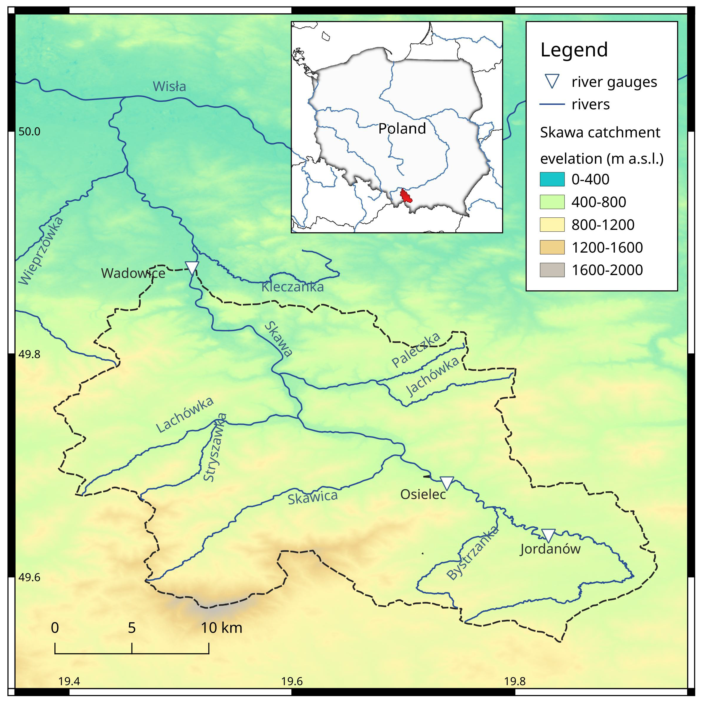
A mountainous Skawa River catchment with little land development, located in the Polish Carpathians, was selected as the research area. This region of Europe is at risk of both flooding [6] and drought [36,37]. The Skawa River is one of the most flood-prone mountain rivers in Polish Carpathians. Mean annual precipitation at Wadowice meteorological station in the period 1955–2014 was 816 mm [38]. Station in Wadowice recorded one of the highest number of anomalously high precipitation months in the region [39]. The highest monthly precipitation at Jordanów meteorological station exceeded 300 mm [40]. The mean snow cover duration for the period 1950–2018 is about 70 days, but with a tendency to systematically shorten due to climate change [41].
The Skawa River to Wadowice gauge station has catchment area of 835 km (Figure 1). The mean annual runoff at Wadowice gauge station from years 1961–1997 equals 12.7 ms, with mean annual flood runoff 242 ms [42]. This high ratio confirms mountainous characteristic of Skawa catchment from hydrological perspective. According research of [42], in the last century the minimum annual water stage of Skawa River at Wadowice station has lowered by more than 2 m. It is related to the erosion of the river bed and should not be understood as a decrease in flows.
From three gauge stations available in upper part of Skawa River we used two for this analysis—Osielec and Wadowice. Osielec cross-section located 34 km upstream from Wadowice (Figure 1) is treated as main source of upstream runoff data. The third gauge station (Jordanów) is omitted in this study because it is too close to the Osielec station (about 9 km).
The mean annual runoff calculated from longer observations used in this research equals 3.7 ms for gauge station Osielec (years 1970–2020) and 12.3 ms for Wadowice (years 1950–2020).
2.2. Data
All data used in the study come from public databases with a global reach. The source of the daily streamflow data is The Global Runoff Data Centre (GRDC), 56068 Koblenz, Germany. The GRDC operates under the auspices of the World Meteorological Organisation (WMO) and is lead by The German Federal Institute of Hydrology. The Global Runoff Database is a unique collection of river discharge data on a global scale. It contains time series of daily and monthly river discharge data of currently more than 9800 stations worldwide. The database is continuously updated by national hydrological services. The daily precipitation data comes from a reanalysis project ERA5 [34]. The data in this database covers the period from 1950 to 2–3 months before the present and are generated with a spatial resolution of approximately 9 km.
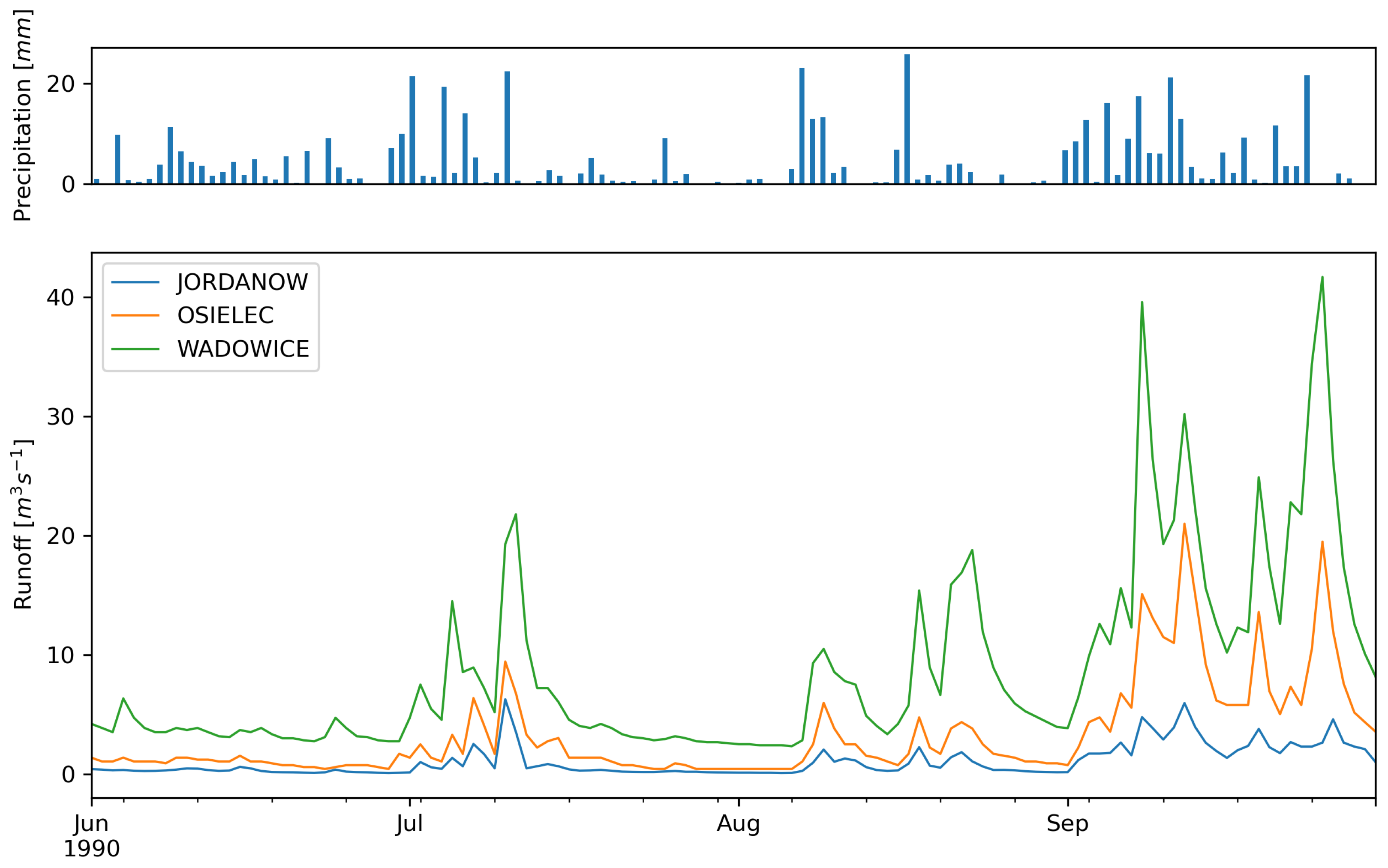
For model training we used 29 years of daily data from 1981–2009. A fragment of the data from 1990 is shown in the form of a hyetograph and hydrograph for three stations in Figure 2. For model evaluation we used 7 years of daily data from years 2010–2017. The scope of the data was limited to 2017, as the Świnna Poręba dam, located upstream Wadowice gauge station, was started to be filled in 2018, which had an impact on the course of hydrographs.
The daily streamflow in the Wadowice cross-section was the forecast value based on three scenarios, presented in Table 1. In Scenario 1, only current and historical precipitation data in the catchment area were used. In Scenario 2, only the current and historical data for the streamflow in the Osielec cross-section, located upstream from Wadowice, were used (Figure 1). The last scenario assumed the use of the previously mentioned data and, additionally, historical data from the Wadowice cross-section. Historical data should be understood as daily data from the previous day (named as lag1) and two days before (lag2) (Table 1).
2.3. Baseline Models
One linear regression model (Multiple Linear Regression) and one bagging-based model (Random Forest) were selected as benchmark algorithms.
2.3.1. Multiple Linear Regression (MLR)
The MLR approach predicts values of a dependent variable y when independent variables are given [43]. The MLR equation takes the following form:
where y is the dependent variable, a is the constant value or intercept of the regression line and y axis, is the amount the response variable y changes by the independent variables .
2.3.2. Random Forest (RF)
Random Forest is an ensemble of unpruned classification or regression trees created by using bootstrap samples of the training data and random feature selection in tree induction [44]. Prediction is made by aggregating (majority vote or averaging) the predictions of the ensemble. In the bagging algorithms, the decision trees run in parallel independently and do not interact with each other [13]. The bagging algorithms (including RT) are most suitable for problems with small training datasets [16].
2.4. Boosting Models
Gradient boosting models are an ensemble of weak classifiers or regressors (e.g., a decision tree model) where multiple weaker models are combined to produce a stronger model [13]. In the boosting algorithm, multiple trees are grown sequentially using the information from the existing trees. A new decision tree is generated by improving the performance of the tree generated in the previous iteration. All presented boosting models are implementations of Gradient Boosted Decision Tree (GBDT).
2.4.1. Extreme Gradient Boosting (XGBoost)
Extreme Gradient Boosting (also known as XGBoost) is a method based on gradient boosting proposed by [45]. In this technique, the decision trees classifier is commonly used as a weak model [16]. The predictions are created from weak learners that continuously improve the former learners. The XGBoost introduces the regularization term in the objective function to prevent overfitting
where O is objective function, denotes the regularization term at the k iteration time, and C is a constant. The regularization term is expressed as
where denotes complexity of leaves, H represents the number of leaves, denotes the penalty parameter, and is the output of each leaf node. The XGBoost splits the trees depth-wise or level-wise. Each tree (decision) computes the feature and corresponding threshold along with the best branch effect. Consecutive splits are performed to grow the tree structures.
2.4.2. Light Gradient Boosting Machine (LGBoost)
Light Gradient Boosting Machine (LightGBM or LGBoost) was proposed by [30]. This histogram-based algorithm increases the training speed and reduces memory consumption by trees leaf-wise growth strategy with a maximum depth limit. According to the level-wise growth strategy, the leaves on the same layer are simultaneously split. Leaves on same layer are indiscriminately treated, whereas they have different information gain. Information gain indicates the expected reduction in entropy caused by splitting the nodes based on attributes [46]
where is the information entropy of the collection B, is the ration of B pertaining to category d, D is the number of categories, is the value of attribute V, and is the subset of B for which attribute has value .
2.4.3. Categorical Boosting (CatBoost)
Categorical Boosting (also known as CatBoost) is a permutation-driven alternative to the classic algorithm, and an innovative algorithm for processing categorical features [31,32]. There are two new concepts in the proposed method: ordered target statistics and ordered boosting. An in-depth analysis of this algorithm in terms of classification and regression for different tasks was published by [33].
The use of CatBoost for regression problems in earth sciences (mainly meteorology) has been published [33], but we could not find a single example of a use for streamflow prediction.
2.5. Models Implementation
All selected ML models are implemented in the Python 3.10.4 language. The Scikit-learn 1.1.2 library [49] was used as the base library. Two models from this library were used as benchmark—LinearRegression and RandomForestRegressor. The following regressors were compared as part of the analysis: XGBRegressor 1.6.2 [45], LGBMRegressor 3.3.3 [30] and CatBoostRegressor 1.1 [31].
The modules of the Scikit-learn library were used for data preprocessing: transformation using the MinMaxScaler normalization function and the TimeSeriesSplit function for data split specific for time series. For model training we used 29 years of daily data from 1981–2009, which means 10,585 observations. For model evaluation we used 7 years of daily data from years 2010–2017, that is 2920 observations.
The baseline model comparison assumed the use of default hyperparameters. This was done for the three scenarios presented in Table 1, each with a different data set. In Scenario 1, only current and 1, 2 days lag precipitation data were used. In Scenario 2, only the current and lag data for the streamflow in the Osielec cross-section, located upstream from Wadowice, were used. The last Scenario 3 we used of data from Scenarios 1–2 and, additionally, lag data from the Wadowice cross-section.
The XGBoost model has 6 global, 22 tree booster and 5 learning hyperparameters to optimize. The LGBoost has 19 and CatBoost has 9 parameters to tune. In order to compare the models with each other, two common and most frequently used hyperparameters were optimized in grid-search. The number of trees in the ensemble (n_estimators) was optimized in the range [200, 500, 1000, 2000, 5000, 10,000]. The learning speed (learning_rate) was optimized in the range [0.001, 0.005, 0.01, 0.05, 0.1, 0.5, 0.7, 0.9, 1].
2.6. Evaluation Metrics
In order to assess model performance two absolute error measure are calculated: root mean square error (RMSE) and mean absolute error (MAE):
where is the observed data, represents the predicted values and n number of observations. A perfect model would have a RMSE and MAE equal zero. Both errors are given in the same units as the modeled quantities.
Additionally, the Nash-Sutcliffe model Efficiency (NSE), a widely used metric to evaluate the performance of hydrologic models, is calculated [50]:
where is the mean of observed data. Nash-Sutcliffe Efficiency can range from to 1. A value of 1 corresponds to perfectly fitted model and all values above 0 are viewed as acceptable levels of performance [51]. The NSE value below 0 indicates that the mean observed value is a better predictor than the simulated value, which indicates unacceptable performance.
Importance of the predictors was estimated using permutation_importance function from Scikit-learn library.
3. Results
A summary of the model evaluation metrics for three scenarios with default parameters is provided in Table 2. Considering only precipitation as input data in the first scenario the best forecast results are generated by RF and LGBoost models. The worst results are generated for CatBoost and MLR. With only upstream runoff data as input in the second scenario, the best results are generated by XGBoost model and the worst by CatBoost and MLR. Using all parameters (precipitation, upstream runoff and lag runoff) the best results are generated by CatBoost mode and the worst by XGBoost and MLR.
In the case of using only precipitation as streamflow predictor the relative difference of NSE was 22%, with 0.533 for the best (RF) and the worst 0.436 (CatBoost). The difference in RMSE was equal 10% corresponding to 13.765 and 15.120 ms for the same models. The difference in MAE was equal 3% with best result of 8.224 ms for LGBoost. Thus, the benchmark model (RF) turned out to be the best model for this scenario, and CatBoost the worst.
For scenario with only upstream runoff the results are much better and differences smaller: 5% for NSE, 8% for RMSE and 21% for MAE. For this scenario, the XGBoost with NSE of 0.777 and RMSE of 9.506 ms turned out to be the best model. The CatBoost model reported the worst metrics.
For scenario with all the parameters the NSE results are improved by 0.109 and RMSE is decreased by 2.706 ms. The CatBoost with NSE of 0.886 and RMSE of 6.800 ms turned out to be the best model, while XGBoost the worst. Therefore, it can be assumed that the scope of the input data used had a significant impact on the improvement of the results.
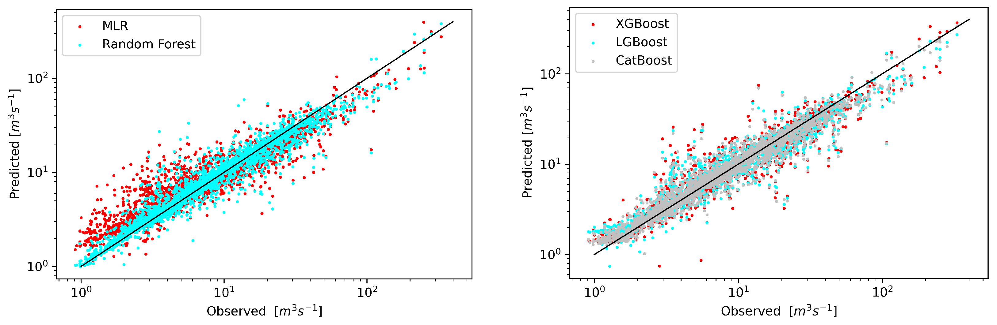
A graphical comparison of the forecast results with the observations for the test data is shown in Figure 3. Benchmark models are characterized by a slightly larger spread of values, especially in the area of low flows.
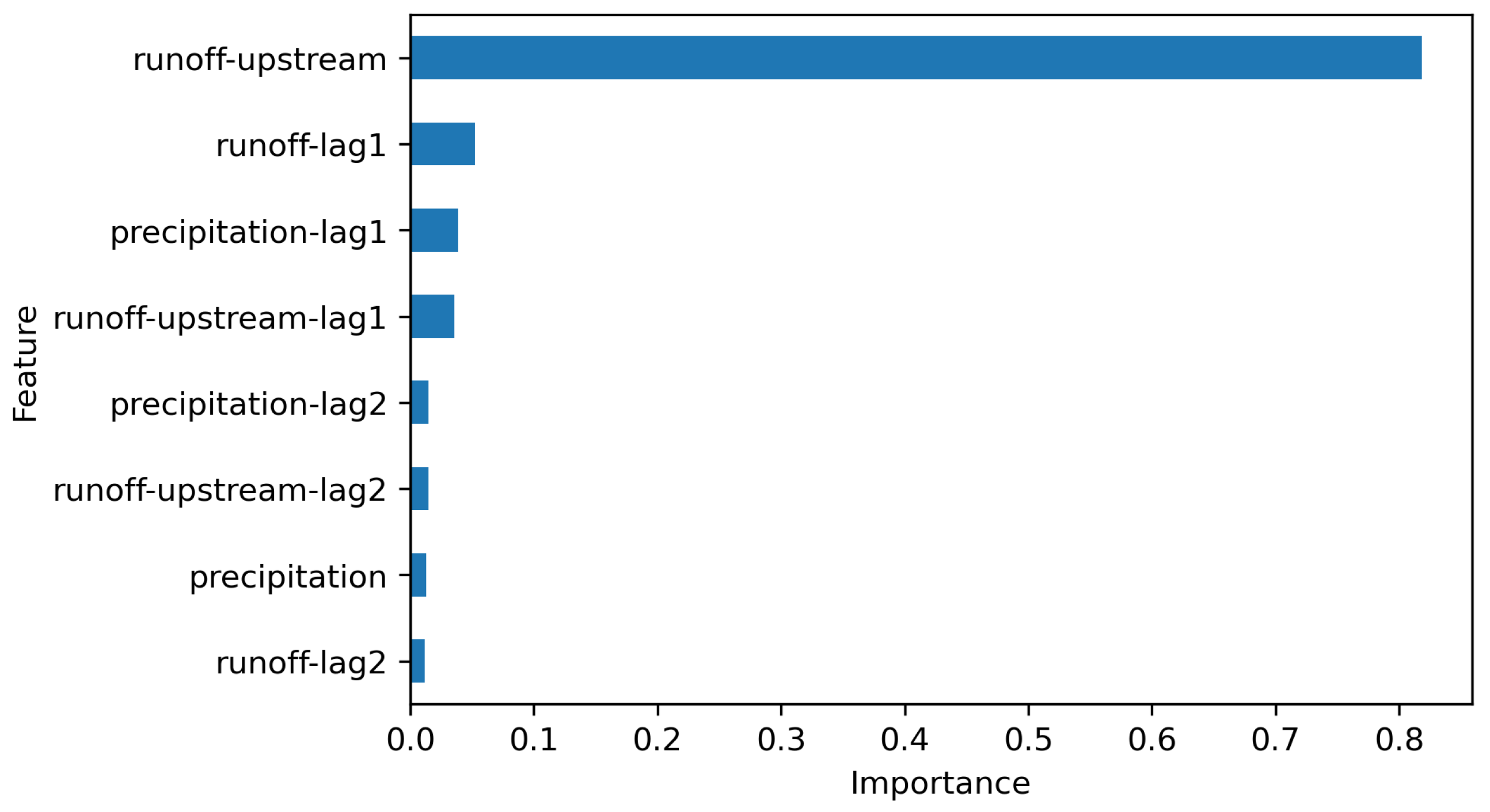
Predictor significance analysis is one of the big advantages of the presented models over the deep learning models. The most important predictor turned out to be the runoff in the upstream cross-section (Osielec) (Figure 4). Other significant features were the information from the previous day: runoff in the tested cross-section, precipitation and runoff in the upstream cross-section.
Table 3 shows the results of the individual models after the optimization of the hyperparameters. The differences between the individual models are slight, although the best results were obtained for the LGBoost model. The resulting NSE is 0.886 and the RMSE is 6.785 ms.
Regardless of the model, these statistics are constant for a wide range of parameter n_estimators and similar learning_rate.
4. Discussion
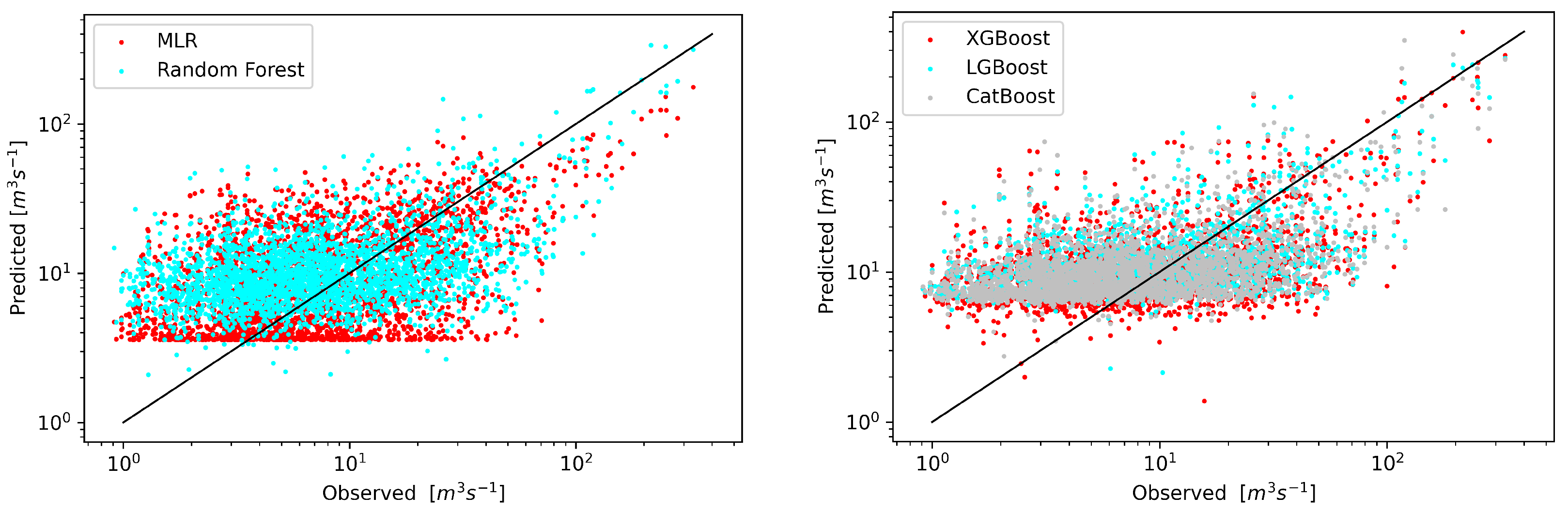
In the first of the analyzed scenarios, the streamflow predictive models would be given only precipitation as input (Figure 5). Given the complexity of such rainfall-runoff models and the relatively low resolution of the precipitation field from the ERA5 project in relation to the size of the catchment area, the poor results visible on the scatterplot should not be surprising. The range of predicted streamflows for each of the models used is much smaller than the range of observed data. Paradoxically, for this data set, the best results were obtained using the reference model—RF. The CatBoost model was the worst. It can be concluded that for this catchment basing only on the precipitation does not give satisfactory results of streamflow forecasts.
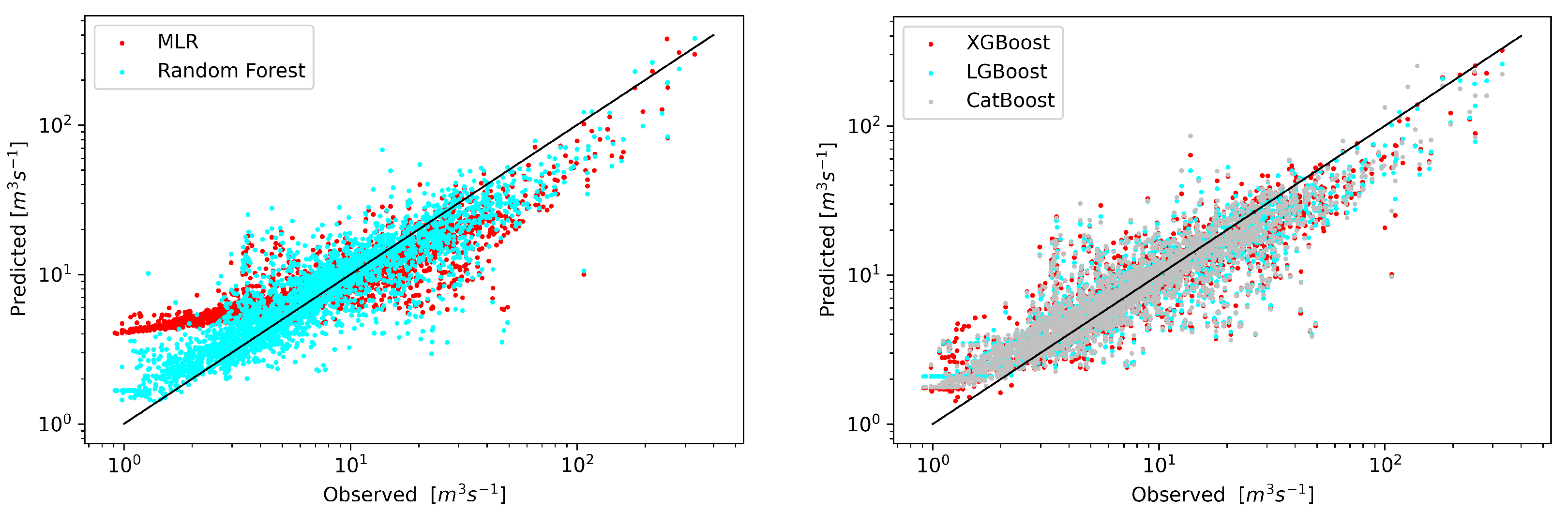
In the second scenario, only the upstream runoff data from the Osielec cross-section was used. The Figure 6 shows a significant improvement, except for the MLR model, which significantly increases the values for low flows. This is consistent with the observation of [52] that XGBoost outperforms SVM model not only in forecasting low flows, but also in high flows in terms of MARE, NSE and R.
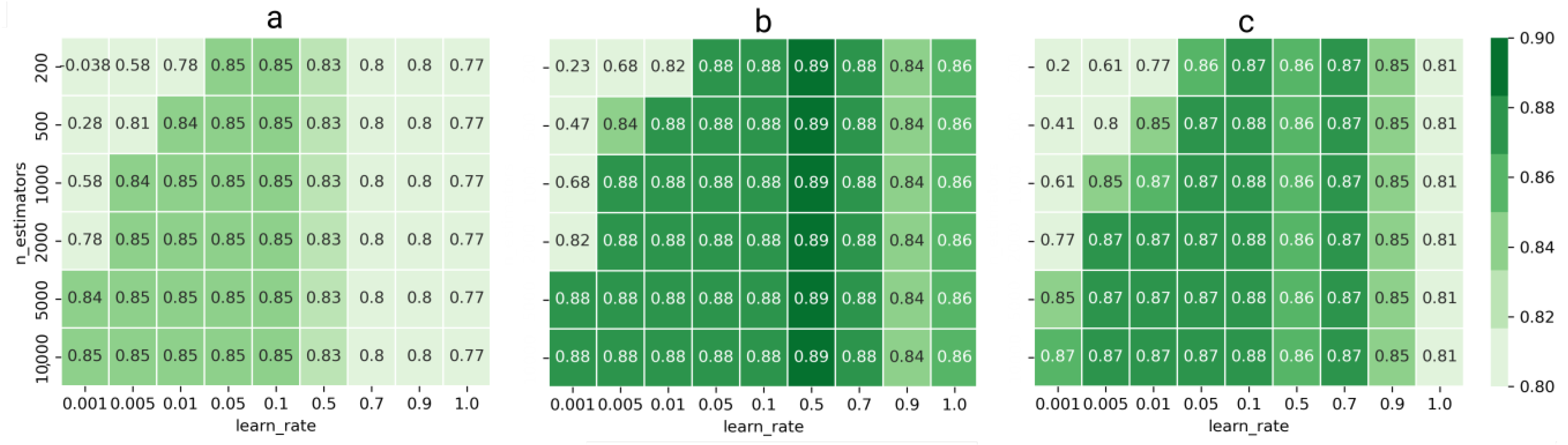
In the last stage of the analysis, optimization of hyperparameters was carried out. Selection of the appropriate hyperparameters of by grid-search and cross validation is time-consuming process [52]. As practice shows, with such a large number of parameters as in the XGBoost model, it may turn out that the obtained results are worse than those generated using the default parameters. It is clearly visible on the attached heatmaps (Figure 7), where for certain combinations of parameters the results are significantly worse than the results before optimization.
As shown by the analysis of hyperparameters (Figure 7), learning rate turned out to be key in optimization. The change in the number of estimators, although having an impact, was not the key optimization direction. Other authors confirm potential problems with the optimization of the XGBoost model, related to the large number of parameters requiring optimization. Ref [52] notes that although the XGBoost shows better capability to deal with overfitting problems than other tree-based models, the hyper-parameters in XGBoost need to be carefully tuned to attain satisfactory forecasts and better generalization capability. The analysis of Figure 7 shows that much more important than the selection of the model is its proper tuning. The differences between the best model results are much smaller than the differences within the models themselves when the wrong parameters are used. When time cannot be spent optimizing hyperparameters, the use of the default regressor parameters may be a better solution to the regression problem for predicting streamflows.
Compared to similar analyzes, we managed to obtain slightly better forecast results. The reason may be a very long time series used for training, consisting of 29 years of daily observations. It was successful despite the use of only a few simple characteristics (precipitation and runoff) with historical data going back only two days. All our tested models achieved NSE in the range of 0.85–0.89 and RMSE in the range of 6.8–7.8 ms.
In [17] study the LSTM model achieved NSE equal 0.68 for daily streamflow prediction based on precipitation, temperature, dew point, wind speed and potential evapotranspiration. Ref [52] for monthly streamflow forecast using XGBoost in two Chinese rivers reported NSE equal about 0.78. For forecast based only on meteorological data using XGBoost [18] achieved NSE of 0.67 and 0.61. [53] reported for deep learning models of monthly streamflow forecast NSE equal 0.75 and 0.76, for CNN and LSTM respectively. Ref [27] compared EA-LSTM with XGBoost, achieving much better results using LSTM for nine years of training data and 531 catchments in US. The meadian NSE score for XGBoost was 0.66, while for LSTM 0.74. Most authors use the oldest and most popular XGBoost model, but our analysis shows that this model is the worst at predicting daily streamflows in mountainous catchments.
An analysis of the hydrographs predicted by individual models can provide many interesting observations, since the model success metrics only provide aggregate statistics. The following paragraphs are devoted to the analysis of selected hydrographs for the test data from years 2010–2017. Due to the high dynamics of streamflows in this catchment, all of the presented graphs show hydrographs in logarithmic scale, as it will make it much easier to see the differences between the models.
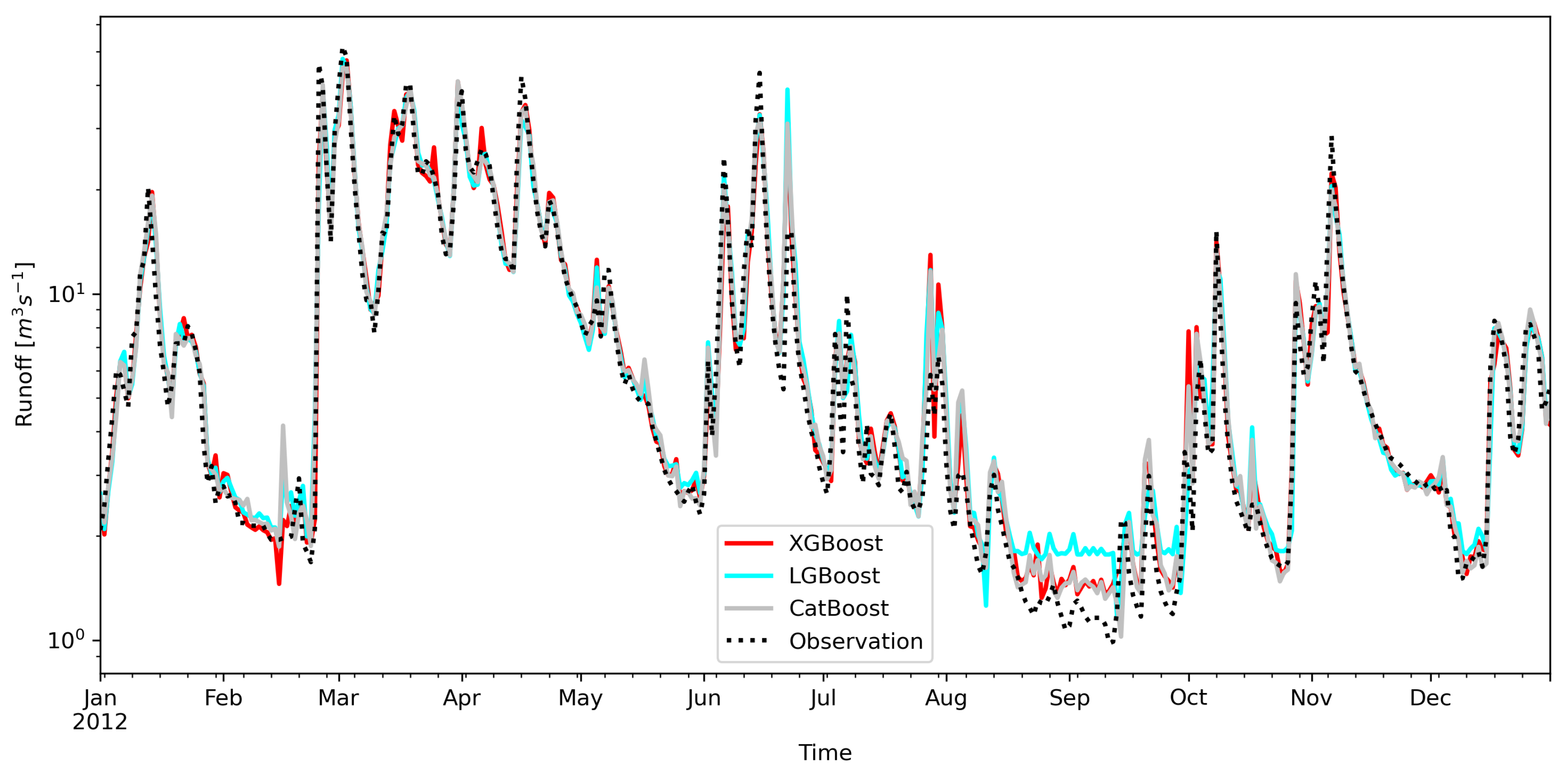
Low flows are usually overestimated for all the models. The LGBoost predictions are the highest and stand out from other models and observations. This is clearly visible at the turn of August and September 2012 (Figure 8). This is not the only such case, so it can be concluded that models of this type are not suitable for forecasting low flows.
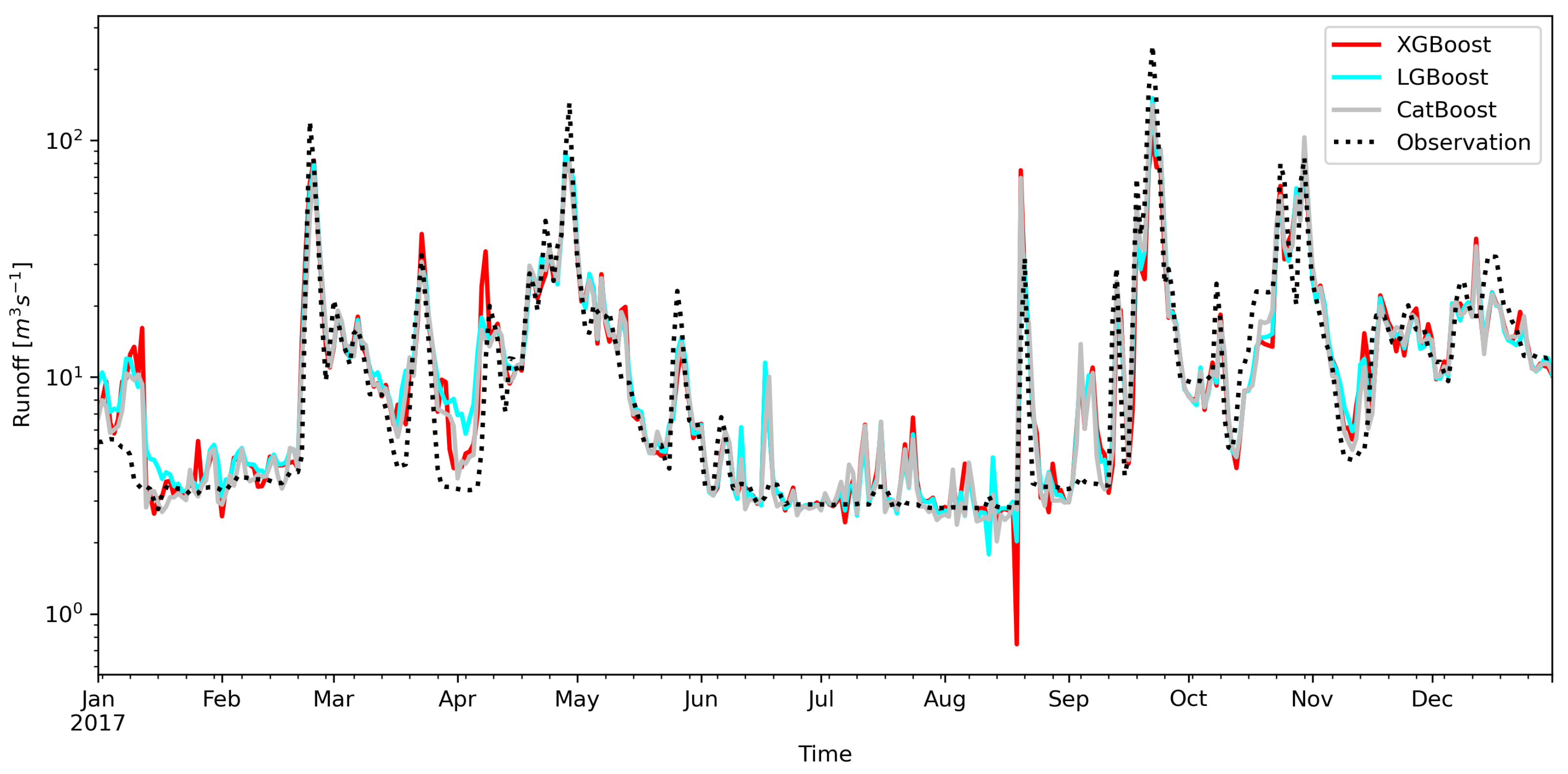
High flows are usually underestimated by all models. With the XGBoost model, the greatest deviations from the observations can be noticed. The tested models have similar problems with mapping some events, e.g., the beginning and middle of 2017 (Figure 9). For unknown reasons, the flow predicted by XGBoost is overestimated here for high flows and underestimated for low flows. The middle of August 2017 is particularly interesting, where the XGBoost forecast is very different from the other models.
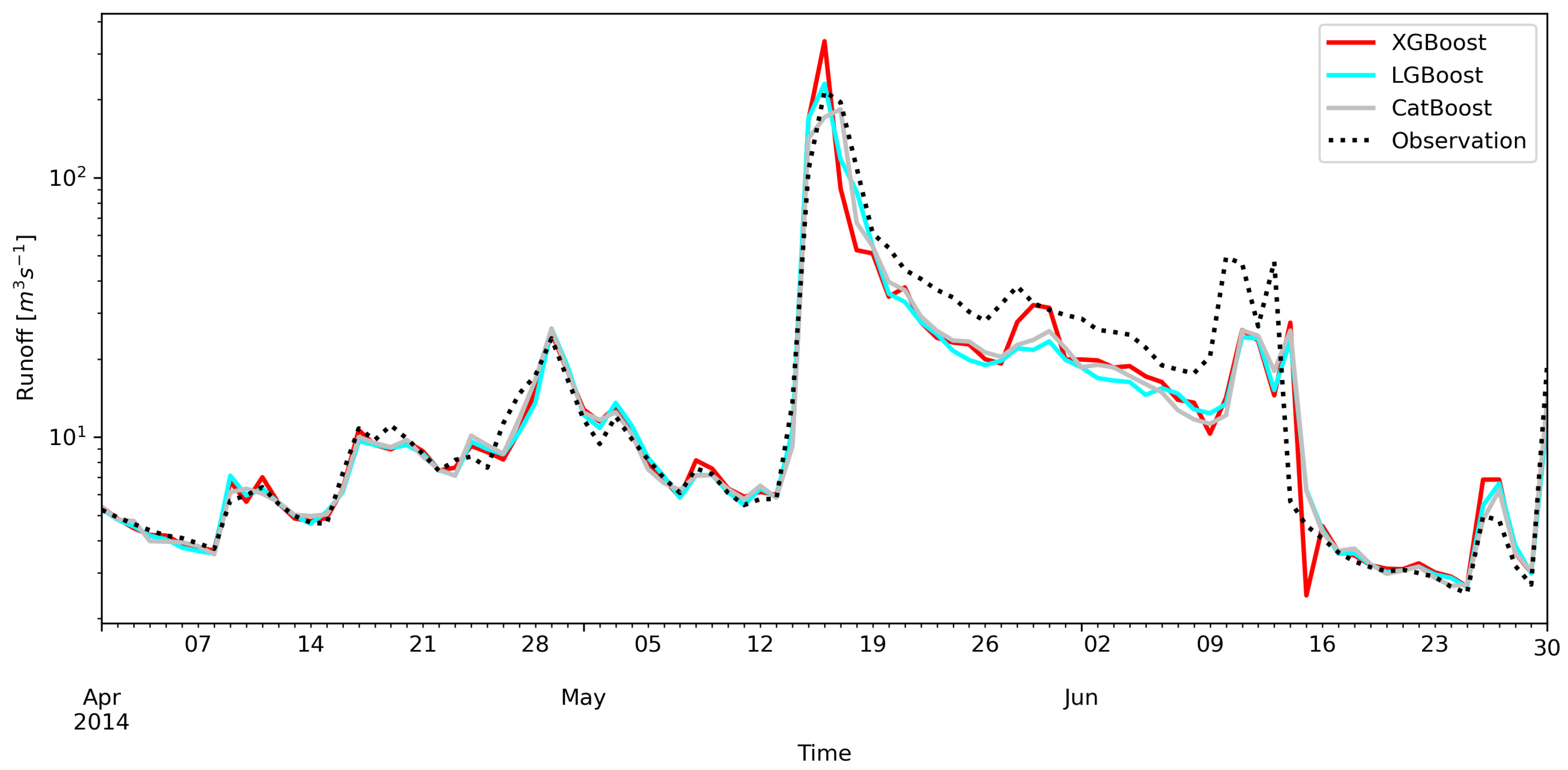
The models usually behave similarly, but there is a difference in the XGBoost forecasts (Figure 10). The plot shows one of the largest flood waves from 2014. The XGBoost model significantly overestimated the flow forecast compared to the other models. You can also see serious problems of all models with the projection of the forecast after the culmination of the wave has passed.
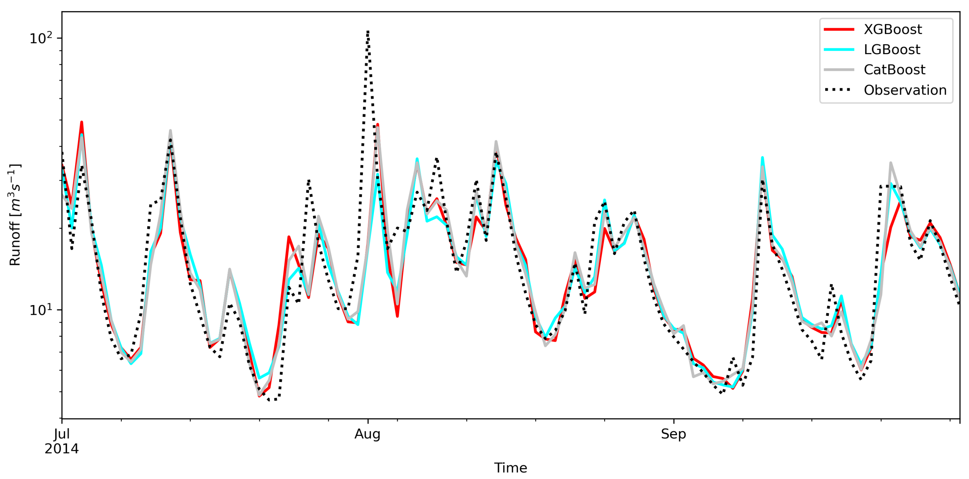
Usually the wave peak time is well predicted, but there are episodes where all models have problems. On average flows from the summer of 2014, individual models generate forecasts that differ from the observational data (Figure 11). The individual waves will appear, but they are shifted in time. The forecasted rising wave from the end of July has completely different dynamics than the observed wave.
It should be noted that the summer period is in Skawa River catchment the time of the most intense precipitation, often with a small spatial extent but high intensity. In this particular period, when precipitation data with sufficiently high spatial resolution is not available, all forecasts are burdened with a considerable error.
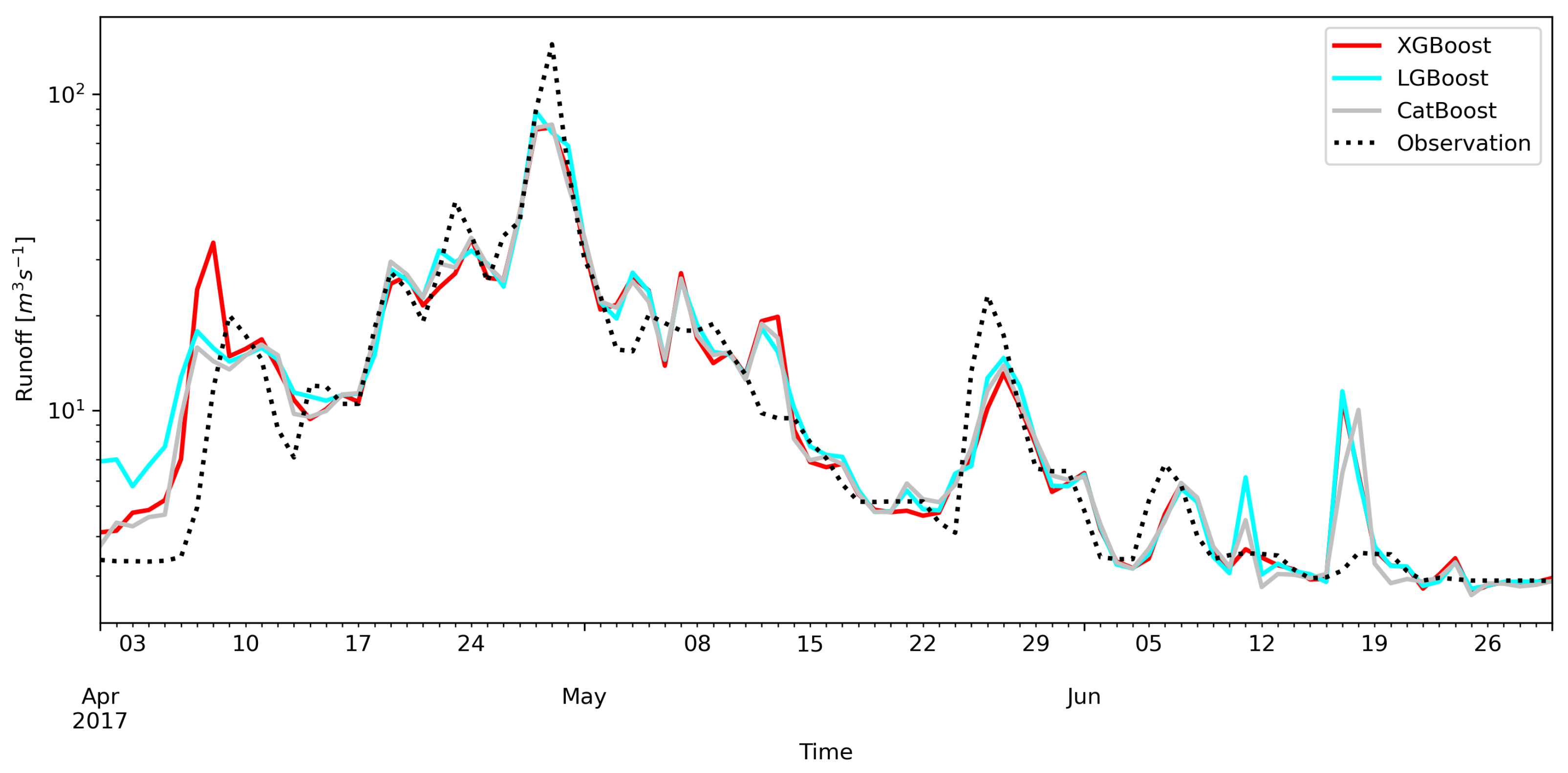
Sometimes the models give the signal of the flood wave in advance of the observation. This can be seen, for example, in the wave from the beginning of April 2017 (Figure 12). It is not easy to explain. This may be due to the fact that the models do not take into account factors such as the catchment retention, which is important in the spring. This may also explain the wave forecast in mid-June 2017 (Figure 12), while water probably from the rainfall may have infiltrated. The analyzed models also lack information about the air temperature and snow cover melting, which is usually used for forecasts. In the analyzed mountain area, water retention in the snow cover affects the water balance in winter and spring.
In the presented analysis, only the most important predictors of streamflow were taken into account. Their selection can be examined in detail thanks to the fact that all of the tested models belong to the Explainable Artificial Intelligence category [54]. This factor determines the advantage of models such as XGBoost, LGBoost or CatBoost over recursive models of the LSTM type, which give slightly better forecasts, but still are difficult to interpret due to their black-box nature.
The feature importance ranking showed in our case that the key information is data on streamflows at the Osielec cross-section located 34 km upstream from Wadowice. Adding information from the last two days on precipitation and streamflows made it possible to obtain results that were slightly better than other authors who used the XGBoost model. Wang et al. [55] identified precipitation as the most important feature, but they did not completely use runoff data as input data. Our forecasts, apart from using the flows on the upstream cross-sections, were probably also possible thanks to the very long measurement series used to learn the model.
For three years of training data (Figure 13) NSE is in the range between 0.60 and 0.74 for LGBoost and XGBoost respectively. For the CatBoost and LGBoost models, you can see a significant and consistent improvement in performance, with NSE approaching 0.90. The XGBoost model is the fastest to get good results, but beyond five years of training data, its NSE is virtually unchanged. We can clearly see the deterioration of the performance of all models at 10 years and then a significant deterioration of the performance of the LGBoost model at 19 years of data. This means that the models, and LGBoost in particular, are sensitive to training data. After exceeding 12 years of training data, the models behave relatively stable. It can therefore be assumed that in the case of such forecasts, this would be the recommended minimum period for model training.
5. Conclusions
Streamflow forecasting is and will continue to be one of the important hydrological tasks. Machine learning models are increasingly used for such predictions. A direct comparison of the use of the three main gradient boosting models (XGBoost, LightGBM and CatBoost) to forecast daily streamflow is our main contribution. We present models performance comparison for mountainous Skawa River catchment, Poland. For this research we use daily precipitation and runoff data from 1981–2017. The conclusions of the analysis are as follows:
- 1.
- The gradient boosting algorithms used in models such as XGBoost, LightGBM and CatBoost are simple to implement, fast and robust. Compared to deep machine learning models (eg LSTM), they allow for easy interpretation of the significance of predictors.
- 2.
- The gradient boosting algorithms provide a good streamflow prediction in mountainous rivers. All tested models achieved Nash-Sutcliffe model efficiency (NSE) in the range of 0.85–0.89 and RMSE in the range of 6.8–7.8 ms.
- 3.
- In order to obtain an NSE above 0.8, the recommended period of training data should be not less than 12 years.
- 4.
- The XGBoost did not turn out to be the best model for the daily flow forecast, although it is the most used model. Assuming the use of models with their default parameters, the best results were obtained with CatBoost. By optimizing the hyperparameters, the best forecast results were obtained by LightGBM.
- 5.
- The differences between the model results are much smaller than the differences within the models themselves when suboptimal hyperparameters are used.
- 6.
- The predictions of the lowest streamflows are overestimated by all analyzed models.
Funding
This research received no external funding.
Data Availability Statement
The runoff data is provided by The Global Runoff Data Centre, 56068 Koblenz, Germany. The precipitation data is provided by Copernicus Climate Change Service Information as ERA-5 Land. Neither the European Commission nor ECMWF is responsible for any use that may be made of the Copernicus Information or Data it contains.
Conflicts of Interest
The authors declare no conflict of interest.
References
- Sit, M.; Demiray, B.Z.; Xiang, Z.; Ewing, G.J.; Sermet, Y.; Demir, I. A comprehensive review of deep learning applications in hydrology and water resources. Water Sci. Technol. 2020, 82, 2635–2670. [Google Scholar] [CrossRef] [PubMed]
- Laimighofer, J.; Melcher, M.; Laaha, G. Low flow estimation beyond the mean–expectile loss and extreme gradient boosting for spatio-temporal low flow prediction in Austria. Hydrol. Earth Syst. Sci. Discuss. 2022, 26, 4553–4574. [Google Scholar] [CrossRef]
- Agana, N.A.; Homaifar, A. EMD-based predictive deep belief network for time series prediction: An application to drought forecasting. Hydrology 2018, 5, 18. [Google Scholar] [CrossRef] [Green Version]
- Sivapragasam, C.; Liong, S.Y. Flow categorization model for improving forecasting. Hydrol. Res. 2005, 36, 37–48. [Google Scholar] [CrossRef]
- Adnan, R.M.; Liang, Z.; Heddam, S.; Zounemat-Kermani, M.; Kisi, O.; Li, B. Least square support vector machine and multivariate adaptive regression splines for streamflow prediction in mountainous basin using hydro-meteorological data as inputs. J. Hydrol. 2020, 586, 124371. [Google Scholar] [CrossRef]
- Stoffel, M.; Wyżga, B.; Marston, R.A. Floods in mountain environments: A synthesis. Geomorphology 2016, 272, 1–9. [Google Scholar] [CrossRef]
- Abdul Kareem, B.; Zubaidi, S.L.; Ridha, H.M.; Al-Ansari, N.; Al-Bdairi, N.S.S. Applicability of ANN Model and CPSOCGSA Algorithm for Multi-Time Step Ahead River Streamflow Forecasting. Hydrology 2022, 9, 171. [Google Scholar] [CrossRef]
- Tyralis, H.; Papacharalampous, G.; Langousis, A. A brief review of random forests for water scientists and practitioners and their recent history in water resources. Water 2019, 11, 910. [Google Scholar] [CrossRef] [Green Version]
- Gauch, M.; Mai, J.; Gharari, S.; Lin, J. Data-driven vs. physically-based streamflow prediction models. In Proceedings of the 9th International Workshop on Climate Informatics, Paris, France, 2–4 October 2019. [Google Scholar]
- Xu, W.; Jiang, Y.; Zhang, X.; Li, Y.; Zhang, R.; Fu, G. Using long short-term memory networks for river flow prediction. Hydrol. Res. 2020, 51, 1358–1376. [Google Scholar] [CrossRef]
- Zealand, C.M.; Burn, D.H.; Simonovic, S.P. Short term streamflow forecasting using artificial neural networks. J. Hydrol. 1999, 214, 32–48. [Google Scholar] [CrossRef]
- Fleming, S.W.; Vesselinov, V.V.; Goodbody, A.G. Augmenting geophysical interpretation of data-driven operational water supply forecast modeling for a western US river using a hybrid machine learning approach. J. Hydrol. 2021, 597, 126327. [Google Scholar] [CrossRef]
- Başağaoğlu, H.; Chakraborty, D.; Lago, C.D.; Gutierrez, L.; Şahinli, M.A.; Giacomoni, M.; Furl, C.; Mirchi, A.; Moriasi, D.; Şengör, S.S. A Review on Interpretable and Explainable Artificial Intelligence in Hydroclimatic Applications. Water 2022, 14, 1230. [Google Scholar] [CrossRef]
- Jose, D.M.; Vincent, A.M.; Dwarakish, G.S. Improving multiple model ensemble predictions of daily precipitation and temperature through machine learning techniques. Sci. Rep. 2022, 12, 4678. [Google Scholar] [CrossRef]
- Cai, Y.; Zheng, W.; Zhang, X.; Zhangzhong, L.; Xue, X. Research on soil moisture prediction model based on deep learning. PLoS ONE 2019, 14, e0214508. [Google Scholar] [CrossRef]
- Zounemat-Kermani, M.; Batelaan, O.; Fadaee, M.; Hinkelmann, R. Ensemble machine learning paradigms in hydrology: A review. J. Hydrol. 2021, 598, 126266. [Google Scholar] [CrossRef]
- Choi, J.; Won, J.; Jang, S.; Kim, S. Learning Enhancement Method of Long Short-Term Memory Network and Its Applicability in Hydrological Time Series Prediction. Water 2022, 14, 2910. [Google Scholar] [CrossRef]
- Afshari, M. Using LSTM and XGBoost for Streamflow Prediction Based on Meteorological Time Series Data. Master’s Thesis, Utrecht University, Utrecht, The Netherlands, 2022. [Google Scholar]
- Liu, J.; Ren, K.; Ming, T.; Qu, J.; Guo, W.; Li, H. Investigating the effects of local weather, streamflow lag, and global climate information on 1-month-ahead streamflow forecasting by using XGBoost and SHAP: Two case studies involving the contiguous USA. Acta Geophys. 2022, 1–21. [Google Scholar] [CrossRef]
- Lundberg, S.M.; Lee, S.I. A unified approach to interpreting model predictions. In Proceedings of the Advances in Neural Information Processing Systems, Long Beach, CA, USA, 4–9 December 2017; Volume 30. [Google Scholar]
- Choubin, B.; Khalighi-Sigaroodi, S.; Malekian, A.; Kişi, Ö. Multiple linear regression, multi-layer perceptron network and adaptive neuro-fuzzy inference system for forecasting precipitation based on large-scale climate signals. Hydrol. Sci. J. 2016, 61, 1001–1009. [Google Scholar] [CrossRef]
- Abed, M.; Imteaz, M.A.; Ahmed, A.N.; Huang, Y.F. Modelling monthly pan evaporation utilising Random Forest and deep learning algorithms. Sci. Rep. 2022, 12, 13132. [Google Scholar] [CrossRef]
- Papacharalampous, G.A.; Tyralis, H. Evaluation of random forests and Prophet for daily streamflow forecasting. Adv. Geosci. 2018, 45, 201–208. [Google Scholar] [CrossRef]
- Bhusal, A.; Parajuli, U.; Regmi, S.; Kalra, A. Application of Machine Learning and Process-Based Models for Rainfall-Runoff Simulation in DuPage River Basin, Illinois. Hydrology 2022, 9, 117. [Google Scholar] [CrossRef]
- Graf, R.; Kolerski, T.; Zhu, S. Predicting Ice Phenomena in a River Using the Artificial Neural Network and Extreme Gradient Boosting. Resources 2022, 11, 12. [Google Scholar] [CrossRef]
- Weierbach, H.; Lima, A.R.; Willard, J.D.; Hendrix, V.C.; Christianson, D.S.; Lubich, M.; Varadharajan, C. Stream temperature predictions for river basin management in the Pacific Northwest and mid-Atlantic regions using machine learning. Water 2022, 14, 1032. [Google Scholar] [CrossRef]
- Gauch, M.; Mai, J.; Lin, J. The proper care and feeding of CAMELS: How limited training data affects streamflow prediction. Environ. Model. Softw. 2021, 135, 104926. [Google Scholar] [CrossRef]
- van den Munckhof, G. Forecasting River Discharge Using Machine Learning Methods. Master’s Thesis, Delft University of Technology, Delft, The Netherlands, 2020. [Google Scholar]
- Tyralis, H.; Papacharalampous, G.; Langousis, A. Super ensemble learning for daily streamflow forecasting: Large-scale demonstration and comparison with multiple machine learning algorithms. Neural Comput. Appl. 2021, 33, 3053–3068. [Google Scholar] [CrossRef]
- Ke, G.; Meng, Q.; Finley, T.; Wang, T.; Chen, W.; Ma, W.; Ye, Q.; Liu, T.Y. LightGBM: A Highly Efficient Gradient Boosting Decision Tree. In Proceedings of the Advances in Neural Information Processing Systems, Long Beach, CA, USA, 4–9 December 2017; Guyon, I., Luxburg, U.V., Bengio, S., Wallach, H., Fergus, R., Vishwanathan, S., Garnett, R., Eds.; Curran Associates, Inc.: Red Hook, NY, USA, 2017; Volume 30. [Google Scholar]
- Prokhorenkova, L.; Gusev, G.; Vorobev, A.; Dorogush, A.V.; Gulin, A. CatBoost: Unbiased boosting with categorical features. In Proceedings of the Advances in Neural Information Processing Systems, Montreal, QC, USA, 3–8 December 2018; Volume 31. [Google Scholar]
- Dorogush, A.V.; Ershov, V.; Gulin, A. CatBoost: Gradient boosting with categorical features support. arXiv 2018, arXiv:1810.11363. [Google Scholar]
- Hancock, J.T.; Khoshgoftaar, T.M. CatBoost for big data: An interdisciplinary review. J. Big Data 2020, 7, 94. [Google Scholar] [CrossRef]
- Muñoz-Sabater, J.; Dutra, E.; Agustí-Panareda, A.; Albergel, C.; Arduini, G.; Balsamo, G.; Boussetta, S.; Choulga, M.; Harrigan, S.; Hersbach, H.; et al. ERA5-Land: A state-of-the-art global reanalysis dataset for land applications. Earth Syst. Sci. Data 2021, 13, 4349–4383. [Google Scholar] [CrossRef]
- Papacharalampous, G.; Tyralis, H. Time series features for supporting hydrometeorological explorations and predictions in ungauged locations using large datasets. Water 2022, 14, 1657. [Google Scholar] [CrossRef]
- Bokwa, A.; Klimek, M.; Krzaklewski, P.; Kukułka, W. Drought Trends in the Polish Carpathian Mts. in the Years 1991–2020. Atmosphere 2021, 12, 1259. [Google Scholar] [CrossRef]
- Baran-Gurgul, K. The Risk of Extreme Streamflow Drought in the Polish Carpathians—A Two-Dimensional Approach. Int. J. Environ. Res. Public Health 2022, 19, 14095. [Google Scholar] [CrossRef]
- Kędra, M. Altered precipitation characteristics in two Polish Carpathian basins, with implications for water resources. Clim. Res. 2017, 72, 251–265. [Google Scholar] [CrossRef]
- Twardosz, R.; Cebulska, M.; Walanus, A. Anomalously heavy monthly and seasonal precipitation in the Polish Carpathian Mountains and their foreland during the years 1881–2010. Theor. Appl. Climatol. 2016, 126, 323–337. [Google Scholar] [CrossRef] [Green Version]
- Kholiavchuk, D.; Cebulska, M. The highest monthly precipitation in the area of the Ukrainian and the Polish Carpathian Mountains in the period from 1984 to 2013. Theor. Appl. Climatol. 2019, 138, 1615–1628. [Google Scholar] [CrossRef]
- Falarz, M.; Bednorz, E. Snow cover change. In Climate Change in Poland; Springer: Berlin/Heidelberg, Germany, 2021; pp. 375–390. [Google Scholar] [CrossRef]
- Wyżga, B. Impact of the channelization-induced incision of the Skawa and Wisłoka Rivers, southern Poland, on the conditions of overbank deposition. Regul. Rivers Res. Manag. Int. J. Devoted River Res. Manag. 2001, 17, 85–100. [Google Scholar] [CrossRef]
- Olive, D.J. Multiple Linear Regression; Springer: Berlin/Heidelberg, Germany, 2017. [Google Scholar] [CrossRef]
- Svetnik, V.; Liaw, A.; Tong, C.; Culberson, J.C.; Sheridan, R.P.; Feuston, B.P. Random forest: A classification and regression tool for compound classification and QSAR modeling. J. Chem. Inf. Comput. Sci. 2003, 43, 1947–1958. [Google Scholar] [CrossRef]
- Chen, T.; Guestrin, C. Xgboost: A scalable tree boosting system. In Proceedings of the 22nd ACM SIGKDD International Conference on Knowledge Discovery and Data Mining, San Francisco, CA, USA, 13–17 August 2016; pp. 785–794. [Google Scholar] [CrossRef] [Green Version]
- Rao, H.; Shi, X.; Rodrigue, A.K.; Feng, J.; Xia, Y.; Elhoseny, M.; Yuan, X.; Gu, L. Feature selection based on artificial bee colony and gradient boosting decision tree. Appl. Soft Comput. 2019, 74, 634–642. [Google Scholar] [CrossRef]
- Gan, M.; Pan, S.; Chen, Y.; Cheng, C.; Pan, H.; Zhu, X. Application of the machine learning lightgbm model to the prediction of the water levels of the lower columbia river. J. Mar. Sci. Eng. 2021, 9, 496. [Google Scholar] [CrossRef]
- Cui, Z.; Qing, X.; Chai, H.; Yang, S.; Zhu, Y.; Wang, F. Real-time rainfall-runoff prediction using light gradient boosting machine coupled with singular spectrum analysis. J. Hydrol. 2021, 603, 127124. [Google Scholar] [CrossRef]
- Pedregosa, F.; Varoquaux, G.; Gramfort, A.; Michel, V.; Thirion, B.; Grisel, O.; Blondel, M.; Prettenhofer, P.; Weiss, R.; Dubourg, V.; et al. Scikit-learn: Machine Learning in Python. J. Mach. Learn. Res. 2011, 12, 2825–2830. [Google Scholar]
- Nash, J.E.; Sutcliffe, J.V. River flow forecasting through conceptual models part I—A discussion of principles. J. Hydrol. 1970, 10, 282–290. [Google Scholar] [CrossRef]
- Moriasi, D.N.; Arnold, J.G.; Van Liew, M.W.; Bingner, R.L.; Harmel, R.D.; Veith, T.L. Model evaluation guidelines for systematic quantification of accuracy in watershed simulations. Trans. ASABE 2007, 50, 885–900. [Google Scholar] [CrossRef]
- Ni, L.; Wang, D.; Wu, J.; Wang, Y.; Tao, Y.; Zhang, J.; Liu, J. Streamflow forecasting using extreme gradient boosting model coupled with Gaussian mixture model. J. Hydrol. 2020, 586, 124901. [Google Scholar] [CrossRef]
- Forghanparast, F.; Mohammadi, G. Using Deep Learning Algorithms for Intermittent Streamflow Prediction in the Headwaters of the Colorado River, Texas. Water 2022, 14, 2972. [Google Scholar] [CrossRef]
- Meddage, D.; Ekanayake, I.; Herath, S.; Gobirahavan, R.; Muttil, N.; Rathnayake, U. Predicting Bulk Average Velocity with Rigid Vegetation in Open Channels Using Tree-Based Machine Learning: A Novel Approach Using Explainable Artificial Intelligence. Sensors 2022, 22, 4398. [Google Scholar] [CrossRef]
- Wang, S.; Peng, H.; Hu, Q.; Jiang, M. Analysis of runoff generation driving factors based on hydrological model and interpretable machine learning method. J. Hydrol. Reg. Stud. 2022, 42, 101139. [Google Scholar] [CrossRef]
Figure 1.
Skawa River catchment (red area) with gauge stations used in presented research—Osielec and Wadowice.
Figure 1.
Skawa River catchment (red area) with gauge stations used in presented research—Osielec and Wadowice.

Figure 2.
Sample data used in presented research—daily precipitation and daily runoff at three cross-sections of Skawa River in summer 1990.
Figure 2.
Sample data used in presented research—daily precipitation and daily runoff at three cross-sections of Skawa River in summer 1990.

Figure 3.
Scatterplot of observed and predicted streamflow with default model parameters for all data scenario (precipitation, upstream and lag runoff).
Figure 3.
Scatterplot of observed and predicted streamflow with default model parameters for all data scenario (precipitation, upstream and lag runoff).

Figure 4.
The XGBoost model built-in feature importance. Lag1 suffix corresponds to information from previous day, lag2 from two days ago. Runoff features are for Wadowice cross-section, while runoff-upstream for Osielec cross-section.
Figure 4.
The XGBoost model built-in feature importance. Lag1 suffix corresponds to information from previous day, lag2 from two days ago. Runoff features are for Wadowice cross-section, while runoff-upstream for Osielec cross-section.

Figure 5.
Forecast with default parameters based only on precipitation data.

Figure 6.
Forecast with default parameters based only on runoff data.

Figure 7.
NSE values in hyperparameters optimization for (a) XGBoost, (b) LGBoost and (c) CatBoost.

Figure 8.
Daily runoff forecast for Wadowice on Skawa River in year 2012—low flows case.

Figure 9.
Daily runoff forecast for Wadowice on Skawa River in year 2017—high flows case.

Figure 10.
Daily runoff forecast for Wadowice on Skawa River—XGBoost performance problems.

Figure 11.
Daily runoff forecast for Wadowice on Skawa River—problem with flood wave peak time.

Figure 12.
Daily runoff forecast for Wadowice on Skawa River—problem with forecast in advance.

Figure 13.
Nash-Sutcliffe model efficiency as function of training dataset legth (years of daily observations).
Figure 13.
Nash-Sutcliffe model efficiency as function of training dataset legth (years of daily observations).


Table 1.
The predictor variables used in subsequent scenarios (indicated by X). Lag1 and lag2 are observations from n antecedent days.
Table 1.
The predictor variables used in subsequent scenarios (indicated by X). Lag1 and lag2 are observations from n antecedent days.
| Predictor | Scenario 1 | Scenario 2 | Scenario 3 |
|---|---|---|---|
| Precipitation | X | X | |
| Precipitation lag1 | X | X | |
| Precipitation lag2 | X | X | |
| Runoff upstream (Osielec) | X | X | |
| Runoff upstream lag1 | X | X | |
| Runoff upstream lag2 | X | X | |
| Runoff lag1 (Wadowice) | X | ||
| Runoff lag2 | X |
Table 2.
Streamflow forecast model performance with default parameters. The best results for each scenario are underlined, the worst are in italic.
Table 2.
Streamflow forecast model performance with default parameters. The best results for each scenario are underlined, the worst are in italic.
| Model | Only Precipitation | Only Upstream Runoff | All Parameters | ||||||
|---|---|---|---|---|---|---|---|---|---|
| NSE | RMSE | MAE | NSE | RMSE | MAE | NSE | RMSE | MAE | |
| MLR | 0.460 | 14.798 | 8.500 | 0.748 | 10.104 | 4.784 | 0.848 | 7.850 | 3.142 |
| RF | 0.533 | 13.765 | 8.385 | 0.773 | 9.595 | 4.073 | 0.848 | 7.841 | 2.606 |
| XGBoost | 0.467 | 14.692 | 8.364 | 0.777 | 9.506 | 3.958 | 0.839 | 8.082 | 2.633 |
| LGBoost | 0.524 | 13.888 | 8.224 | 0.759 | 9.885 | 3.960 | 0.876 | 7.077 | 2.508 |
| CatBoost | 0.436 | 15.120 | 8.343 | 0.739 | 10.274 | 4.041 | 0.886 | 6.800 | 2.400 |
Table 3.
Streamflow forecast model performance after hyperparameters optimization. The best results are underlined, the worst are in italic.
Table 3.
Streamflow forecast model performance after hyperparameters optimization. The best results are underlined, the worst are in italic.
| Model | NSE | RMSE | MAE | n_estimators | learning_rate |
|---|---|---|---|---|---|
| XGBoost | 0.850 | 7.798 | 2.598 | 500–10,000 | 0.1 |
| LGBoost | 0.886 | 6.785 | 2.696 | 200–10,000 | 0.5 |
| CatBoost | 0.878 | 7.024 | 2.462 | 1000–10,000 | 0.1 |
Publisher’s Note: MDPI stays neutral with regard to jurisdictional claims in published maps and institutional affiliations. |
© 2022 by the author. Licensee MDPI, Basel, Switzerland. This article is an open access article distributed under the terms and conditions of the Creative Commons Attribution (CC BY) license (https://creativecommons.org/licenses/by/4.0/).
Share and Cite
MDPI and ACS Style
Szczepanek, R. Daily Streamflow Forecasting in Mountainous Catchment Using XGBoost, LightGBM and CatBoost. Hydrology 2022, 9, 226. https://doi.org/10.3390/hydrology9120226
AMA Style
Szczepanek R. Daily Streamflow Forecasting in Mountainous Catchment Using XGBoost, LightGBM and CatBoost. Hydrology. 2022; 9(12):226. https://doi.org/10.3390/hydrology9120226
Chicago/Turabian StyleSzczepanek, Robert. 2022. "Daily Streamflow Forecasting in Mountainous Catchment Using XGBoost, LightGBM and CatBoost" Hydrology 9, no. 12: 226. https://doi.org/10.3390/hydrology9120226
Note that from the first issue of 2016, this journal uses article numbers instead of page numbers. See further details here.