Article

Monitoring and Quantifying the Fluvio-Geomorphological Changes in a Torrent Channel Using Images from Unmanned Aerial Vehicles

by
Georgios T. Gkiatas
,
Paschalis D. Koutalakis
,
Iordanis K. Kasapidis
,
Valasia Iakovoglou
and
George N. Zaimes
*
Geomorphology Edaphology and Riparian Areas Laboratory (GERi Lab), Department of Forestry and Natural Environment Science, International Hellenic University, 66100 Drama, Greece
*
Author to whom correspondence should be addressed.
Hydrology 2022, 9(10), 184; https://doi.org/10.3390/hydrology9100184
Submission received: 15 September 2022 / Revised: 7 October 2022 / Accepted: 16 October 2022 / Published: 19 October 2022

Abstract

:
The study attempts to monitor geomorphological changes (e.g., erosion/deposition) with innovative tools at a typical Mediterranean torrent. The torrent’s geomorphological conditions are studied for an entire affected stream reach. The investigation utilizes two different environments/point views: (a) traditional terrestrial and (b) innovative aerial. The traditional methods include erosion pins at streambanks and field cross-section measurements of the stream channel. For the innovative methods, utilizing an unmanned aerial vehicle, in order to monitor the geomorphologic changes in the entire reach during different days over the last 3 years (2020–2022), there was a total of six flights. The results from innovative methods showcase the episodic nature of stream channel changes since erosion and deposition were captured during the different monitoring periods. Even during one flight in one cross-section, the stream bed and two banks in many cases experienced different changes. The significant erosion and deposition recorded showcase the disequilibrium in the torrent. In addition, the impact of the anthropogenic structure (Irish bridge) is evident, since upstream, more substantial deposition was recorded compared to downstream. The similarity of the results between the innovative method and the traditional methods indicates the method’s effectiveness and the potential usefulness in using UAV images for stream bank and bed monitoring. One of the biggest advantages is the ability to monitor the entire reach at substantially lower costs and time compared to the traditional methods. Still, more testing needs to be conducted in different stream and river environments to better refine the method in order to be adopted by land and water managers to be used for stream and river monitoring.

1. Introduction

Torrents, typically having ephemeral and intermittent flow, are categorized as low order and are the dominant flowing water body type in semi-arid regions in Europe [1]. The low-order Mediterranean torrents that flow directly into the sea represent about 26% of the total while their area coverage in Greece is even higher, reaching 42.5% of the country’s territory [2]. This percentage increases significantly if we consider the torrents that are tributaries of larger streams or rivers that also end up in the sea.
Stream bank and bed erosion/deposition are major dynamic fluvio-geomorphologic processes. Altering the dynamic equilibrium and base level of the stream or torrent induces changes in the bed and banks, typically causing significant degradation of the riverine ecosystems [3]. In Greece, where the Mediterranean climate prevails, the heavy rainfalls, especially during the wet season, often cause severe flooding and torrential phenomena [4,5]. Even small flood events can have a significant impact on agricultural and urban activities, in urban and natural environments [6,7]. The changes in the stream bed and banks and the sediment transport capacity (volume of transported materials) are of major importance, as they can change the flow path of the channel and cause significant damage to the adjacent infrastructure. In the Mediterranean region, the flash floods are very common [8]. The flash floods are among the most dangerous natural disasters, as they cause rapid flow of water in rivers and streams and cover their surrounding flood zones with water, sediment and debris [9]. The flash floods can transport substantial amounts of sediment, rock and woody vegetation or even entire trees, causing serious problems to human infrastructure [10]. In addition, the sediment yield originating from the erosional and depositional processes along the stream banks play important roles in the non-point source pollution concentration levels of the water resources [11]. The suspended sediment can carry and absorb other pollutants (especially heavy metals, e.g., Cr, Cd, Hg, Cu, Fe, Zn, Pb, As) in the flowing waters of torrents, streams and rivers and deposit them onto the stream bed and banks or on other final recipients (e.g., lake or sea) [12]. Excessive erosion rates, as a consequence of urban and agricultural expansion, deforestation and wildfires, can intensify the sediments’ volumes (increase sediment transport capacity) even in the normally clean-water environments [13]. This can result in increased water pollution, produce negative effects on the fish and even humans through the food chain and degrade the environmental status of the water resource and the adjacent areas [14]. Land use is an influential factor in river sediment pollution [15]. For the above reasons, studying, monitoring and understanding fluvio-geomorphologic processes is a priority, particularly in drylands and semi-arid regions, such as the Mediterranean [16].
To improve the understanding and monitoring of flash floods in torrents and the process of erosion and deposition, several methodologies have been developed and implemented worldwide [17]. One of the most commonly and widely used methods is the Universal Soil Loss Equation (USLE), a soil erosion model that predicts the rate of soil loss based on rainfall, soil type, slope, cropping systems, land cover and control practices [18]. Another method is the Gavrilovic equation, also known as the Erosion Potential Model (EPM), which is an empirical and semi-quantitative method to estimate the amount of sediment transport and erosion intensity [19,20]. The EPM has been extensively applied, since 1968 in Balkan countries, while currently, it is also being applied worldwide [21]. Traditional field methods can be complimentary and help validate the previously mentioned models. The most frequent practices include the placement of erosion pins in the stream banks and stream cross-sections (CSs), which are the cheapest methods among the field methods but are highly demanding in regard to time and personnel effort [22,23]. Other methods for recording and indicating geomorphological changes include traditional runoff graphs [24], data acquisition systems with telemetry logger, ultrasonic signal erosion tools [25,26], recordings and comparisons with cameras [27], ground terrain scanners and topographic studies using a total station [28] as well as remote sensing tools using unmanned aerial vehicles (UAVs) [29]. UAV applications have grown rapidly over the past decade and their utilization is accelerating for disaster management, such as floods, erosion, earthquakes/landslides and wildfires [30,31,32]. The UAV products (e.g., 3D models and orthophoto maps) can be applied to study and monitor the natural disasters and, thus, are becoming a necessity for all studies, which are related to damage identification by aerial monitoring [33].
There is still a scientific need to better understand the temporal and spatial characteristics of fluvio-geomorphological processes. The methodology’s measurement time interval is one of the most critical elements [34]. Remote sensing, extensively utilizing satellite and UAV images, has become an important tool for fluvial geomorphology monitoring [35,36]. The costs of images acquisition, the weather conditions and the vegetation cover of the studied area are limitations that must be considered when using these tools [37,38]. Capturing images of the torrent channel at different periods with successive UAV flights allows one to identify changes along the channel banks and bed and, in many cases, can lead to the quantitative determination of the sediment deposited or eroded in the bank and/or channel [39]. The main advantages of utilizing UAVs are the reduced time and cost and the enhanced data acquisition and image resolution, compared to terrestrial photogrammetry and satellite remote sensing systems [40]. The main concerns of UAVs are not being able to fly under extreme weather conditions (e.g., high-wind conditions) and the battery flight time limitation [41]. Still, the ability to fly after major fluvio-geomorphologic events (e.g., floods) provides images at the needed temporal and spatial scale that showcase the impacts of these events.
Utilizing UAVs is becoming an accepted methodology to capture the characteristics of an area of interest and create detailed orthophotos [42]. It is also combined and compared to other fluvio-geomorphologic survey tools, such as repeated sampling, including erosion pins [43] or photo-electric erosion pins to monitor the stream bank changes [44] or by performing GNSS topographic surveys or helicopter-based full-waveform LiDAR [45]. Studies have also investigated the strengths and weaknesses of direct sediment observations of river-channel morphology, while analyzing the uncertainty in sediment volume estimates by comparing digital surface models (DSMs) between flood events [46,47,48]. Monitoring DSM differences to quantify the elevation change rates at the ground surface, which comprise erosion, accretion and sedimentation, has been implemented. The limitation of this technique is the presence of vegetation presence in the datasets, although there are efforts that develop algorithms able to estimate the elevation height underneath the vegetation canopy [49]. These datasets proved to be capable of providing high resolution to quantify intra- and multiannual sediment changes and riverbed patterns [50]. Recently, UAVs have been applied in ungauged gullies and torrents to capture the debris flow and monitor erosion and deposition events [51,52,53]. In addition, UAV-based surveys performed to support restoration activities and propose the design of effective measures to mitigate severe effects [54]. Finally, De Haas et al. studied the spatio-temporal patterns of erosion and deposition in debris-flow torrents and showcased that they are highly variable and dynamic while the check dams strongly control the spatial patterns of erosion and deposition and can provide key guidelines for flow volume forecasting [55].
This specific study focuses on the application of modern methods (from an aerial point of view) to capture, map and provide quantitative measures of fluvio-geomorphological changes in the Kallifitos torrent in the area of Drama, Greece. In addition, the modern methods are compared to traditional methods (from a terrestrial point of view) to validate the results. The proposed methodology can be a reliable tool for responsible authorities, to monitor fluvio-geomorphologic changes in torrents and help in targeted mitigation efforts to be applied to the most dominant type of watercourse in the Mediterranean region. Torrent flash flooding in the Mediterranean, as a result of the acceleration of the hydrologic cycle due to climate change and the expansion of urban areas in the floodplains, is one of the main disasters of concern, especially in urban settings [7].

2. Materials and Methods

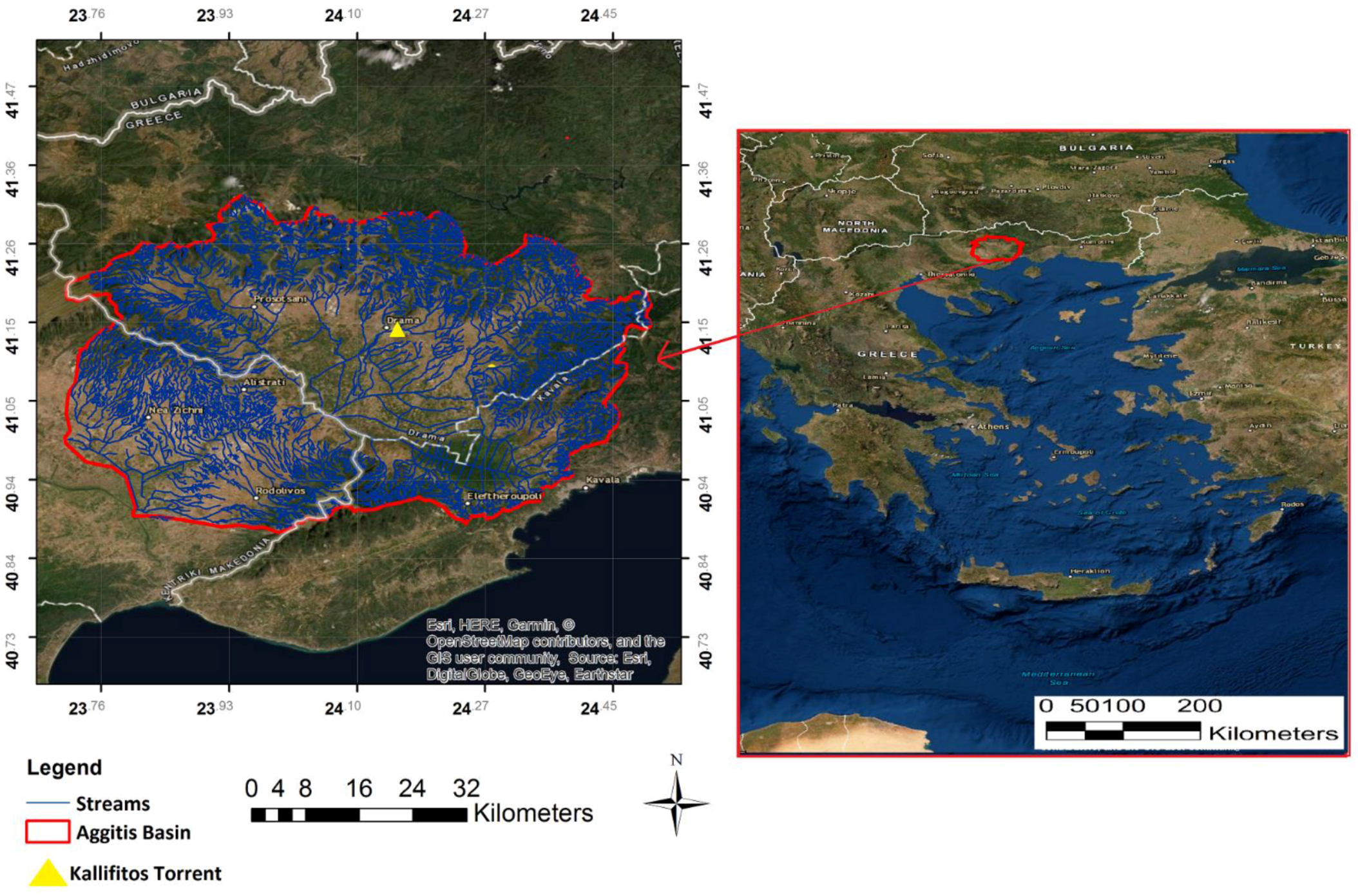
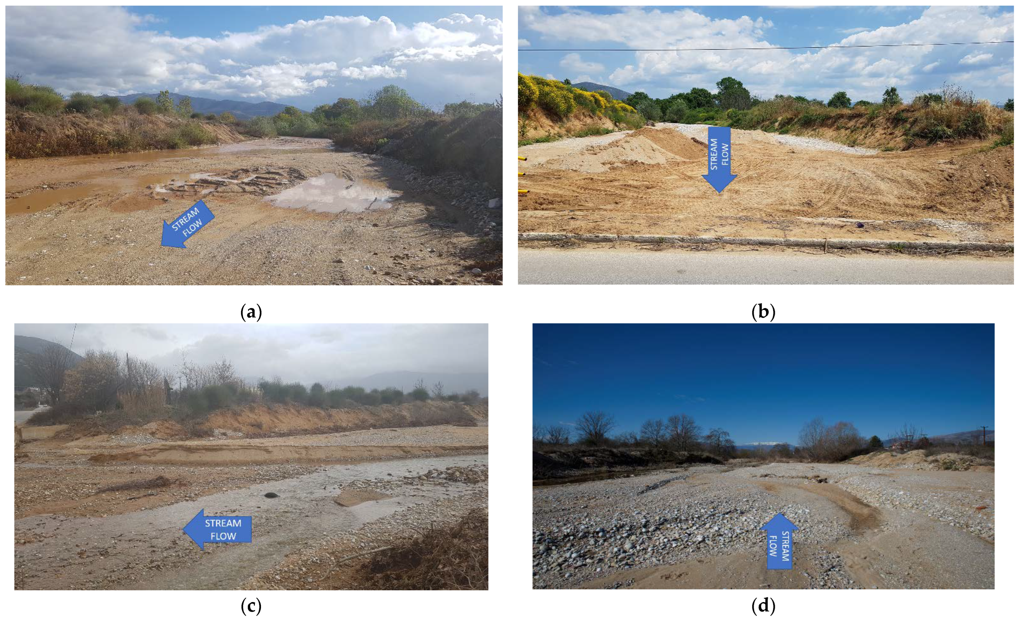
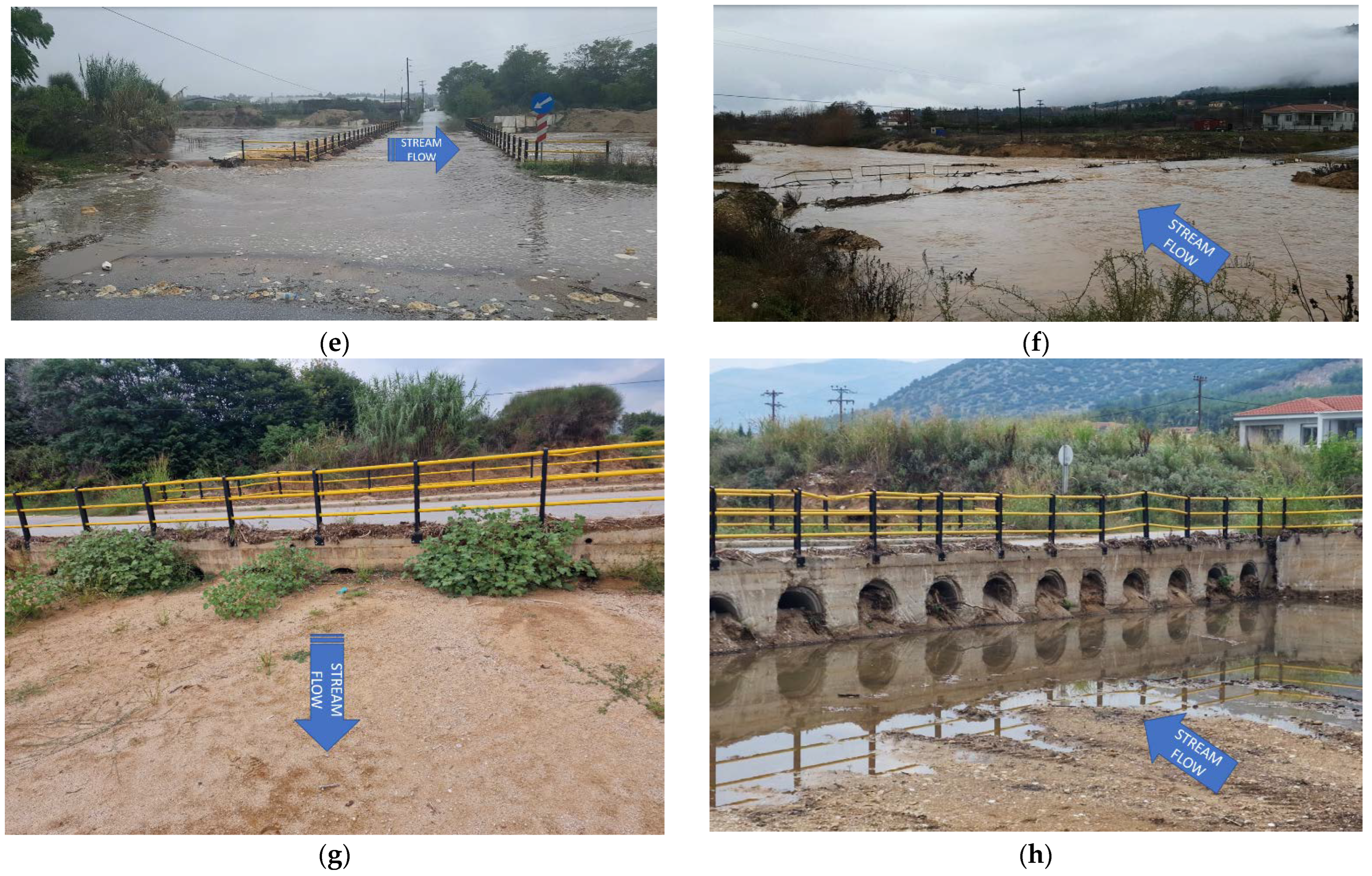
2.1. Case Study: Kallifitos Torrent, Greece

The case study is a reach of Kallifitos torrent at the suburbs of Drama City in Greece (Figure 1). The watershed area of the torrent is 115 km2. It is a typical intermittent Greek torrent that has flash flood risk potential after heavy rainfalls [56]. The flow can change in hours from no flow to a flow with great rapidity, carrying large amounts of water, sediments and debris [57]. Its headwaters start at Falakro Mountain, continuing its flow nearby the Kallifitos Village while it crosses through chutes under the city of Drama and finally discharges to Agia Barbara Stream, a tributary of Aggitis River [58]. The Aggitis River Basin is surrounded by different mountains. Specifically, to the west by the Menoikio Mountain, to the east by the Falakro Mountain to the southeast by the Ori Lekanis Mountain and to the southwest by the Paggeo Mountain [59]. The central section of Aggitis River Basin is cultivated for cereals such as wheat and barley and as you move further downstream with maize and cotton. The lowlands of the studied torrent are varied in bed width, channel slope, bank heights and slopes, with a meandering pattern and several anthropogenic interventions as it flows through the city of Drama. The location of the specific studied reach is at the east entrance of Drama City where there is also an Irish bridge (length: 45 m and width: 8 m) with 30 culverts of concrete pipes (diameter: 0.80 m and width: 8 m) [60,61]. The studied torrent reach is of high importance due to its proximity to Drama City, the fact that it causes frequent flooding and damages the road network and the Irish bridge and disrupts the city’s transportation. The torrent has a diversity of fluvio-geomorphologic changes in its channel and bed shape with large amounts of sediment transported, deposited and eroded during and after heavy rainfalls.

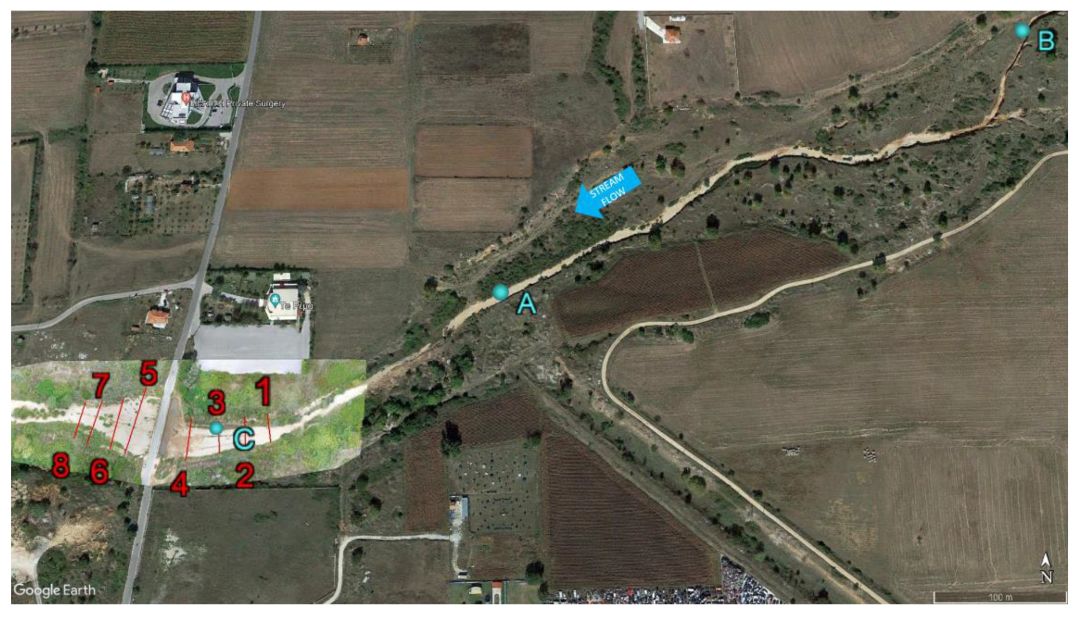
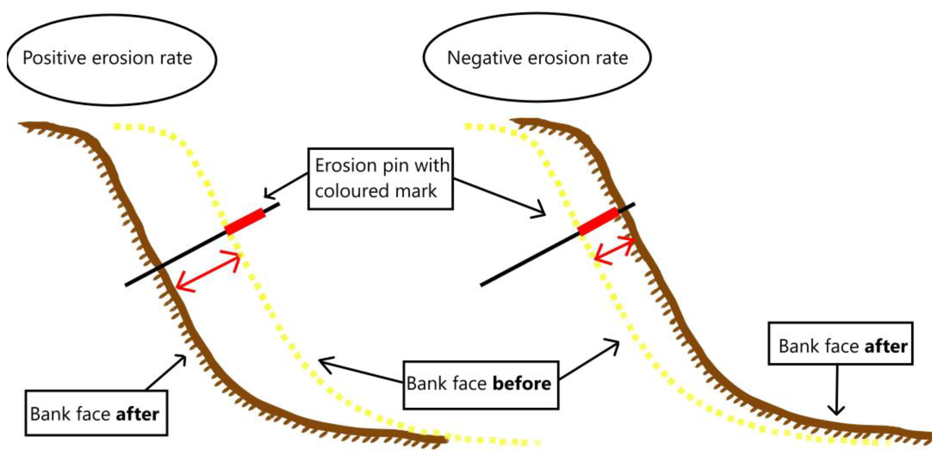
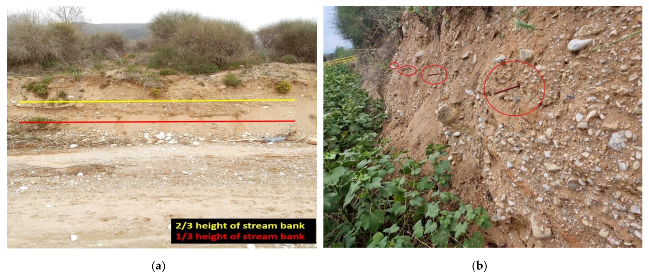
2.2. The Field Surveys: Cross-Sections and Erosion Pins

Two field methods were utilized: (a) cross-section survey (CS) [62] and (b) erosion pins [63]. Both methods were used to validate the results from the analysis of the UAV’s images. Eight cross-sections of the torrent were recorded in order to compare the dimension and any change among different events (Figure 2). Four of the CSs (1–4) were upstream from the Irish bridge and the other four (CS5–8) downstream to assess the potential impacts of the anthropogenic structure. The GPS/GNSS (Global Position System/Global Navigation Satellite System) RUIDE PULSAR R6P (Guangzhou, China) was selected to record the real coordinates (in WGS 84) of the eight cross-sections. Surveying channel cross-sections is a standard method to analyze and measure changes in stream channel geometry, such as stream bank and bed erosion and depositions [64].
The erosion pin method (Figure 3) was selected due to its practicability for short time-scale investigations and its results have high accuracy (up to 5 mm) [65]. The length of the pins was 80 cm, because erosion rates of up to 50 cm per erosion event were witnessed in similar-sized streams [66]. A pin diameter of 1 cm was selected because it was small enough to cause minimum disturbance to the banks but large enough to not bend under most high-discharge events [67]. A total of three erosion pins was installed. One of the plots was within the area captured by the drone flights while the others were upstream.
Each erosion pin plot included two horizontal rows of five pins each (Figure 4) installed on bare banks. Pins within these rows were placed 1 m apart for a total length of 4 m. To consistently place the pins in similar bank positions among the streambanks, the horizontal rows were placed at 1/3 and 2/3 of the height of the bank. The Kallifitos torrent has three erosion pin plots, specifically A: X:514557,150 Y:4554900,600, B: X:515011,382 Y: 4555136,200 and C: X:514334.900 Y:4554791.400 (see Table 1) in three different locations of the torrent (Figure 2). The specific reach (captured by the drone) includes only one pin, plot C. The measurement period is during the last winter (specifically the pins were installed in November 2021 and measured in March 2022 and June 2022).

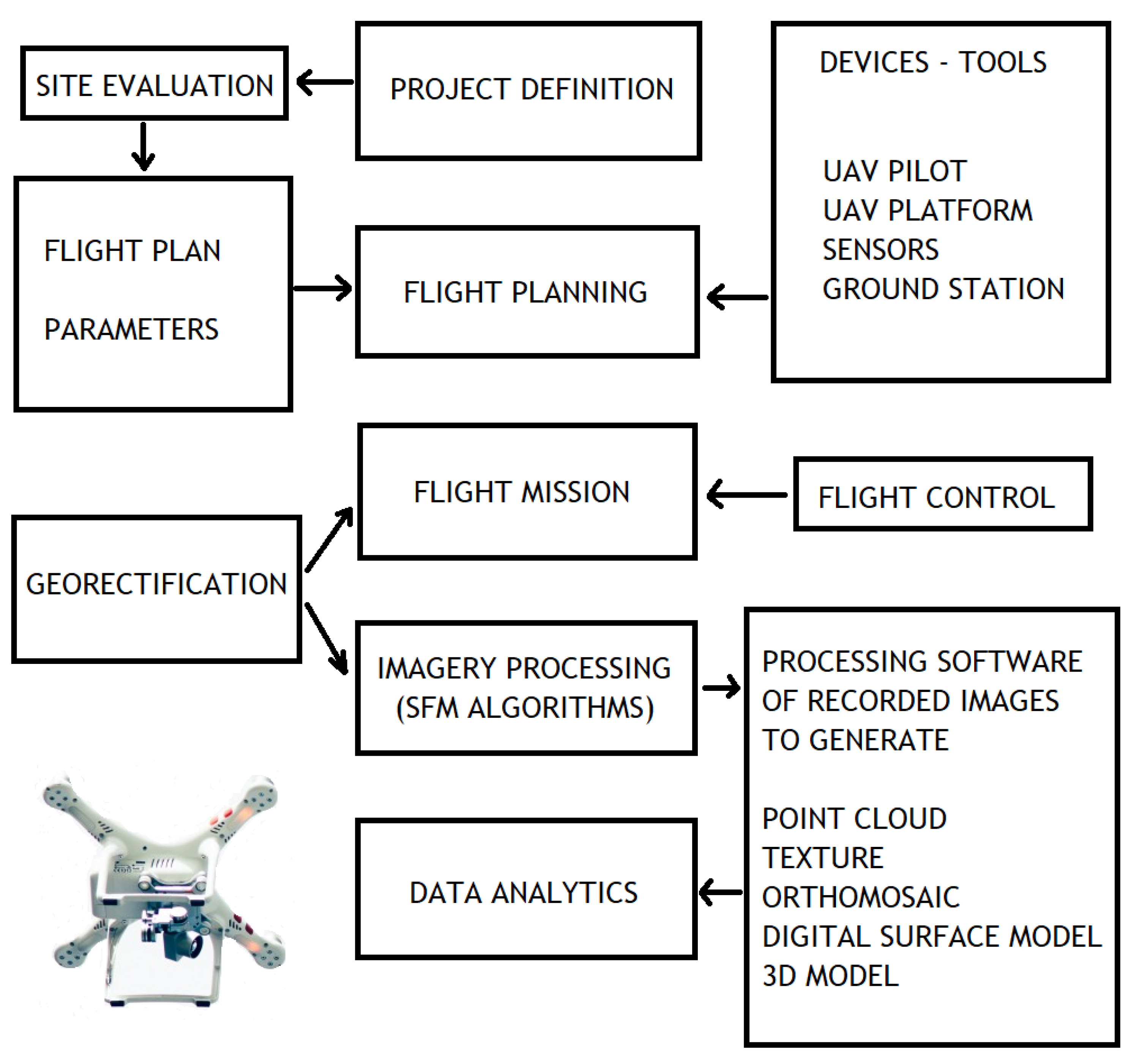
2.3. The Airborne Survey

A DJI Mavic 2 Pro was used to perform the airborne survey of the studied reach (Figure 2). Monitoring of Kallifitos torrent included flights through the year to capture the conditions before and after rainfall events or anthropogenic work (e.g., sand extraction by heavy-vehicle excavators). Specifically, six different flight missions were conducted to compare the outputs and monitor the fluvio-geomorphologic changes: (a) 24 September 2020 (Flight 1), (b) 5 January 2021 (Flight 2), (c) 11 January 2021 (Flight 3), (d) 18 March 2021 (Flight 4), (e) 18 June 2022 (Flight 5) and (f) 24 August 2022 (Flight 6). The particular drone that was used is a powerful quadcopter with a flight range of 31 min, weighting 734 gr and can be interfolded for easy transportation [68,69]. The RGB camera on the UAV is a 1′ CMOS (complementary metal oxide semiconductor) sensor with a resolution of 20 megapixels [70]. The drone-attached GPS system used is GPS/GLONASS (Geographic Position System/ Global Navigation Satellite System). The maximum operating range of the drone is 10 km, but this depends on the GPS signal, the weather conditions and the life of the battery. The Advanced Pilot Assistance System (APAS) technology helps to avoid obstacles in front or behind, while at the bottom it has an auxiliary light that keeps the sensors functional even in low-light conditions [71]. The UAV flights were conducted at 50 m height to capture detailed pictures of the torrent, commonly used for such monitoring [72]. The pictures were processed in the Pix4D software (Pix4D SA, Prilly, Switzerland) to produce the orthomosaics and digital surface models (DSMs) of the study reach. Pix4D is capable of combining and merging images based on common points, a characteristic methodology for photogrammetric applications [73]. Pix4D has a set of tools, including Pix4Dcapture as a mobile application to define and execute the flight plan and Pix4Dmapper that can be utilized to edit the captured data and create photogrammetric products [74]. The Pix4Dcapture is a mobile application that enables autonomous flight missions (grid, double grid, polygon, circular, free flight) and provides an estimated flight time that is calculated based on the defined mission parameters [75]. The Pix4Dmapper generates the point cloud, the mesh model, the texture, the orthomosaic, the 3D model (if images are captured from different angles) and the DSM. One of the Pix4D advantages, in comparison to other software, is the report feature and processing log which provide the processing results [76]. The software is widely known with vast photogrammetric applications and good documentation that also exports a report on the DSM and mosaic [77]. The UAV-based photogrammetry is able to produce highly accurate results due to Structure-from-Motion (SfM) and Scale-Invariant Feature Transformation (SIFT) algorithms [78]. The SfM algorithm is a user-friendly and low-cost alternative to traditional terrestrial techniques [79]. The SIFT algorithm and its variants provide invariant image transformation, rotation and scaling and good robustness to light changes, noise and affine transformation [80]. The photogrammetric process based on the UAV mission is depicted in Figure 5. The produced orthomosaics are visualized in Figure 6 while the DSMs based on the six different UAV flights are shown in Figure 7 (elevation height is above mean sea level). The Geomorphic Change Detection (GCD—available in ArcGIS toolbox) which is the Riverscapes Consortium’s longest running, best developed software with the largest user database worldwide [81] was used to compare elevation changes at the streambed. The GCD software was initially developed to detect topographic changes in rivers, but it can also work for simple change detection by comparing canopy records of any two surfaces [82]. Volumetric change (digital elevation model of differences—DoD) is calculated from the difference in the surface elevations from the digital surface models (DSMs) derived from the repeated topographic surveys [83]. In order to eliminate the vegetation interference, a mask was used to exclude the riparian vegetation as much as possible and to study the exact same area, as each DSM covered a different area in dimensions.

3. Results

3.1. Erosion Pin Plots Comparison

In pin plot “A” (Table 1), during the first period of measurements (February–March 2022), the results showcased that the bottom part of the stream bank (1/3) in four points had limited erosion, ranging from 1 to 7 cm. One of the pins had a negative reading, meaning material deposition that reached 7cm. On the upper part of the streambank (2/3), the maximum erosion was 10 cm. In pin plot “B” (Table 1), on the bottom part, four of the five pins recorded erosion greater than 40 cm. On the upper part, three of the five pins also had erosion greater than 50 cm. In pin plot “C” (Table 1), on both the bottom-part and the upper-part pins, the erosion was substantially higher (greater than 50 cm) than the other two erosion pin plots. The three erosion pin plots showcased the high spatial variability in streambank erosion, even within one plot and among plots.
In the second period of measurements (June 2022), small changes were recorded because of the low stream flows and absence of rainfall events. In pin plot “A” (Table 1), on the bottom part of the stream bank (1/3) in four of the five, no erosion was recorded. On the upper part of the stream bank (2/3), the erosion was very limited, ranging from 1 to 2 cm. In pin plot “B” (Table 1), on the bottom part and on the upper part, erosion was not recorded at any of the pins. In pin plot “C” (Table 1), on the bottom part, four of the five pins had deposition that ranged from 2 to 23 cm. On the upper part, the maximum erosion was recorded as 6 cm.

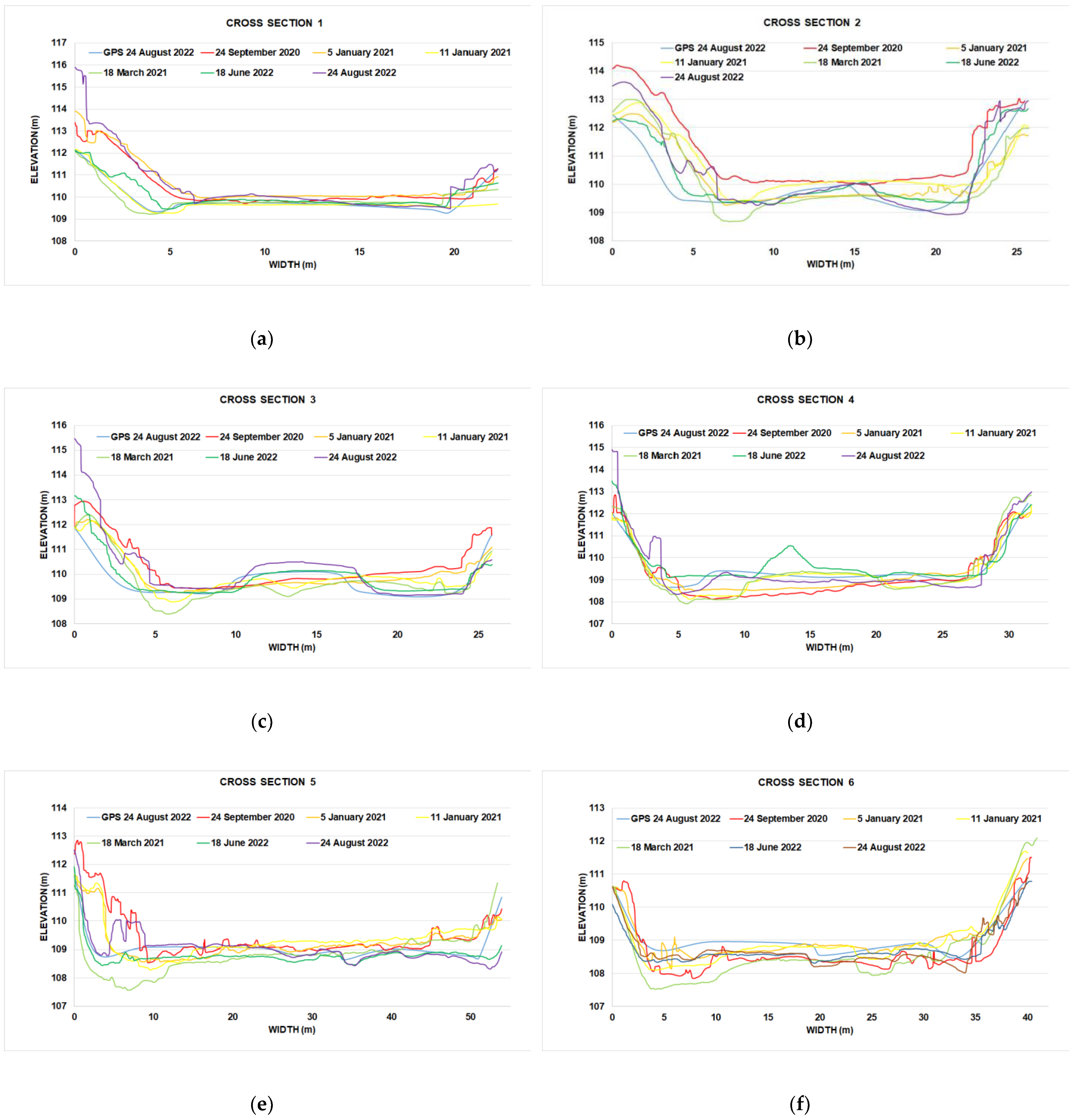
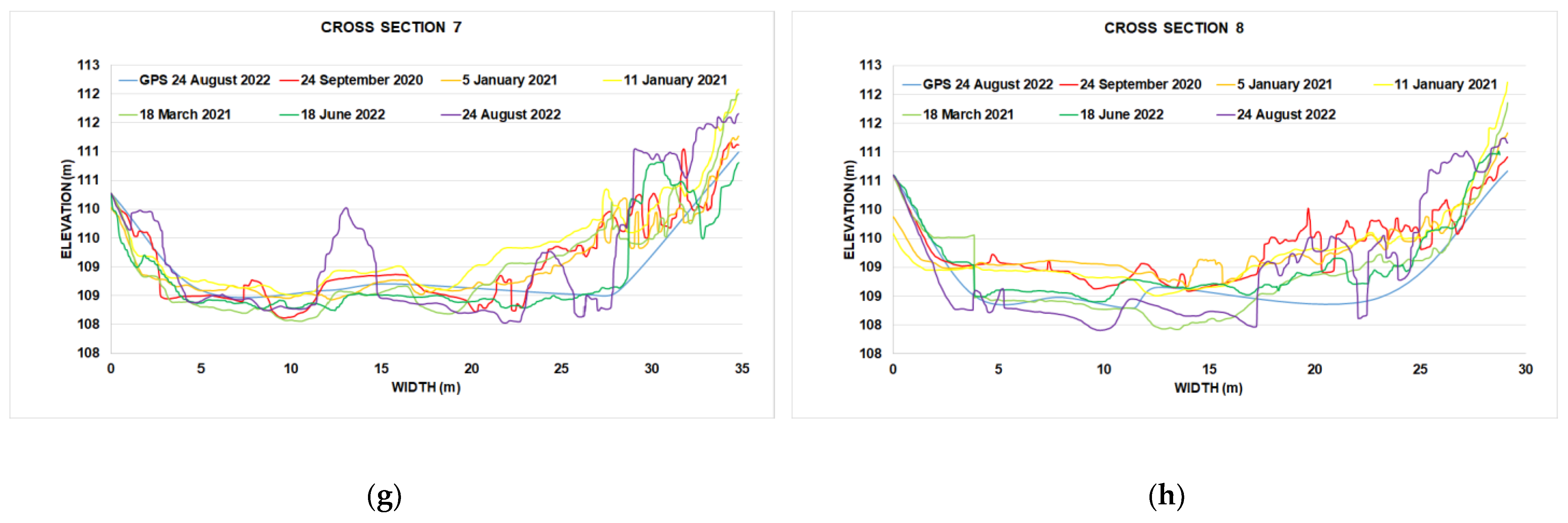
3.2. Cross-Section Comparison
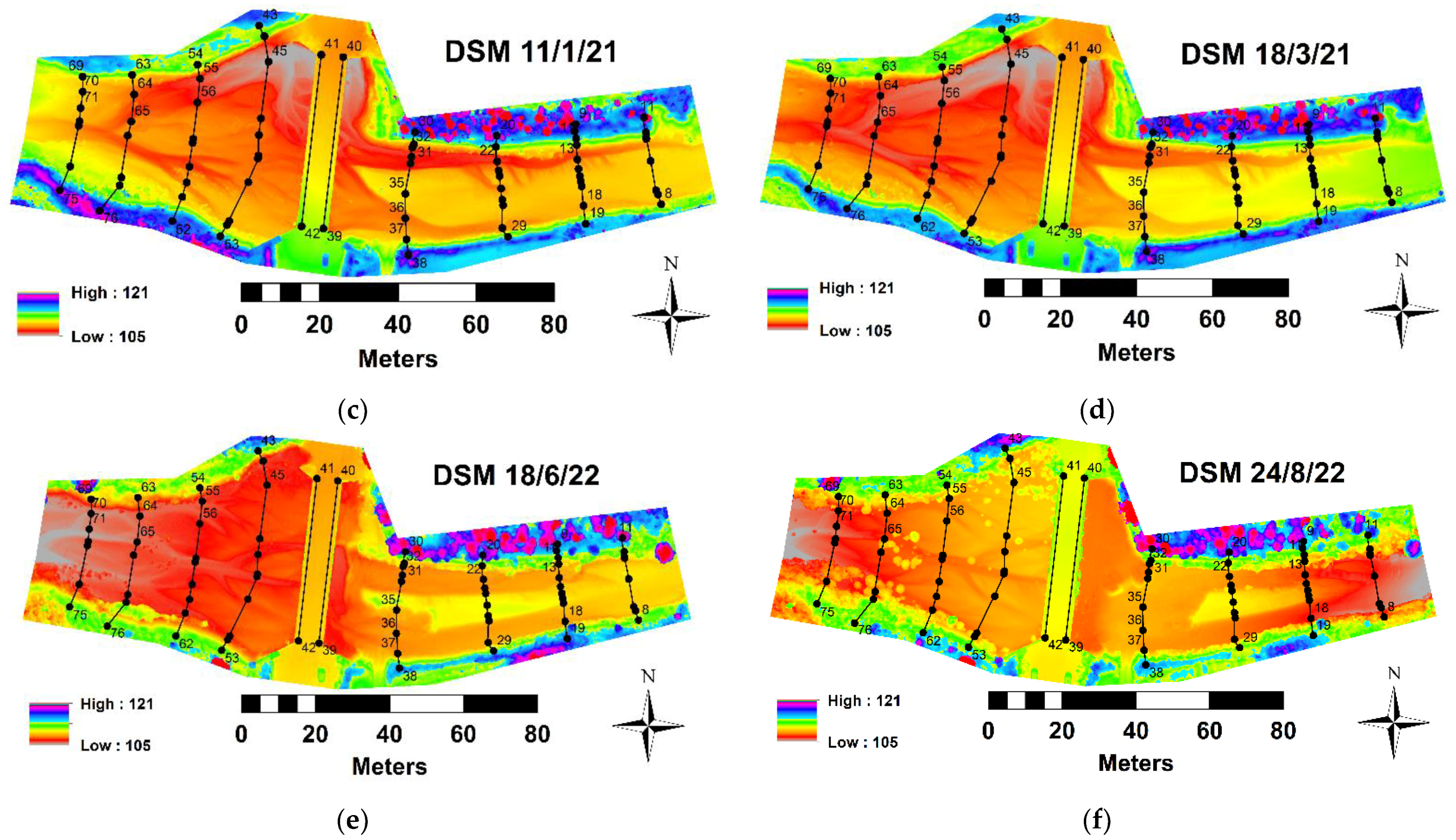
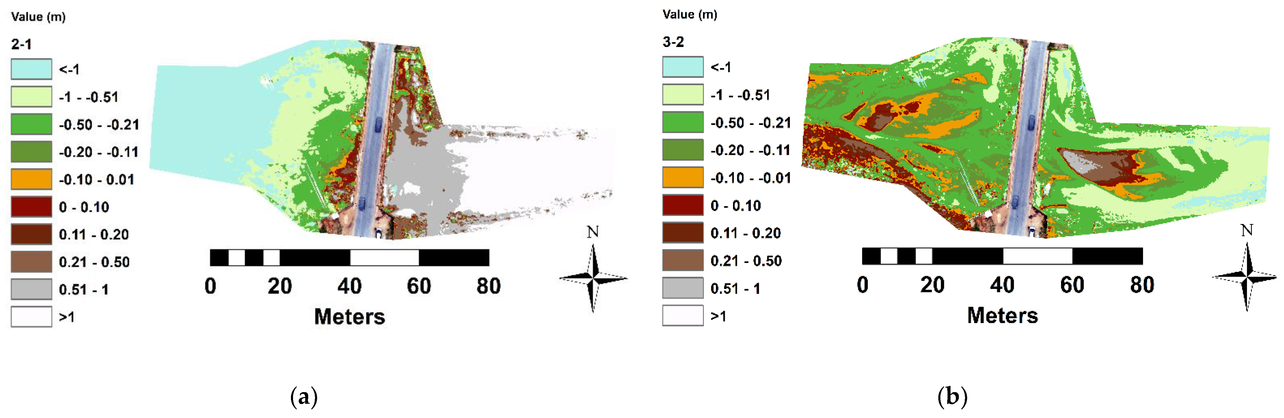
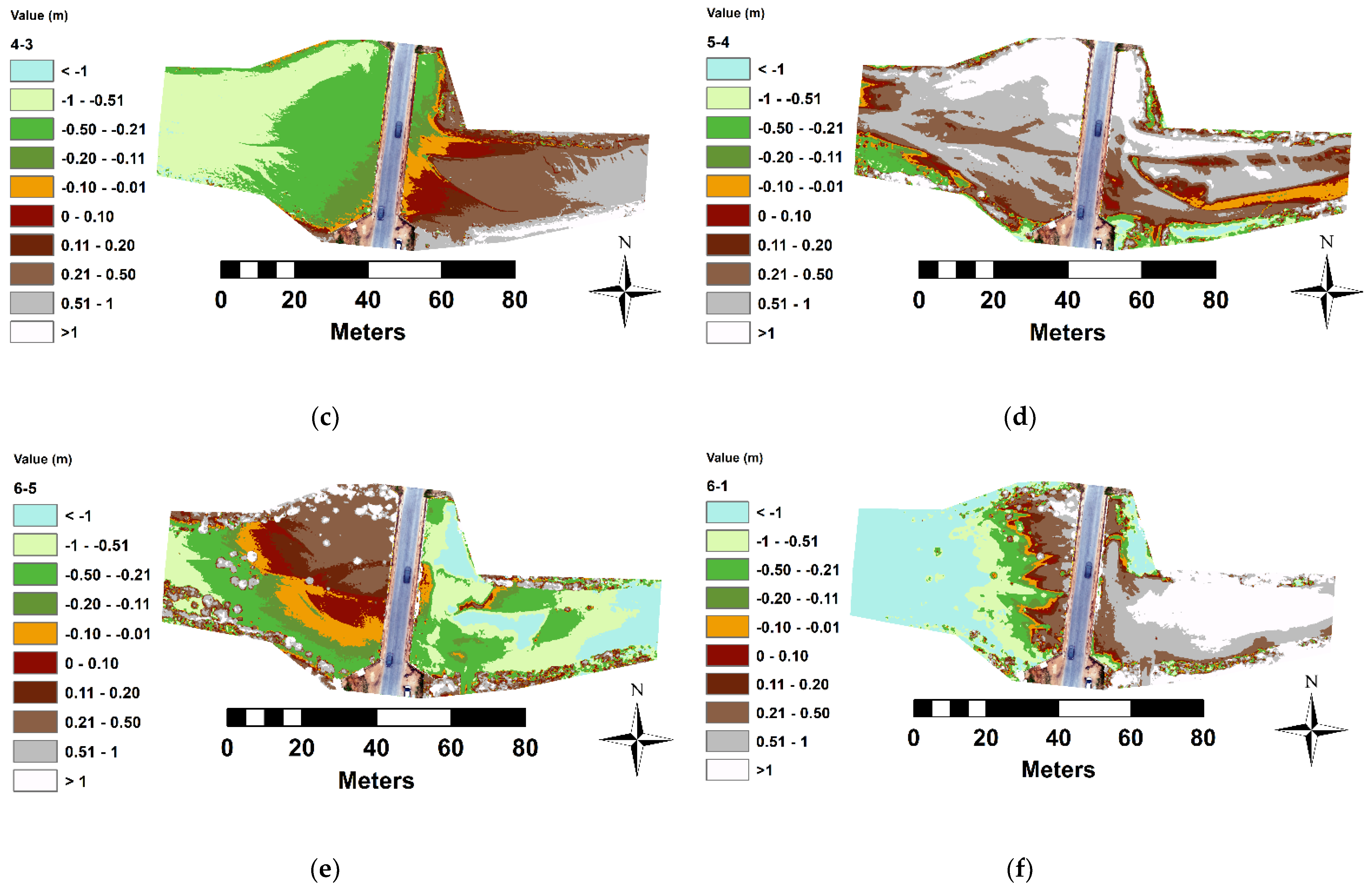
The eight cross-sections (see Figure 2), produced based on the field measurement (using the GPS), were compared with those produced from the drone images flown in the six different periods along the study’s stream reach. In this comparison, the left bank is the north bank and the right bank is the on south (see Figure 2). Firstly, the GPS cross-section was compared to the cross-section produced by Flight 6 that took place on the same day as the GPS measurements. The GPS lines are blue and the drone lines are purple (Figure 8). Comparison of all eight cross-sections showed an almost identical match along the stream bed but there were small deviations on the left and right banks as a result of the presence of the riparian vegetation (Figure 8).
Figure 8 also includes the drone cross-section produced from the five other flights: (a) Flight 1 (red line), (b) Flight 2 (orange line), (c) Flight 3 (yellow line), (d) Flight 4 (light green line) and (e) Flight 5 (green line). Following is a comparison of all six flights together. When comparing the cross-sections, starting from CS1, we can identify the almost identical match on the stream bed and on the right bank. However, on the left bank, we can see slight deviation in the slopes. That should be expected since there is a lot of tall and dense vegetation that induces those errors on the DSM products (Figure 8a). For CS2, there was a small deviation again on the left slope because of the vegetation’s presence. In the stream bed, there is a small fluctuation in the elevation’s values between the different flights. This is a result of depositional events at this cross-section (Flights 3–5). These deposits were collected by the municipality’s excavators (Flight 1) (Figure 8b,c). There is a match at approximately 90% of the different flights at the CS3 (Figure 8c). An increase is observed in the bed elevation between the bed width distance 10 to 17 m (Flights 5,6) due to deposition and the water moving around the island developed in the middle of the stream bed due to the excessive deposition. At CS4 (Figure 8d), the GPS and the three flights (Flights 3,5,6) have the same elevation. Flights 2 and 4 (red and yellow line) are 70 cm lower than the previous cross-section due to the municipality’s excavator works, which removed the deposited material. This removal is a significant disturbance to the riverine ecosystem but is a necessity because, otherwise, even small-scale floods can overflow the Irish bridge and cause traffic jam problems. At CS5 and CS6 (Figure 8e and Figure 8f, respectively), the elevation and slopes are the same at approximately 95% of the produced cross-sections. In cross-section CS7 (Figure 8g), in the middle section of the stream bed, the elevation of the drone images increases approximately by 1 m and that is because of the riparian vegetation found in the area. This vegetation appeared taller and denser during the growing season. The right bank also shows steeper slopes due to the vegetation. Finally, for the last cross-section, CS8 (Figure 8h), a few small changes were detected only on the right bank, again because of the density and height of the vegetation.
In the following paragraphs, comparisons of successive pairs of flights for each cross-section are described. In these comparisons, when the slope profile distance from the stream centerline increased, we considered erosion occurring (from this point on, mentioned as “increased”). In contrast, when the slope profile distance decreased from the stream centerline (from this point on, mentioned as “decreased”), we considered deposition occurring. In regard to the stream bed, when it is elevated, it indicates deposition, while when it is lowered, it indicates degradation (erosion).
Specifically, when comparing Flight 1 and 2 at CS1, there were no change on the bed and the banks. At CS2 and CS3, there was an increase on the stream bed elevation while the distance of both banks decreased, indicating material deposition. The slopes at both banks were the same at CS4, while the stream bed was elevated. In CS5, both bank slopes increased their distance while the bed elevation was lower, probably because of the erosion. At CS6, the slope profile was the same. The elevation on the stream bed was higher and, at the right bank, the slope distance decreased, probably due to deposition. At CS7, we have no change on the slopes of both banks but we noticed both deposition and erosion along the stream bed at different locations (elevation both increased and decreased). Finally, in CS8, erosion was most likely recorded since the slope distance increased and the elevation of the stream bed decreased.
At CS1, when comparing Flights 2 and 3, it is most likely that we had deposition since the stream bed was elevated and the bank distances were decreased. CS2 had a different pattern, with the slope profile distance increasing on the left bank (probably due to erosion), while the stream bed was elevated (probably due to deposition) and on the right bank, the slope profiles were similar. The left bank of CS3 had similar slope profiles, while the stream bed probably had deposition (was elevated) and the right bank had erosion since its distance increased. Both bank slope profiles at CS4 increased their distance from the stream centerline (erosion events) while the stream bed was elevated (deposition events). At CS5 and CS6, the bed elevation and bank slope profiles remained the same. The slope distance decreased from the stream centerline on the right bank and the stream bed was elevated (due to deposited material). Finally, at CS8, the stream bed (elevated) and left bank (increased distance) probably experienced erosion, while the right bank had deposition (slope profile distance decreased).
For Flights 3 and 4, at CS1, the left bank distance was increased while the stream bed was elevated and the right bank decreased. Both banks remained the same at CS2, while the stream bed seemed to be degraded (lowered elevation). At CS3 and CS4, only the left bank changed, although for part of the slope profile, the distance increased (eroded), while for another part of the profile, the distance decreased (aggraded). In the stream bed, we observed an elevation decrease, probably because of erosion. The stream bed seems to be elevated while for the right bank slope profile, the distance decreased, probably due to the deposition. CS5 was the most consistent, with banks and beds probably experiencing erosion (bed with lower elevation and both banks with increased distances). At CS6 and CS7, only the stream bed lowered (erosion). Finally, at CS8, both phenomena were identified as the left bank slope profile distance decreased (deposition) while the right bank distance increased (erosion) and at the stream bed, a lower elevation was recorded (degradation).
Moving on to the comparison between Flights 4 and 5, only the left bank changed at CS1, with slope profile distance decreasing, indicating deposition. In contrast, at CS2 and CS3, the left banks, the slope profile distance increased, indicating erosion. This was verified, as the erosion pins in plot C that were installed in exactly the same location as CS3 on the left bank and measured a similar period with flights 4 and 5. The results of the pins in plot C can be seen in Table 1, with most pins recording erosion greater than 50 cm, validating the results of the left bank at CS3. At CS4, both banks increased their distance (erosion) while the stream bed was elevated (deposition). The stream bed at CS5 was also elevated while the banks had opposite trends; the left bank slope profile distance increased and the right one decreased its distance. Deposition only on the stream bed was also present at CS6, CS7 and CS8, since they were elevated. Finally, at CS8, the left bank changed with slope profile, decreasing its distance (deposition).
During the period between Flights 5 and 6, only the left bank changed at CS1 and CS2, with the slope profile distance decreasing (deposition). At CS3, the left bank also changed with the slope distance increasing (probably eroded), while the bed elevation increased (deposition). The stream bed elevation at CS4 decreased (erosion), while the right bank decreased distance (deposition). In contrast, downstream at CS5, we noticed deposition at the bed (elevated), while the two banks had opposite trends, with the left bank experiencing deposition (decreased distance) and the right one erosion (increased distance). Both stream beds at CS6 and CS7 were elevated. In addition, in CS7, for both bank slope profiles, the distance decreased. Finally, at CS8, the stream bed appeared degraded (decreased elevation) and the right bank increased distance but the left one remained the same.

3.3. DSM Comparison

The GCD tool enabled us to compare the different DSMs created by the drone flights (Figure 9). More specifically a ten-level scale ranging from <−1 to >1 was developed. For the positive value scale, the categories were: (a) >0–0.10 low deposition, (b) 0.11–0.20 moderate deposition, (c) 0.21–0.50 high deposition, (d) 0.51–1 very high deposition and (e) >1 severe deposition. For the negative values, the categories were (f) 0–(−0.10) low erosion, (g) (−0.11)–(−0.20) moderate erosion (h) (−0.21)–(−0.50) high erosion, (i) (−0.51)–(−1) very high erosion and <−1 severe erosion. In Figure 9a, when comparing the DoD from Flights 1 and 2, it is evident that upstream from the bridge, we have a deposition ranging from 50 cm to 1 m in the center of the stream bed. For the period between Flights 2 and 3, upstream had erosion on the left and right bank, ranging from 20 to 50 cm, and deposition at some points along the stream bed, ranging from 20 to 100 cm (Figure 9b). Increased deposition at the upstream section of the torrent from the bridge with moderate erosion downstream was also found when comparing the DoDs of Flights 3 and 4 (Figure 9c). Severe deposition upstream and downstream on the stream bed was found for the DoD based on Flights 4 and 5, especially near to the north bank of the torrent. The results of the DoD also match the results from the pins that were installed upstream (see Figure 2). Specifically, erosion pin plot C recorded erosion greater than 50 cm (see Table 1) and in Figure 9d, on the north bank, where the pins are placed, the erosion captured is 0.51–1.00 (gray color) or greater than 1.00 m (white color). In Figure 9e (Flights 5 and 6), the upstream reach has high erosion while the downstream has high deposition, especially near to the north bank. Comparing Flight 6 (the last) with Flight 1 (the first) (see Figure 9f) showcases severe deposition on the upstream and some deposition immediately downstream from the bridge but further downstream, it has erosion. Finally, when comparing the DoD from Flight 6 with the DoDs from other Flights (2–4), the same trend is present with high deposition upstream, especially near to the north slope and moderate erosion in the middle section of the stream bed. Downstream, there is severe deposition in the middle section of the stream bed and to the north bank and high deposition from the south bank to the middle section of the stream bed. The results from the DoDs seem to be highly validated in comparison to the field measurements (erosion pins and cross-sections) during the examined periods. The torrential character of Kallifitos reach is depicted in Figure 10, with different events of sand extraction (Figure 10a,b,h) deposition (sediment and other material) (Figure 10c,d,g) and flooding (Figure 10e,f). The extraction from the streambed was performed using heavy vehicles (trucks and excavators) to remove the debris, which fills the culverts of concrete pipes under the bridge (Figure 10g,h).

4. Discussion

When comparing the eight CSs and the DoDs from flight to flight, many changes were recorded along the stream banks and bed. In addition, in the comparisons among the flights, different trends were recoded, even in the same periods from CS to CS, for example, some having erosion and others deposition. Differences were also recorded for the same CS (C.S.2 Figure 7b), even in the same period, for example, erosion on one bank, deposition on the other and deposition on the bed. These trends were expected since fluvio-geomorphological events, such as bank erosion and deposition and bed degradation, are typically sudden and episodic events that lead to their high temporal variation [84,85,86].
For long periods (decades) of monitoring erosion, series of topographic maps or aerial and satellite images are utilized [87,88,89]. For shorter time scales, actual field studies are conducted utilizing either erosion pins [90,91,92] or CSs [93]. These methods allow one to estimate stream channel and deposition more accurately (higher resolution) compared to the long-time-scale methods. The short-term methods are unfortunately time consuming and are spatially and temporally very limited. The utilization of new technologies (UAVs) can allow for the shortcomings of the long- and short-term scale methods.
Worldwide, significant yearly and seasonal variations have been recorded in stream erosion and deposition [94]. Zaimes et al. found significant differences in seasons that indicate the need for frequent (at least seasonal) measurements, since yearly measurements can mask some of the processes that are occurring (particularly deposition events) [95]. To resolve the temporal issue in the past, several tools have been developed, such as photo-electronic erosion pins (PEEPs) [96], the thermal consonance timing (TCT) [97] and the Automated Soil Erosion Monitoring System (ASEMS) [98]. All three of these can have very high temporal resolution but are again limited spatially, as most field methods are. Through the use of UAVs, the spatial scale is significantly increased, since it can cover an entire reach, including both banks and the stream bed. Another advantage is because the flight covers a larger area, the flight requires significantly less time than field measurements’ and can be conducted more. Finally, the use of UAVs is safer since the researcher does not enter the stream channel [99].
It has been recorded in many different regions of the world that watershed area, shape and slope, watershed and riparian vegetation cover and land use, topography, geology, soil bank and bed composition and strength, antecedent soil moisture, stream morphology, pattern and order, channel characteristics and stage, climate and weather cycles, hydrologic regime, floods and droughts and disturbance history [100,101] are factors that substantially influence stream bank and bed erosion and deposition processes [102]. The fact that so many factors influence erosion and deposition is why a more holistic view of the channel is required to be able to fully understand the complex process taking place. The produced UAV CS covers both stream banks and the bed but covering a significantly larger area than the erosion pins. In addition, the UAV drones capture and record substantially more measuring points than the GPS CS, in significantly less time. Of course, the main concern is to produce UAV CSs that meet the measuring accuracy of erosion (cm) of the GPS cross-sections. The results of this study are encouraging, although we believe that better calibration is a necessity to reach the GPS and other field measurement accuracy. The images in this study were obtained parallel to the surface plane. The accuracy of these methods can be increased if images are captured at different angles [103]. Oblique images, obtained at an angle < 15 degrees, can reduce the image’s deformation and the systematic topographic error [104]. Of course, this shortcoming of the UAV images can be compensated because of the other cross-sections that can be developed from them. Even more advantageous is the development of the orthomosaic that covers the entire reach and can assess if the dynamic equilibrium is maintained (deposited material equal to eroded material). Specifically, we can calculate, for the entire reach, how much deposition and erosion we had for a specific period and actually see if the reach had erosion, deposition or it maintained its dynamic equilibrium (deposition equal to erosion).
Streams are in a state of dynamic equilibrium and changes or disturbances at the watershed or reach level, upstream and downstream, lead to the stream responding via different process (e.g., erosion or deposition of the bank or bed) to reach a new equilibrium state. The dynamic equilibrium of streams is dependent on discharge, slope, sediment load and sediment size [105]. In this study, the large deposition of material (Flights 3–6 and CS 2–4), especially upstream from the bridge, indicates significant disturbances are occurring. Actually, in order to be able to maintain the channel shape, human intervention is conducted. Specifically, almost every year, the municipality excavators come and remove the excess sediment deposited. It is essential to try to implement a watershed approach and try to distinguish what are the disturbances that the area is experiencing that is leading to this excessive sediment supply and deposition. The use of UAV images that capture larger areas more frequently and more cost effectively can enhance the ability to identify the disturbances compared to the traditional methods. This will allow land and water managers to find more sustainable solutions for the study reach compared to the current one (removing the sediment with excavators). Nature-based solutions should be adopted that provide long-term solutions. An example of a successful, simple and inexpensive method to mitigate erosion is the re-establishment of perennial vegetation along eroding stream banks and riparian areas [106].
The presence and the condition of the riparian vegetation on stream banks is a key factor for fluvio-geomorphologic processes, including stream bank erosion and deposition [107]. Perennial plant communities with vigorous root systems, regardless of whether they are trees or grasses, increase stream bank stability, especially in headwater streams [108]. In this study, this was evident in CS2 and CS3 (Flights 1 and 6).
Spatial differences along the stream bank profile have also been recorded in many cases. Different studies have found contradicting results regarding erosion in the top and bottom banks [109]. The traditional methods (pins and CSs) can have a limited number of points along the profile compared to UAV images. Using a laser scanner appears to be the optimal solution because of the high resolution of the captured images [110]. Based on the results of the study, UAV images can also provide the entire bank profile and channel CS but are more flexible since they will require less set-up time compared to the laser scanner. For example, in this study, the advantage of UAVs can be seen at CS3 and CS4. When comparing Flights 3 and 4, erosion was detected on the top part and deposition at the lower part.
Human infrastructure, at both the reach and watershed scale, can also alter erosion and deposition process and rates (see Figure 2) [111]. In this case, we focused on the Irish bridge (See Figure 2). Specifically, four of the cross-sections were upstream from the bridge while the other four were downstream (Figure 6). The upstream cross-sections (1–4) and channel had typically more deposition than the downstream cross-sections and areas (see Figure 8 and Figure 9). This clearly showcases how human intervention can alter the dynamic equilibrium of stream ecosystems. At this point, we must notice that the Irish bridge, by accident, might be acting as a protective mechanism since, because of this barrier, the sediment is deposited and does not move further down, causing potential damage to the city of Drama. Of course, this is just a short-term solution and a more holistic and watershed solution is required. The use of UAVs to monitor such problems with infrastructure can help protect them more cost effectively and provide more sustainable solutions.

5. Conclusions

Overall, the significant yearly and seasonal channel changes indicate the need for long-term datasets. In addition, the high spatial variations, even within a reach of less than 1 km, indicate that frequent spatial measurements are needed to fully understand the fluvio-geomorphological processes occurring. This complex information is required for managers to be able to understand and predict stream bank and bed erosion and deposition accurately, thus, to provide sustainable cost-effective mitigation management plans and practices [112]. This methodology can provide this information by providing data with high spatial temporal accuracy and at relatively large scales.
The Water Framework Directive (WFD) (2000/60/EC) and the Flood Directive (FD) (2007/60/EC) are the fundamental European tools on sustainable water management. To be able to implement these two directives, fluvio-geomorphological research and monitoring in riverine environments are key components that can be provided by the methodology described in this study [113]. Developing, identifying and adopting cost-effective methods for stream channel erosion and deposition are essential for understanding the processes degrading riverine ecosystems and increasing flooding risk potential [114].
The methodology of this study also helps resolve several issues, highlighted in previous studies in regard to spatial and temporal scales [115,116,117]. The use of images captured by UAVs led to a cost-effective methodology. The spatial and temporal information provided by these images help explain the timeline of erosional and depositional events in stream beds and banks. The cross-sections based on the UAV were validated with field measurements (GPS and cross-sections), with overall good results. Still, the quality of the results can be impeded by: (a) weather conditions, (b) presence of dense and tall vegetation in the riparian area, stream banks and bed, (c) flight parameters, e.g., height, (d) shadows and associated terrain-shading errors and (e) GCPs and georeferencing processes [118,119,120,121,122,123]. The results of this study showcase progress in enhancing the spatial and temporal accuracy of stream channel (bank and bed) monitoring. Still, despite its shortcoming, we strongly recommend the adoption of this method by the responsible management authorities to assess fluvio-geomorphological changes, particularly in stream reaches near or in cities.

Author Contributions

Conceptualization, G.N.Z. and P.D.K.; methodology, G.N.Z. and P.D.K.; validation, I.K.K.; formal analysis, G.N.Z., G.T.G. and P.D.K.; investigation, G.T.G.; data curation, G.T.G., I.K.K. and P.D.K.; writing—original draft preparation, P.D.K.; writing—review and editing, G.N.Z., P.D.K., G.T.G. and V.I.; visualization, G.T.G., P.D.K. and I.K.K.; supervision, G.N.Z. and V.I.; project administration, G.N.Z. All authors have read and agreed to the published version of the manuscript.

Funding

This research was funded in frames of the Joint Operational Black Sea Programme 2014–2020 and the Project BSB 963 “Protect-Streams-4-Sea”, with the financial assistance of the European Union through the European Neighborhood Instrument and by the participating countries: Armenia, Bulgaria, Georgia, Greece, Republic of Moldova, Romania, Turkey and Ukraine. Its contents are the sole responsibility of the authors and do not necessarily reflect the views of the European Union.

Data Availability Statement

Not applicable.

Acknowledgments

To Georgios Pagonis who helped during the field measurements with erosion pins.

Conflicts of Interest

The authors declare no conflict of interest. The funders had no role in the design of the study; in the collection, analyses, or interpretation of data; in the writing of the manuscript; or in the decision to publish the results.

References

  1. Costigan, K.H.; Kennard, M.J.; Leigh, C.; Sauquet, E.; Datry, T.; Boulton, A.J. Flow regimes in intermittent rivers and ephemeral streams. In Intermittent Rivers and Ephemeral Streams; Datry, T., Bonada, N., Boulton, A., Eds.; Academic Press: Cambridge, MA, USA, 2017; pp. 51–78. [Google Scholar]
  2. Tzoraki, O.; Nikolaidis, P.N. A generalized framework for modeling the hydrologic and biochemical response of a Mediterranean temporary river basin. J. Hydrol. 2007, 346, 112–121. [Google Scholar] [CrossRef]
  3. Dotterweich, M. The history of soil erosion and fluvial deposits in small catchments of central Europe: Deciphering the long-278 term interaction between humans and the environment—A review. Geomorphology 2008, 101, 192–208. [Google Scholar] [CrossRef]
  4. Tzoraki, O.; Nikolaidis, N.; Skoulikidis, N. Evaluation of in-stream processes of four temporary rivers. Geophys. Res. Abstr. 2005, 7, 02256. [Google Scholar]
  5. Zaimes, G.; Iakovoglou, V.; Emmanouloudis, D.; Gounaridis, D. Riparian areas of Greece: Their Definition and Characteristics. J. Eng. Sci. Technol. Rev. 2010, 3, 176–183. [Google Scholar] [CrossRef]
  6. Burchsted, D.; Daniels, M.; Thorson, R.; Vokoun, J. The river discontinuum: Applying beaver modifications to baseline conditions for restoration of forested headwaters. BioScience 2010, 60, 908–922. [Google Scholar] [CrossRef] [Green Version]
  7. Zaimes, G.N. Mediterranean Riparian Areas- Climate change implications and recommendations. J. Environ. Biol. 2020, 41, 957–965. [Google Scholar] [CrossRef]
  8. Llasat, M.C.; Llasat-Botija, M.; Prat, M.A.; Porcu, F.; Price, C.; Mugnai, A.; Lagouvardos, K.; Kotroni, V.; Katsanos, D.; Michaelides, S.; et al. High-impact floods and flash floods in Mediterranean countries: The FLASH preliminary database. Adv. Geosci. 2010, 23, 47–55. [Google Scholar] [CrossRef] [Green Version]
  9. Gaume, E.; Bain, V.; Bernardara, P.; Newinger, O.; Barbuc, M.; Bateman, A.; Blaškovičová, L.; Blöschl, G.; Borga, M.; Dumitrescu, A.; et al. A compilation of data on European flash floods. J. Hydrol. 2009, 367, 70–78. [Google Scholar] [CrossRef] [Green Version]
  10. Wilford, D.J.; Sakals, M.E.; Innes, J.L.; Sidle, R.C.; Bergerud, W.A. Recognition of debris flow, debris flood and flood hazard through watershed morphometrics. Landslides 2004, 1, 61–66. [Google Scholar] [CrossRef] [Green Version]
  11. Lowrance, R.; Leonard, R.; Sheridan, J. Managing riparian ecosystems to control nonpoint pollution. J. Soil Water Conserv. 1985, 40, 87–91. [Google Scholar]
  12. Yujun, Y.I.; Zhaoyin, W.; Zhang, K.; Guoan, Y.U.; Xuehua, D. Sediment pollution and its effect on fish through food chain in the Yangtze River. Int. J. Sediment Res. 2008, 23, 338–347. [Google Scholar]
  13. Wohl, E. Legacy effects on sediments in river corridors. Earth-Sci. Rev. 2015, 147, 30–53. [Google Scholar] [CrossRef]
  14. Bat, L.; Özkan, E.Y. Heavy metal levels in sediment of the Turkish Black Sea coast. In Oceanography and Coastal Informatics: Breakthroughs in Research and Practice, 2nd ed.; Khosrow-Pour, M., Ed.; IGI Global: Hershey, PA, USA, 2019; pp. 86–107. [Google Scholar]
  15. Liu, A.; Duodu, G.O.; Goonetilleke, A.; Ayoko, G.A. Influence of land use configurations on river sediment pollution. Environ. Pollut. 2017, 229, 639–646. [Google Scholar] [CrossRef]
  16. Zaimes, G.N.; Iakovoglou, V.; Syropoulos, D.; Kaltsas, D.; Avtzis, D. Assessment of Two Adjacent Mountainous Riparian Areas along Nestos River Tributaries of Greece. Forests 2021, 12, 1284. [Google Scholar] [CrossRef]
  17. Koutalakis, P.; Zaimes, G.N.; Iakovoglou, V.; Ioannou, K. Reviewing soil erosion in Greece. Int. J. Geol. Environ. Eng. 2015, 9, 936–941. [Google Scholar]
  18. Wischmeier, W.H. Estimating the soil loss equation’s cover and management factor for undisturbed areas, in Present and prospective technology for predicting sediment yields and sources. Agric. Res. Serv. Pub. 1975, ARS-S-40, 118–124. [Google Scholar]
  19. Zaimes, G.N.; Kasapidis, I.; Gkiatas, G.; Pagonis, G.; Savvopoulou, A.; Iakovoglou, V. Targeted placement of soil erosion prevention works after wildfires. In Proceedings of the IOP Conference Series: Earth and Environmental Science, Online, 26–28 August 2020. [Google Scholar]
  20. Dragičević, N.; Karleuša, B.; Ožanić, N. Erosion potential method (Gavrilović Method) sensitivity analysis. Soil Water Res. 2017, 12, 51–59. [Google Scholar] [CrossRef] [Green Version]
  21. Kostadinov, S.; Dragićević, S.; Stefanović, T.; Novković, I.; Petrović, A.M. Torrential Flood Prevention in the Kolubara River Basin. J. Mt. Sci. 2017, 14, 2230–2245. [Google Scholar] [CrossRef]
  22. Gholami, V.; Sahour, H.; Amri, M.A.H. Soil erosion modeling using erosion pins and artificial neural networks. Catena 2021, 196, 104902. [Google Scholar] [CrossRef]
  23. Tufekcioglu, M. Gully and streambank erosion and the effectiveness of control measures in a semi-arid watershed. Fresenius Environ. Bull. 2018, 27, 8233–8243. [Google Scholar]
  24. Arthun, D.; Zaimes, G.N. Channel changes following human activity exclusion in the riparian areas of Bonita Creek, Arizona, USA. Landsc. Ecol. Eng. 2020, 16, 263–271. [Google Scholar] [CrossRef]
  25. Anache, J.A.; Wendland, E.C.; Oliveira, P.T.; Flanagan, D.C.; Nearing, M.A. Runoff and soil erosion plot-scale studies under natural rainfall: A meta-analysis of the Brazilian experience. Catena 2017, 152, 29–39. [Google Scholar] [CrossRef]
  26. Zaimes, G.N.; Ioannou, K.; Iakovoglou, V.; Kosmadakis, I.; Koutalakis, P.; Ranis, G.; Emmanouloudis, D.; Schultz, R.C. Improving Soil Erosion Prevention in Greece with New Tools. J. Eng. Sci. Technol. Rev. 2016, 9, 66–71. [Google Scholar] [CrossRef]
  27. Berger, C.; McArdell, B.W.; Fritschi, B.; Schlunegger, F. A novel method for measuring the timing of bed erosion during debris flows and floods. Water Resour. Res. 2010, 46, 1–7. [Google Scholar] [CrossRef] [Green Version]
  28. Bucała-Hrabia, A.; Kijowska-Strugała, M.; Bryndal, T.; Cebulski, J.; Kiszka, K.; Kroczak, R. An integrated approach for investigating geomorphic changes due to flash flooding in two small stream channels (Western Polish Carpathians). J. Hydrol. Reg. Stud. 2020, 31, 100731. [Google Scholar] [CrossRef]
  29. King, C.; Baghdadi, N.; Lecomte, V.; Cerdan, O. The application of remote-sensing data to monitoring and modelling of soil erosion. Catena 2005, 62, 79–93. [Google Scholar] [CrossRef]
  30. Restas, A. Drone applications for supporting disaster management. World J. Eng. Technol. 2015, 3, 316. [Google Scholar] [CrossRef] [Green Version]
  31. Koutalakis, P.D.; Tzoraki, O.A.; Prazioutis, G.I.; Gkiatas, G.T.; Zaimes, G.N. Can Drones Map Earth Cracks? Landslide Measurements in North Greece Using UAV Photogrammetry for Nature-Based Solutions. Sustainability 2021, 13, 4697. [Google Scholar] [CrossRef]
  32. Koutalakis, P.; Tzoraki, O.; Zaimes, G. UAVs for hydrologic scopes: Application of a low-cost UAV to estimate surface water velocity by using three different image-based methods. Drones 2019, 3, 14. [Google Scholar] [CrossRef] [Green Version]
  33. Zwęgliński, T. The use of drones in disaster aerial needs reconnaissance and damage assessment—Three-dimensional modeling and orthophoto map study. Sustainability 2020, 12, 6080. [Google Scholar] [CrossRef]
  34. Antony, T.; Raju, C.S.; Mathew, N.; Saha, K.; Moorthy, K.K. A detailed study of land surface microwave emissivity over the indian subcontinent. IEEE Trans. Geosci. Remote Sens. 2013, 52, 3604–3612. [Google Scholar] [CrossRef]
  35. Langat, P.K.; Kumar, L.; Koech, R. Monitoring river channel dynamics using remote sensing and GIS techniques. Geomorphology 2019, 325, 92–102. [Google Scholar] [CrossRef]
  36. Conforti, M.; Mercuri, M.; Borrelli, L. Morphological changes detection of a large earthflow using archived images, lidar-derived DTM, and UAV-based remote sensing. Remote Sens. 2020, 13, 120. [Google Scholar] [CrossRef]
  37. Akay, S.S.; Ozcan, O.; Sen, O.L. Modeling morphodynamic processes in a meandering river with unmanned aerial vehicle-based measurements. J. Appl. Remote Sens. 2019, 13, 044523. [Google Scholar] [CrossRef]
  38. Ngadiman, N.; Kasan, N.M.; Hamzan, F.H.; Zakaria, S.F.S. Riverbank Slope Erosion Monitoring using Unmanned Aerial Vehi-314 cle (UAV). Multidiscip. Appl. Res. Innov. 2021, 2, 13–24. [Google Scholar]
  39. Manh, N.V.; Dung, N.V.; Hung, N.N.; Merz, B.; Apel, H. Large-scale suspended sediment transport and sediment deposition in the Mekong Delta. Hydrology and Earth System Sciences 2014, 18, 3033–3053. [Google Scholar] [CrossRef] [Green Version]
  40. Topouzelis, K.; Papakonstantinou, A.; Doukari, M. Coastline change detection using Unmanned Aerial Vehicles and image processing technique. Fresen. Environ. Bull. 2017, 26, 5564–5571. [Google Scholar]
  41. Balestrieri, E.; Daponte, P.; De Vito, L.; Lamonaca, F. Sensors and measurements for unmanned systems: An overview. Sensors 2021, 21, 1518. [Google Scholar] [CrossRef]
  42. Giordan, D.; Adams, M.S.; Aicardi, I.; Alicandro, M.; Allasia, P.; Baldo, M.; De Berardinis, P.; Dominici, D.; Godone, D.; Hobbs, P.; et al. The use of unmanned aerial vehicles (UAVs) for engineering geology applications. Bull. Eng. Geol. Environ. 2020, 79, 3437–3481. [Google Scholar] [CrossRef] [Green Version]
  43. Meinen, B.U.; Robinson, D.T. Streambank topography: An accuracy assessment of UAV-based and traditional 3D reconstructions. Int. J. Remote Sens. 2020, 41, 1–18. [Google Scholar] [CrossRef] [Green Version]
  44. Duró, G.; Crosato, A.; Kleinhans, M.G.; Uijttewaal, W.S.J. Bank Erosion Processes Measured With UAV-SfM Along Complex Banklines of a Straight Mid-Sized River Reach. Earth Surf. Dyn. 2018, 6, 933–953. [Google Scholar] [CrossRef] [Green Version]
  45. Boreggio, M.; Bernard, M.; Gregoretti, C. Does the topographic data source truly influence the routing modelling of debris flows in a torrent catchment? Earth Surf. Process. Landf. 2022, 47, 2107–2129. [Google Scholar] [CrossRef]
  46. Emtehani, S.; Jetten, V.; van Westen, C.; Shrestha, D.P. Quantifying Sediment Deposition Volume in Vegetated Areas with UAV Data. Remote sens. 2021, 13, 2391. [Google Scholar] [CrossRef]
  47. Watanabe, Y.; Kawahara, Y. UAV photogrammetry for monitoring changes in river topography and vegetation. Procedia Eng. 2016, 154, 317–325. [Google Scholar] [CrossRef] [Green Version]
  48. Kim, N.; Kim, M.I.; Kwak, J.; Jun, B. Analysis of the topography characteristics of a debris-flow area using drones. J. Korean Soc. Hazard Mitig. 2019, 19, 127–133. [Google Scholar] [CrossRef] [Green Version]
  49. Mohamad, N.; Ahmad, A.; Khanan, M.F.A.; Din, A.H.M. Surface Elevation Changes Estimation Underneath Mangrove Canopy Using SNERL Filtering Algorithm and DoD Technique on UAV-Derived DSM Data. ISPRS Int. J. Geo-Inf. 2021, 11, 32. [Google Scholar] [CrossRef]
  50. Seier, G.; Schöttl, S.; Kellerer-Pirklbauer, A.; Glück, R.; Lieb, G.K.; Hofstadler, D.N.; Sulzer, W. Riverine sediment changes and channel pattern of a gravel-bed mountain torrent. Remote Sens. 2020, 12, 3065. [Google Scholar] [CrossRef]
  51. Koutalakis, P.; Tzoraki, O.; Gkiatas, G.; Zaimes, G.N. Using UAV to capture and record torrent bed and banks, flood debris, and riparian areas. Drones 2020, 4, 77. [Google Scholar] [CrossRef]
  52. Alfonso-Torreño, A.; Gómez-Gutiérrez, Á.; Schnabel, S. Dynamics of erosion and deposition in a partially restored valley-bottom gully. Land 2021, 10, 62. [Google Scholar] [CrossRef]
  53. Walter, F.; Hodel, E.; Mannerfelt, E.; Ackermann, N.; Cook, K.; Dietze, M.; Estermann, L.; Farinotti, D.; Fengler, M.; Hammerschmidt, L.; et al. Brief Communication: An Autonomous UAV for Catchment-Wide Monitoring of a Debris Flow Torrent. EGUsphere 2022, preprint. [Google Scholar] [CrossRef]
  54. Cislaghi, A.; Bischetti, G.B. Best practices in post-flood surveys: The study case of Pioverna torrent. J. Agric. Eng. 2022, 53. [Google Scholar] [CrossRef]
  55. De Haas, T.; Nijland, W.; De Jong, S.M.; McArdell, B.W. How memory effects, check dams, and channel geometry control erosion and deposition by debris flows. Sci. Rep. 2020, 10, 14024. [Google Scholar] [CrossRef] [PubMed]
  56. Zaimes, G.N. and D. Emmanouloudis. Sustainable Management of the Freshwater Resources of Greece. J. Eng. Sci. Technol. 2012, 5, 77–82. [Google Scholar]
  57. Skoulikidis, N.T.; Sabater, S.; Datry, T.; Morais, M.M.; Buffagni, A.; Dörflinger, G.; Zogaris, S.; del Mar Sánchez-Montoya, M.; Bonada, N.; Kalogianni, E.; et al. Non-perennial Mediterranean rivers in Europe: Status, pressures, and challenges for research and management. Sci. Total Environ. 2017, 577, 1–18. [Google Scholar] [CrossRef]
  58. Gkiatas, G.; Kasapidis, I.; Koutalakis, P.; Iakovoglou, V.; Savvopoulou, A.; Germantzidis, I.; Zaimes, G.N. Enhancing urban and sub-urban riparian areas through ecosystem services and ecotourism activities. Water Supply 2021, 21, 2974–2988. [Google Scholar] [CrossRef]
  59. Pennos, C.; Lauritzen, S.E.; Pechlivanidou, S.; Sotiriadis, Y. Geomorphic constrains on the evolution of the Aggitis River Basin Northern Greece (a preliminary report). BGSG 2016, 50, 365–373. [Google Scholar] [CrossRef] [Green Version]
  60. Lespez, L. Geomorphic responses to long-term land use changes in Eastern Macedonia (Greece). Catena 2003, 51, 181–208. [Google Scholar] [CrossRef]
  61. Koutalakis, P.; Tzoraki, O.; Zaimes, G.N. Detecting riverbank changes with remote sensing tools. Case study: Aggitis River in Greece. Ann. Univ. Dunarea Jos Galati Fascicle II Math. Phys. Theor. Mech. 2019, 42, 134–142. [Google Scholar] [CrossRef]
  62. Theule, J.I.; Liébault, F.; Loye, A.; Laigle, D.; Jaboyedoff, M. Sediment budget monitoring of debris-flow and bedload transport in the Manival Torrent, SE France. Nat. Hazards Earth Syst. Sci. 2012, 12, 731–749. [Google Scholar] [CrossRef]
  63. Keay-Bright, J.; Boardman, J. Evidence from field-based studies of rates of soil erosion on degraded land in the central Karoo, South Africa. Geomorphology 2009, 103, 455–465. [Google Scholar] [CrossRef] [Green Version]
  64. Arthun, D.; Zaimes, G.Ν.; Martin, J. Temporal river channel changes in the Gila Box Riparian National Conservation Area, Arizona, USA. Phys. Geogr. 2013, 34, 60–73. [Google Scholar] [CrossRef]
  65. Zaimes, G.N.; Schultz, R.C.; Tufekcioglu, M. Gully and stream bank erosion in three pastures with different management in southeast Iowa. J. Iowa Acad. Sci. 2009, 116, 1–8. [Google Scholar]
  66. Zaimes, G.N.; Schultz, R.C.; Isenhart, T.M. Stream bank erosion adjacent to riparian forest buffers, row-crop fields, and continuously-grazed pastures along Bear Creek in central Iowa. J. Soil Water Conserv. 2004, 59, 19–27. [Google Scholar]
  67. Lawler, D.M. The Measurement of River Bank Erosion and Lateral Channel Change: A Review. Earth Surf. Process. Landf. 1993, 18, 777–821. [Google Scholar] [CrossRef]
  68. Howell, R.G.; Jensen, R.R.; Petersen, S.L.; Larsen, R.T. Measuring height characteristics of sagebrush (Artemisia sp.) using imagery derived from small unmanned aerial systems (sUAS). Drones 2020, 4, 6. [Google Scholar] [CrossRef] [Green Version]
  69. Jokisch, O.; Fischer, D. Drone sounds and environmental signals–a first review. In Proceedings of the ESSV Conference, TU Dresden, Germany, 6–8 March 2019. [Google Scholar]
  70. Bak, S.H.; Hwang, D.H.; Kim, H.M.; Yoon, H.J. Detection and Monitoring of Beach Litter Using UAV Image and Deep Neural Network. Int. Arch. Photogramm. Remote Sens. Spat. Inf. Sci.—ISPRS Arch. 2019, XLII-3/W8, 55–58. [Google Scholar] [CrossRef] [Green Version]
  71. Camarillo-Escobedo, R.; Flores, J.L.; Marin-Montoya, P.; García-Torales, G.; Camarillo-Escobedo, J.M. Smart Multi-Sensor System for Remote Air Quality Monitoring Using Unmanned Aerial Vehicle and LoRaWAN. Sensors 2022, 22, 1706. [Google Scholar] [CrossRef] [PubMed]
  72. Pederi, Y.A.; Cheporniuk, H.S. Unmanned aerial vehicles and new technological methods of monitoring and crop protection in precision agriculture. In Proceedings of the2015 IEEE International Conference Actual Problems of Unmanned Aerial Vehicles Developments (APUAVD), Kyiv, Ukraine, 13–15 October 2015. [Google Scholar]
  73. Ruzgienė, B.; Berteška, T.; Gečyte, S.; Jakubauskienė, E.; Aksamitauskas, V.Č. The surface modelling based on UAV Photogrammetry and qualitative estimation. Measurement 2015, 73, 619–627. [Google Scholar] [CrossRef]
  74. Hung, I.; Unger, D.; Kulhavy, D.; Zhang, Y. Positional precision analysis of orthomosaics derived from drone captured aerial imagery. Drones 2019, 3, 46. [Google Scholar] [CrossRef] [Green Version]
  75. Psirofonia, P.; Samaritakis, V.; Eliopoulos, P.; Potamitis, I. Use of unmanned aerial vehicles for agricultural applications with emphasis on crop protection: Three novel case-studies. J. Agric. Sci. Technol. 2017, 5, 30–39. [Google Scholar] [CrossRef]
  76. Ihsan, M.; Somantri, L.; Sugito, N.T.; Himayah, S.; Affriani, A.R. The Comparison of Stage and Result Processing of Photogrammetric Data Based on Online Cloud Processing. IOP Conf. Ser. Earth Environ. Sci. 2019, 286, 012041. [Google Scholar] [CrossRef]
  77. Alidoost, F.; Arefi, H. Comparison of UAS-based photogrammetry software for 3d point cloud generation: A survey over a historical site. In ISPRS Annals of the Photogrammetry, Remote Sensing and Spatial Information Sciences, Proceedings of the 4th International GeoAdvances Workshop, Safranbolu, Karabuk, Turkey, 14–15 October 2017; ISPRS: Hannover, Germany, 2017. [Google Scholar]
  78. James, M.R.; Robson, S.; d’Oleire-Oltmanns, S.; Niethammer, U. Optimising UAV topographic surveys processed with structure-from-motion: Ground control quality, quantity and bundle adjustment. Geomorphology 2017, 280, 51–66. [Google Scholar] [CrossRef] [Green Version]
  79. Manfreda, S.; McCabe, M.F.; Miller, P.E.; Lucas, R.; Pajuelo Madrigal, V.; Mallinis, G.; Ben Dor, E.; Helman, D.; Estes, L.; Ciraolo, G.; et al. On the use of unmanned aerial systems for environmental monitoring. Remote Sens. 2018, 10, 641. [Google Scholar] [CrossRef] [Green Version]
  80. Rossi, G.; Tanteri, L.; Tofani, V.; Vannocci, P.; Moretti, S.; Casagli, N. Multitemporal UAV surveys for landslide mapping and characterization. Landslides 2018, 15, 1045–1052. [Google Scholar] [CrossRef] [Green Version]
  81. James, L.A.; Hodgson, M.E.; Ghoshal, S.; Latiolais, M.M. Geomorphic change detection using historic maps and DEM differencing: The temporal dimension of geospatial analysis. Geomorphology 2012, 137, 181–198. [Google Scholar] [CrossRef]
  82. Wheaton, J.M.; Brasington, J.; Darby, S.E.; Merz, J.; Pasternack, G.B.; Sear, D.; Vericat, D. Linking geomorphic changes to salmonid habitat at a scale relevant to fish. River Res. Appl. 2010, 26, 469–486. [Google Scholar] [CrossRef]
  83. Wheaton, J.M.; Brasington, J.; Darby, S.E.; Sear, D.A. Accounting for uncertainty in DEMs from repeat topographic surveys: Improved sediment budgets. Earth Surf. Process. Landf. 2010, 35, 136–156. [Google Scholar] [CrossRef]
  84. Atkinson, C.L.; Allen, D.C.; Davis, L.; Nickerson, Z.L. Incorporating ecogeomorphic feedbacks to better understand resiliency in streams: A review and directions forward. Geomorphology 2018, 305, 123–140. [Google Scholar] [CrossRef]
  85. Wynn, T.; Mostaghimi, S. The effects of vegetation and soil type on streambank erosion, southwestern Virginia, USA. J. Am. Water Resour. Assoc. 2006, 42, 69–82. [Google Scholar] [CrossRef]
  86. Yao, Z.; Ta, W.; Jia, X.; Xiao, J. Bank erosion and accretion along the Ningxia–Inner Mongolia reaches of the Yellow River from 1958 to 2008. Geomorphology 2011, 127, 99–106. [Google Scholar] [CrossRef]
  87. Saleem, A.; Dewan, A.; Rahman, M.M.; Nawfee, S.M.; Karim, R.; Lu, X.X. Spatial and temporal variations of erosion and accretion: A case of a large Tropical River. Earth Syst. Environ. 2020, 4, 167–181. [Google Scholar] [CrossRef]
  88. Jugie, M.; Gob, F.; Virmoux, C.; Brunstein, D.; Tamisier, V.; Le Coeur, C.; Grancher, D. Characterizing and quantifying the discontinuous bank erosion of a small low energy river using Structure-from-Motion Photogrammetry and erosion pins. J. Hydrol. 2018, 563, 418–434. [Google Scholar] [CrossRef]
  89. d’Oleire-Oltmanns, S.; Marzolff, I.; Peter, K.D.; Ries, J.B. Unmanned aerial vehicle (UAV) for monitoring soil erosion in Morocco. Remote Sens. 2012, 4, 3390–3416. [Google Scholar] [CrossRef] [Green Version]
  90. Xie, Q.; Yang, J.; Lundström, T.S. Field studies and 3d modelling of morphodynamics in a meandering river reach dominated by tides and suspended load. Fluids 2019, 4, 15. [Google Scholar] [CrossRef] [Green Version]
  91. Palmer, J.A.; Schilling, K.E.; Isenhart, T.M.; Schultz, R.C.; Tomer, M.D. Streambank erosion rates and loads within a single watershed: Bridging the gap between temporal and spatial scales. Geomorphology 2014, 209, 66–78. [Google Scholar] [CrossRef] [Green Version]
  92. Schilling, K.E.; Isenhart, T.M.; Palmer, J.A.; Wolter, C.F.; Spooner, J. Impacts of Land-Cover Change on Suspended Sediment Transport in Two Agricultural Watersheds. J. Am. Water Resour. Assoc. 2011, 47, 672–686. [Google Scholar] [CrossRef]
  93. Tufekcioglu, M.; Isenhart, T.M.; Schultz, R.C.; Bear, D.A.; Kovar, J.L.; Russell, J.R. Stream bank erosion as a source of sediment and phosphorus in grazed pastures of the Rathbun Lake Watershed in southern Iowa, United States. J. Soils Water Conserv. 2012, 67, 545–555. [Google Scholar] [CrossRef] [Green Version]
  94. Fox, G.A.; Purvis, R.A.; Penn, C.J. Streambanks: A net source of sediment and phosphorus to streams and rivers. J. Environ. Manag. 2016, 181, 602–614. [Google Scholar] [CrossRef] [Green Version]
  95. Zaimes, G.Ν.; Tamparopoulos, A.E.; Tufekcioglu, M.; Schultz, R.C. Understanding stream bank erosion and deposition in Iowa, USA: A seven year study along streams in different regions with different riparian land-uses. J. Environ. Manag. 2021, 287, 112352. [Google Scholar] [CrossRef]
  96. Lawler, D.M. Design and installation of a novel automatic erosion monitoring system. Earth Surf. Process. Landf. 1992, 17, 455–463. [Google Scholar] [CrossRef]
  97. Lawler, D.M. Defining the moment of erosion: The principle of thermal consonance timing. Earth Surf. Process. Landf. 2005, 30, 1597–1615. [Google Scholar] [CrossRef]
  98. Zaimes, G.N.; Iakovoglou, V.; Kosmadakis, I.; Ioannou, K.; Koutalakis, P.; Ranis, G.; Laopoulos, T.; Tsardaklis, P. A New Innovative Tool to Measure Soil Erosion. In Water Resources in Arid Areas: The Way Forward. Springer Water; Abdalla, O., Kacimov, A., Chen, M., Al-Maktoumi, A., Al-Hosni, T., Clark, I., Eds.; Springer: Cham, Switzerland, 2017; pp. 267–280. [Google Scholar]
  99. Koutalakis, P.; Zaimes, G.N. River Flow Measurements Utilizing UAV-Based Surface Velocimetry and Bathymetry Coupled with Sonar. Hydrology 2022, 9, 148. [Google Scholar] [CrossRef]
  100. Hooke, J. River meander behaviour and instability: A framework for analysis. Trans. Inst. Brit. Geogr. 2003, 28, 238–253. [Google Scholar] [CrossRef]
  101. Henshaw, A.J.; Thorne, C.R.; Clifford, N.J. Identifying causes and controls of river bank erosion in a British upland catchment. Catena 2013, 100, 107–119. [Google Scholar] [CrossRef]
  102. Nawfee, S.M.; Dewan, A.; Rashid, T. Integrating subsurface stratigraphic records with satellite images to investigate channel change and bar evolution: A case study of the Padma River, Bangladesh. Environ. Earth Sci. 2018, 77, 89. [Google Scholar] [CrossRef]
  103. Stott, E.; Williams, R.D.; Hoey, T.B. Ground control point distribution for accurate kilometre-scale topographic mapping using an RTK-GNSS unmanned aerial vehicle and SfM photogrammetry. Drones 2020, 4, 55. [Google Scholar] [CrossRef]
  104. James, M.R.; Antoniazza, G.; Robson, S.; Lane, S.N. Mitigating systematic error in topographic models for geomorphic change detection: Accuracy, precision and considerations beyond off-nadir imagery. Earth Surf. Process. Landf. 2020, 45, 2251–2271. [Google Scholar] [CrossRef]
  105. Lane, S.N.; Tayefi, V.; Reid, S.C.; Yu, D.; Hardy, R.J. Interactions between sediment delivery, channel change, climate change and flood risk in a temperate upland environment. Earth Surface Processes and Landforms: BGRG 2007, 32, 429–446. [Google Scholar] [CrossRef]
  106. McMahon, J.M.; Olley, J.M.; Brooks, A.P.; Smart, J.C.; Stewart-Koster, B.; Venables, W.N.; Curwena, G.; Kempa, J.; Stewartd, M.; Saxtona, N.; et al. Vegetation and longitudinal coarse sediment connectivity affect the ability of ecosystem restoration to reduce riverbank erosion and turbidity in drinking water. Sci. Total Environ. 2020, 707, 135904. [Google Scholar] [CrossRef]
  107. Gurnell, A. Plants as river system engineers. Sci. Total Environ. 2014, 39, 4–25. [Google Scholar] [CrossRef]
  108. Malkinson, D.; Wittenberg, L. Scaling the effects of riparian vegetation on cross-sectional characteristics of ephemeral mountain streams—A case study of Nahal Oren, Mt. Carmel, Israel. Catena 2007, 69, 103–110. [Google Scholar] [CrossRef]
  109. Laubel, A.; Kronvang, B.; Hald, A.B.; Jensen, C. Hydromorphological and biological factors influencing sediment and phosphorus loss via bank erosion in small lowland rural streams in Denmark. Hydrol. Process. 2003, 17, 3443–3463. [Google Scholar] [CrossRef]
  110. Lawler, D.M.; Grove, J.R.; Couperwaite, J.S.; Leeks, G.J.L. Downstream change in river bank erosion rates in the Swale-Ouse system, northern England. Hydrol. Process. 1999, 13, 977–992. [Google Scholar] [CrossRef]
  111. Myers, D.T.; Rediske, R.R.; McNair, J.N. Measuring Streambank Erosion: A Comparison of Erosion Pins, Total Station, and Terrestrial Laser Scanner. Water 2019, 11, 1846. [Google Scholar] [CrossRef] [Green Version]
  112. Hawley, R.J.; MacMannis, K.R.; Wooten, M.S.; Fet, E.V.; Korth, N.L. Suburban stream erosion rates in northern Kentucky exceed reference channels by an order of magnitude and follow predictable trajectories of channel evolution. Geomorphology 2020, 352, 106998. [Google Scholar] [CrossRef]
  113. Annayat, W.; Sil, B.S. Assessing channel morphology and prediction of centerline channel migration of the Barak River using geospatial techniques. Bull. Eng. Geol. Environ. 2020, 79, 5161–5183. [Google Scholar] [CrossRef]
  114. Serra-Llobet, A.; Conrad, E.; Schaefer, K. Governing for integrated water and flood risk management: Comparing top-down and bottom-up approaches in Spain and California. Water 2016, 8, 445. [Google Scholar] [CrossRef] [Green Version]
  115. Thoma, D.P.; Gupta, S.C.; Bauer, M.E.; Kirchoff, C. Airborne laser scanning for riverbank erosion assessment. Remote Sens. Environ. 2005, 95, 493–501. [Google Scholar] [CrossRef]
  116. Longoni, L.; Papini, M.; Brambilla, D.; Barazzetti, L.; Roncoroni, F.; Scaioni, M.; Ivanov, V.I. Monitoring Riverbank Erosion in Mountain Catchments Using Terrestrial Laser Scanning. Remote Sens. 2016, 8, 241. [Google Scholar] [CrossRef] [Green Version]
  117. Zaimes, G.N.; Schultz, R.C. Riparian land-use impacts on bank erosion and deposition of an incised stream in north-central Iowa, USA. Catena 2015, 125, 61–73. [Google Scholar] [CrossRef]
  118. Kasvi, E.; Laamanen, L.; Lotsari, E.; Alho, P. Flow patterns and morphological changes in a sandy meander bend during a flood—Spatially and temporally intensive ADCP measurement approach. Water 2017, 9, 106. [Google Scholar] [CrossRef]
  119. Chakraborty, S.; Mukhopadhyay, S. An assessment on the nature of channel migration of River Diana of the sub-Himalayan West Bengal using field and GIS techniques. Arab. J. Geosci. 2015, 8, 5649–5661. [Google Scholar] [CrossRef]
  120. Ludwig, M.M.; Runge, C.; Friess, N.; Koch, T.L.; Richter, S.; Seyfried, S.; Wraase, L.; Lobo, A.; Sebastia, M.T.; Reudenbach, C.; et al. Quality assessment of photogrammetric methods—A workflow for reproducible UAS orthomosaics. Remote Sens. 2020, 12, 3831. [Google Scholar] [CrossRef]
  121. Śledź, S.; Ewertowski, M.W. Evaluation of the Influence of Processing Parameters in Structure-from-Motion Software on the Quality of Digital Elevation Models and Orthomosaics in the Context of Studies on Earth Surface Dynamics. Remote Sens. 2022, 14, 1312. [Google Scholar] [CrossRef]
  122. Papakonstantinou, A.; Batsaris, M.; Spondylidis, S.; Topouzelis, K. A citizen science unmanned aerial system data acquisition protocol and deep learning techniques for the automatic detection and mapping of marine litter concentrations in the coastal zone. Drones 2021, 5, 6. [Google Scholar] [CrossRef]
  123. Vietz, G.J.; Lintern, A.; Webb, J.A.; Straccione, D. River Bank Erosion and the Influence of Environmental Flow Management. J. Environ. Manag. 2017, 61, 454–468. [Google Scholar] [CrossRef]
Figure 1. The Aggitis River Basin (red line), the stream network (blue lines) and the location of the study reach of Kallifitos torrent (in yellow triangle) situated in Northern Greece.
Hydrology 09 00184 g001
Figure 2. The eight cross-sections (red lines) and three erosion pins plots (blue dots) as located on studied reach of Kallifitos torrent, Drama, Greece. Between cross-sections 4 and 5 is an Irish bridge. The light color area indicates the area that was captured by the drone during the six flights.
Hydrology 09 00184 g002
Figure 3. Erosion pins installed and measurements after erosion (left) and deposition (right) events.
Hydrology 09 00184 g003
Figure 4. (a) A representative stream bank of the Kallifitos torrent with the upper erosion pins (2/3) in the yellow line and the lower erosion pins in the red line; (b) a representative stream bank of the Kallifitos torrent with erosion pins (red circles) installed at the upper part (2/3) while the lower part (1/3) was covered by soil deposition.
Hydrology 09 00184 g004
Figure 5. The typical steps followed for UAV-based photogrammetric studies.
Hydrology 09 00184 g005
Figure 6. The produced orthomosaic for each UAV flight: (a) 24 September 2020, (b) 5 January 2021, (c) 11 January 2021, (d) 18 March 2021, (e) 18 June 2022 and (f) 24 August 2022. In addition, the field cross-section survey based on the GPS/GNSS is also depicted in each orthomosaic.
Hydrology 09 00184 g006aHydrology 09 00184 g006b
Figure 7. The produced DSMs for each UAV flight: (a) 24 September 2020, (b) 5 January 2021, (c) 11 January 2021, (d) 18 March 2021, (e) 18 June 2022 and (f) 24 August 2022. In addition, the field cross-section survey based on the GPS/GNSS is also depicted in each DSM.
Hydrology 09 00184 g007aHydrology 09 00184 g007b
Figure 8. The produced profile of the cross-sections developed by the six UAV flights and the GPS field survey for each cross-section: (a) cross-section 1, (b) cross-section 2, (c) cross-section 3, (d) cross-section 4, (e) cross-section 5, (f) cross-section 6, (g) cross-section 7, (h) cross-section 8.
Hydrology 09 00184 g008aHydrology 09 00184 g008b
Figure 9. The produced DoDs extracted when comparing the DSMs for different flights: (a) 2–5 January 2021 with 1–24 September 2020, (b) 3–11 January 2021 with 2–5 January 2021, (c) 4–18 March 2021 with 3–11 January 2021, (d) 5–18 June 2022 = with 4–18 March 2021, (e) 6–24 August 2022 with 5–18 June 2022 and (f) 6–24 August 2022 with 1–24 September 2020.
Hydrology 09 00184 g009aHydrology 09 00184 g009b
Figure 10. The Kallifitos torrent: (a) a field of view from the bed of the excavated material on 13 October 2020, (b) a field of view from the bed of the excavated material on 2 June 2022 (tire tracks are also visible), (c) a field of view from the bed of the deposition material on 8 February 2021, (d) a field of view from the bed of the deposition material on 5 November 2020, (e) a field of view from the road of the flooded area on 16 October 2021, (f) a field of view from the right bank of the flooded area on 12 January 2021 (the metal railings were destroyed), (g) a field of view from the bed of the deposition material at the bridge’s culverts on 24 August 2022 downstream from bridge (h) a field of view from the bed of the deposition material at the bridge’s culverts on 24 August 2022 upstream from bridge.
Hydrology 09 00184 g010aHydrology 09 00184 g010b
Table 1. The results of the erosion pin methodology measured at 2 different periods.
First Period (November 2021–March 2022)
Pin’s Placement Pin#Erosion Pin Plots (cm)
Bottom (1/3)ABC
1434>50
1/32140>50
34>50>50
4−7>50>50
54>50>50
Top (2/3)ABC
1732>50
2/321050>50
31047>50
47>50>50
51>50>50
Second period (March 2022–June 2022)
Bottom (1/3)ABC
100−4
1/3200−2
300−9
400−23
5200
Top (2/3)ABC
1006
2/32005
3100
4000
520−4
Publisher’s Note: MDPI stays neutral with regard to jurisdictional claims in published maps and institutional affiliations.

