Comparison of Calibration Approaches of the Soil and Water Assessment Tool (SWAT) Model in a Tropical Watershed

Abstract

Hydrologic models are indispensable tools for water resource planning and management. Accurate model predictions are critical for better water resource development and management decisions. Single-site model calibration and calibrating a watershed model at the watershed outlet are commonly adopted strategies. In the present study, for the first time, a multi-site calibration for the Soil and Water Assessment Tool (SWAT) in the Kelani River Basin with a catchment area of about 2340 km² was carried out. The SWAT model was calibrated at five streamflow gauging stations, Deraniyagala, Kithulgala, Holombuwa, Glencourse, and Hanwella, with drainage areas of 183, 383, 155, 1463, and 1782 km², respectively, using three distinct calibration strategies. These strategies were, utilizing (1) data from downstream and (2) data from upstream, both categorized here as single-site calibration, and (3) data from downstream and upstream (multi-site calibration). Considering the performance of the model during the calibration period, which was examined using the statistical indices R² and NSE, the model performance at Holombuwa was upgraded from “good” to “very good” with the multi-site calibration technique. Simultaneously, the PBIAS at Hanwella and Kithulgala improved from “unsatisfactory” to “satisfactory” and “satisfactory” to “good” model performance, while the RSR improved from “good” to “very good” model performance at Deraniyagala, indicating the innovative multi-site calibration approach demonstrated a significant improvement in the results. Hence, this study will provide valuable insights for hydrological modelers to determine the most appropriate calibration strategy for their large-scale watersheds, considering the spatial variation of the watershed characteristics, thereby reducing the uncertainty in hydrologic predictions.

1. Introduction

Hydrologic models are one of the most effective and widely accessible tools in water resource engineering and management. The introduction of computer science and its attributes to water resources engineering has paved the way for many computational models for hydrological studies. The Soil and Water Assessment Tool (SWAT) [1], HBV-light [2], and Hydrologic Engineering Center-Hydrologic Modeling System (HEC-HMS) [3] are to name a few. To obtain accurate predictions from hydrologic models, these should be appropriately calibrated, representing the specific watershed characteristics. It is acknowledged that the calibration of a model depends on the modeler’s expertise and proper knowledge of the watershed [4]. Numerous studies conducted around the world in the past have concentrated on single-site or watershed outlet calibration [5,6,7,8]. However, it is recommended to conduct a multi-gauge calibration approach when it comes to larger river basins. Thus, it allows the authors to consider the spatial variation of the watershed characteristics and reduce the uncertainty in hydrologic predictions [9,10,11]. The most common approach to calibrating a hydrologic model is comparing observed and simulated streamflow, thereby adjusting the parameters through a trial-and-error approach.

Recently, several automatic calibration tools were introduced to hydrologic models; therefore, the computational difficulty in manual calibration has been significantly reduced [12]. Although the automated calibration techniques are less time-consuming, the parameters obtained through the automatic calibration process are often unrealistic. This means that, although some sensitive parameters can be measured directly, others can only be determined through calibration. For instance, automated calibration tools calibrate parameters that require field measurements (i.e., hydraulic conductivity). This issue has been widely discussed and has been raised by several researchers [13,14,15,16,17,18,19,20,21].

Many studies have attempted to evaluate multi-site calibration in different regions [22,23,24,25,26,27,28]. It is found that the multi-site calibration technique significantly enhances model performance and provides significant parameter freedom compared to single-site calibration [29,30]. Therefore, the multi-site calibration of the semi-distributed physically based SWAT model has been explored in multiple studies worldwide, considering both manual and automatic calibration methods [22,25,28,31,32,33,34]. Several research studies have focused on adopting different ways of calibrating hydrologic models. Some of these approaches were calibration (1) utilizing upstream data from the watershed, (2) utilizing downstream data from the watershed, (3) utilizing downstream and upstream data from the watershed (multi-site calibration), and (4) utilizing upstream data first, followed by downstream data from the watershed to calibrate the hydrologic model.

The application of such models is limited in the context of Sri Lanka. Several researchers have attempted to simulate streamflow using HEC-HMS and SWAT hydrologic models in the Kelani River Basin (KRB) [35,36,37,38]. Most of these studies did not focus on presenting water balance components and calibrated values of parameters. Among them, some were only focused on certain flood events, which limited the analysis to only a few years. Therefore, these reasons make it difficult to identify the basin behavior through a hydrologic model and calibration methodology. Moreover, the developed models through these studies were calibrated only at the Hanwella gauging station (one of the downstream gauging stations). Therefore, multi-site calibration of the Kelani River Basin is missing in the literature. Hence, identifying this research gap, this study presents the first research work to utilize all Kelani River streamflow stations.

In the present study, the SWAT model was calibrated using both single-site and multi-site calibration strategies in the Kelani River Basin, Sri Lanka. The Kelani River Basin in the western part of Sri Lanka drains an area of nearly 2340 km², the third-largest river basin in the country. According to the authors of this paper, the present study is the first of its kind to conduct multi-site calibration in the Kelani River Basin and the context of Sri Lanka. Hence, the results and outcomes of the present study will be helpful in the process of calibrating a hydrologic model, specifically when several calibration points are available in the watershed. Three scenarios of calibration were tested in this study. They include using (1) data from downstream, (2) data from upstream, and (3) data from downstream and upstream (multi-site calibration). Therefore, this study’s primary objective is to comprehensively understand calibration methodologies and their effectiveness when calibrating small to large river basins.

2. Material and Methods

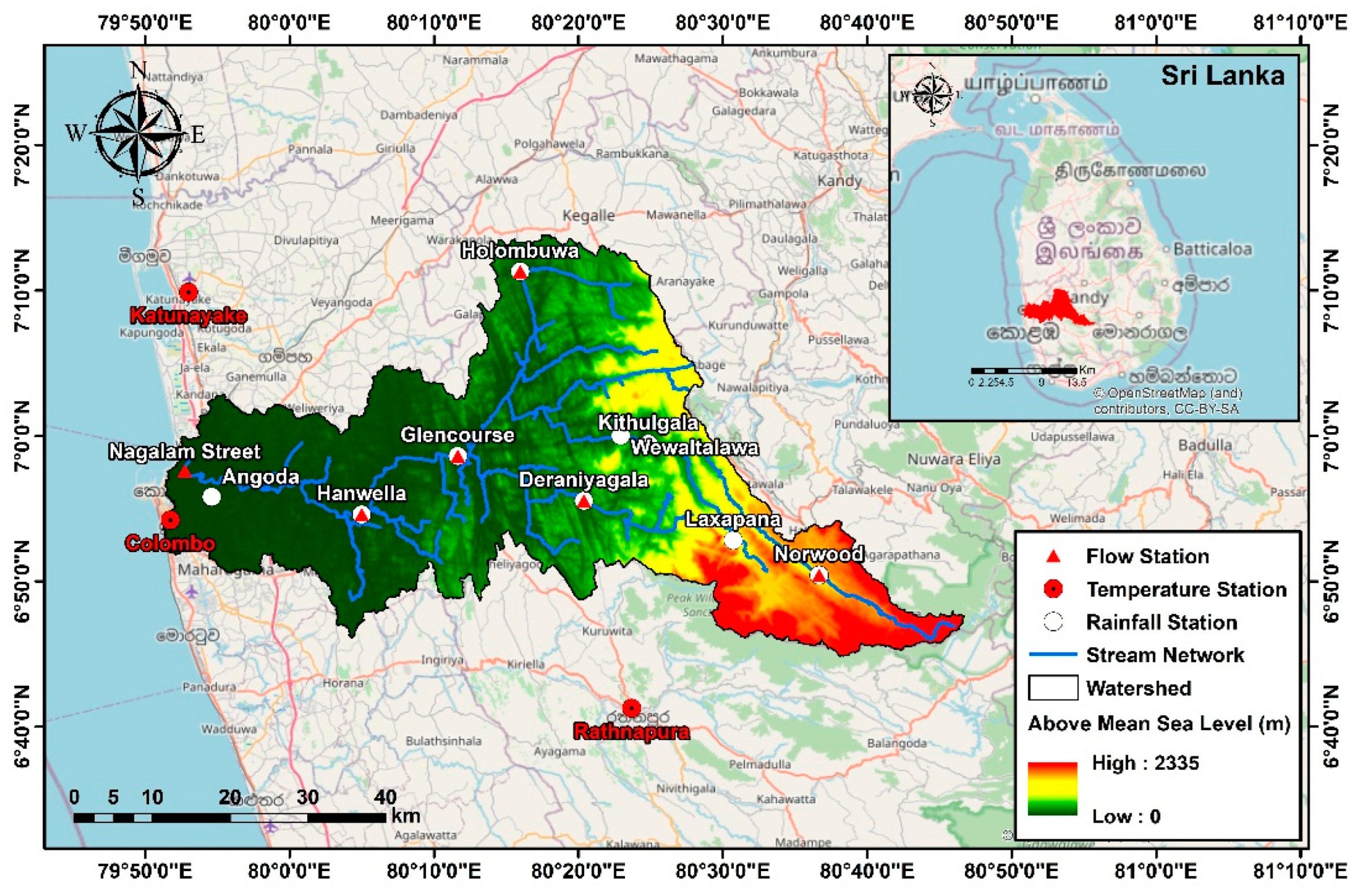
2.1. Study Area

The Kelani River Basin stretches for 145 km and starts from Adam’s Peak Mountains in the island’s central hills. The focus basin in the present work extends approximately 2230 km² (which is slightly lower than the total catchment area of the KRB) discharging to the Indian Ocean in the Kelaniya area, a suburb in the Colombo District. Upstream of the river basin is green with forest, whereas the land use in the downstream part mainly comprises rubber plantations, homestead gardens, and built-up areas. The soil in the study region inherits a loamy nature characterized by low infiltration rates [39].

Figure 1 presents the topography of KRB with the selected meteorological stations (rain gauges and temperature gauges) and flow gauges. The river basin can be divided topographically into upper and lower basins. The upper basin is located upstream of the Hanwella River gauging station and spans approximately 1740 km², while the lower basin is located downstream of Hanwella and covers about 500 km². The lower basin is heavily urbanized, whereas the upper basin is mainly covered with dense vegetation such as tea, rubber, coconut, and forest [40]. The river discharges vary from 800 to 1500 m³/s during monsoon seasons, whereas it falls to 20 to 25 m³/s in the dry season, depending on the operation of three reservoirs in the catchment [41].

2.2. Soil and Water Assessment Tool (SWAT) Model

The Soil and Water Assessment Tool (SWAT) is a river basin model which was developed by the Agricultural Research Service (ARS) of the United States Department of Agriculture (USDA). The model can be used to assess the temporal and spatial behavior of flow situations in rivers. SWAT was initially used to analyze the impact of land uses and land management strategies on water, sediment, and chemical yields in complex watersheds [42]. It helped to work on extended and long-term analysis. SWAT is widely used globally and is considered an adaptable model that can incorporate a variety of environmental processes to enhance more efficient watershed management and the formation of more informed policy decisions [43]. SWAT divides a watershed into sub-watersheds, each further subdivided into hydrologic response units (HRUs) comprised of land use, land management, and soil characteristics [42]. Equation (A1) (in Appendix A) presents the mathematical formulation of SWAT which is based on the water balance.

2.3. SWAT Input Data

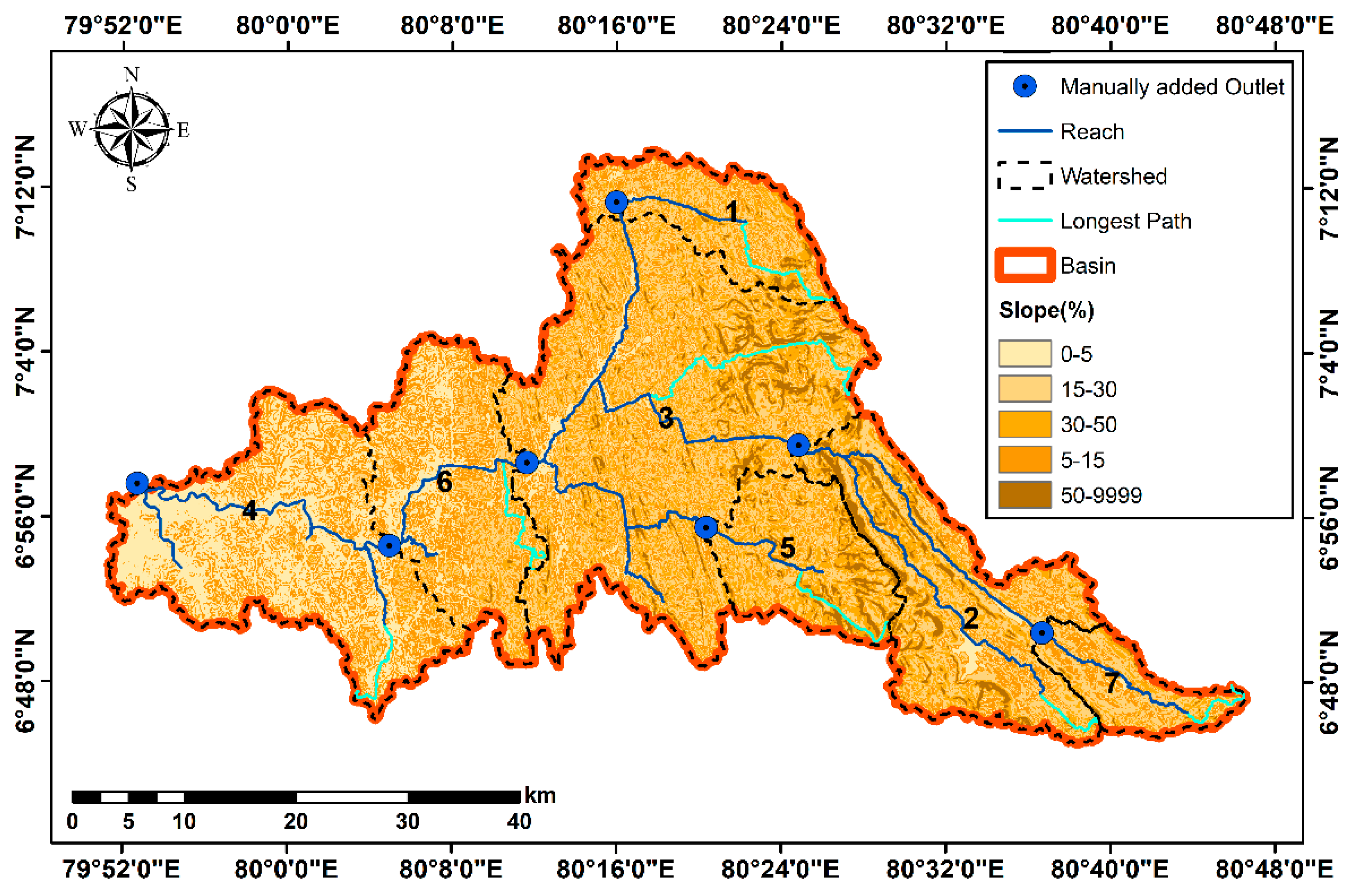
2.3.1. Digital Elevation Model (DEM)

The Kelani River Basin’s watershed boundaries, stream network, topography, and sub-basins with sub-basin characteristics such as slope and slope length were defined using a digital elevation model (DEM) with a 30 m resolution. The resolution of the DEM is a crucial consideration when choosing a DEM for a SWAT model, as it has a considerable impact on the total length of the streamline, the slope of the main channel, the watershed area, and the delineation of the area slope. Buakhao and Kangrang [44] completed a comprehensive analysis of this topic in the application of SWAT modeling and more information can be found in the related reference.

2.3.2. Land-Use Land-Cover (LULC) Properties

The field observation data and high-resolution satellite images from Google Earth were used to perform the land-use land-cover (LULC) classification. Landsat images with a resolution of 30 m × 30 m were used for classification. The image (Satellite Name: Landsat 5, Sensor ID: TM, Acquisition Date: 7 February 1997 and Path/Row: 141/055) retrieved from the United States Geological Survey (USGS) Earth Explorer (https://earthexplorer.usgs.gov/ accessed on 5 September 2022) had a cloud cover of 8.0%. In order to categorize the land into five distinct categories, the land-use classification system developed by the United States Geological Survey (USGS) was used. More information on the USGS classification system can be found in Anderson et al. [45].

Semi-automated classification plugin in QGIS 3.10 was used for the classification. QGIS is considered one of the most common and globally accepted open-source GIS applications. In addition, the training areas and pixel-based image classification were used to perform supervised classification. More information on this open-source toolbox can be found in Congedo [46]. Then, standard training samples were used to classify each land-use class following Lillesand et al. [47]. In addition, the QGIS semi-automatic classification plugin was utilized to evaluate land-cover classification accuracy. Stratified random points (a new function in SCP 6.4.0) were used in the SCP function to generate Region of Interests (ROIs), which were then photo-interpreted and used as a reference for the accuracy assessment. The error matrix and estimated accuracy values were then developed by the SCP Accuracy tool.

There are a variety of approaches for determining the appropriate sample size and distribution in these types of studies. As a general rule, random sampling is the most effective method for ensuring low estimates of standard errors in accuracy. The proportions of land cover classes and the standard errors that were anticipated for overall land cover categorization and individual classes significantly impact the sample design. Class-specific estimations can be improved by stratifying the sample. Olofsson et al. [48] provided further information on sample size and stratification. The sample size ($N$) can be computed as per Equation (1).

$$N={\left({\displaystyle \sum }_{i=1}\frac{W_i\times S_i}{S_0}\right)}^2$$

(1)

where $W_i$ is the class $i$ area to total area (proportion); $S_i$ is the standard deviation of $i$ stratum; $S_0$ is the standard deviation expected for overall accuracy.

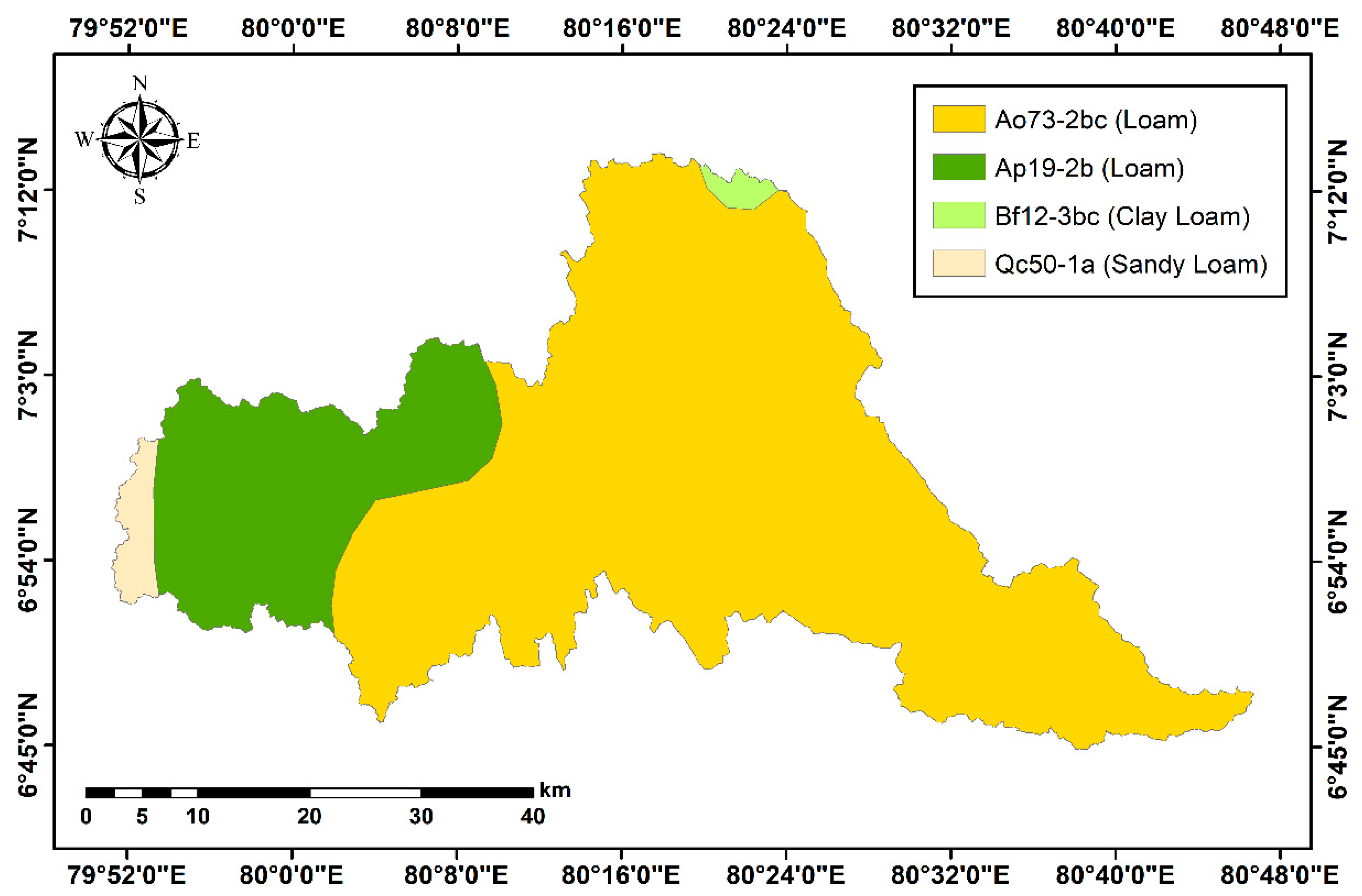
2.3.3. Soil Properties

The soil properties of KRB were derived from the Food and Agriculture Organization (FAO) and The United Nations Educational, Scientific and Cultural Organization (UNESCO) soil maps. Four major soil types, loam, clay, and sandy soils (refer to

Table 1. Soil classification and description.

Soil Name	Texture	Hydrological Soil Group	Area (km2)
Ao73-2bc-3645	Loam	C	1810.7
Ap19-2b-3654	Loam	C	467.2
Qc50-1a-3841	Sandy Loam	C	41.4
Bf12-3bc- 3687	Clay Loam	C	15.5

) can be identified as per the SWAT global soil database.

The soil map for the KRB is given in Figure 2. The spatial variation of soil types can be clearly seen in this figure. The upstream of the KRB mostly has Ao73-2bc-3645 soil whereas the downstream has both clay and sandy loam soils.

2.3.4. Meteorological and Hydrological Data

Daily resolution meteorological data of rainfall, minimum and maximum temperature, relative humidity, solar radiation, and wind speed data have to be fed to the SWAT model. These data can either be ground measured or generated by the SWAT WXGEN weather generator. This weather generator helps to fill the gaps in ground-measured data [49]. Sri Lanka has widespread rainfall measuring stations; however, it only has a few temperature and other meteorological data measuring stations (less than 25 for the whole country). Therefore, observed rainfall and temperature data were used in modeling; however, due to lack of measured data, the relative humidity, wind speed, and solar radiation data from 1994 to 2015 were generated. The daily rainfall data of Laxapana, Hanwella, Wewalthalawa, Norwood, Kitulgala, Holombuwa, Deraniyagala, Glencourse, and Angoda, and temperature data of Colombo, Katunayake, and Rathnapura were purchased from the Department of Meteorology, Sri Lanka, from 1994 to 2015. These gauging stations are shown in Figure 1. In addition, daily discharge data for five flow stations, including Hanwella, Glencourse, Kitulgala, Holombuwa, and Deraniyagala, were purchased from the Department of Irrigation, Sri Lanka. These data were used to conduct the sensitivity analysis first and then to calibrated and validate the SWAT model.

2.4. Detailed Analysis

2.4.1. Watershed Delineation and Hydrological Response Units (HRUs)

This study used ArcGIS 10.4.1 and the 2012 version of SWAT (which can be downloaded from http://swat.tamu.edu/software/ accessed on 5 September 2022) computer modules for in-depth analysis. Initially, the input raster files (DEM, soil map, and LULC map) were all projected into the same geographic coordinate system (i.e., UTM zone 44N for Sri Lanka). Generally, the watershed delineation procedure consists of establishing a DEM, defining streams, inlets, and outlets, and calculating sub-basin parameters. The in-stream definitions process was not defined correctly by the ArcSWAT model and was not delineated through the Glencourse flow station. To address the issue with stream definitions, this study used the SAGA tool combined with the open street map (OSM) plugin in QGIS 3.10. The stream was burned to ArcSWAT after the river network was derived by identifying the Strahler order. A catchment boundary with a total area of 2239.5 km² was recognized by the model.

This KRB was subdivided into seven sub-basins with manually added outlets. After that, the land area of each sub-basin was split into hydrological response units (HRUs). Fifty-three HRUs were identified. The slope map, soil layers, and LULC were imported into the project using ArcSWAT’s HRU analysis tool. Thus, the land use and soil layers have completely enclosed the delineated watershed. In addition to land use and soils, SWAT HRU analyses have included classifications of HRUs by slope classes; therefore, the multiple slope option was selected. After reclassifying the LULC, slope, and soil maps to correspond with SWAT database values, these physical attributes were overlaid to define the HRUs. In this study, the threshold values of 15%, 5%, and 5% were specified for land use, slope, and soil, respectively, for analysis.

2.4.2. Parameter Selection

The SWAT flow simulation was performed with monthly frequency after processing the required inputs from 1994 to 2015. The initial three years (1994 to 1996) were allocated to warm up the model. The SWAT model was performed with the default SWAT parameters during the simulation. Relevant SWAT parameters, including the baseflow alpha-factor (ALPHA BF.gw), the minimum water level required for the formation of baseflow (GWQMN.gw), the time needed for water to reach the shallow aquifer after leaving the root zone (GW DELAY.gw), the groundwater re-evaporation coefficient (GW_REVAP), the curve number (CN2.mgt), the threshold depth at which water can percolate from the shallow aquifer into the deeper aquifer (REVAPMN), the compensation factor for the soil evaporation (ESCO.hru), and the maximum canopy water storage (CANMX.hru) were selected by the literature and visual observations of both observed and simulated hydrographs. Overestimations, underestimations, and deviations in the discharge graphs were highlighted.

Before the manual calibration, a SWAT-CUP analysis was carried out to identify the most sensitive parameters. SWAT-CUP is an independent program designed for SWAT calibration [50]. Five distinct calibration processes (Particle Swarm Optimization (PSO), Markov Chain Monte Carlo (MCMC), Sequential Uncertainty Fitting ver.2 (SUFI-2), Generalized Likelihood Uncertainty Estimation (GLUE), and Parameter Solution (Parasol)) are included in the program, as well as functions for validation and sensitivity analysis and a Bing map visualization of the study area. As part of the SWAT-CUP analysis, this study adopted the Latin Hypercube Sampling technique from the SUFI-2 to calibrate and estimate uncertainty [50,51]. The SUFI-2 algorithm is the most common and computationally efficient method, having the best P-factor (prediction uncertainty ranges) and R-factor (relative coverage of measurements) compared to other methods [38,52,53,54].

2.4.3. Calibration and Validation

Calibration optimizes the model output by modifying or adjusting the model parameters within the allowed limits to correspond with the observed data. The values of these parameters can be altered either manually or automatically so that the predicted results are in close enough accordance with the observed data. In this study, the SWAT model was manually calibrated for twelve years (1997–2008) and validated for seven years (2009–2015), with three years serving as a warmup period (1994–1996).

Even though there were seven outlets in the basin, only five were considered for the analysis. The fourth outlet, Nagalagam Street, is the closest outlet to the sea and is therefore subject to tides [54]. Consequently, it was not possible to observe or simulate the discharge, and outlet number 4 cannot be used (fourth sub-basin). In addition, the discharge data from Norwood (outlet 7) were inadequate for the analysis. The remaining outlets (refer to Figure 3) were calibrated and validated. The research included two calibration methods, single-site calibration and multi-site calibration.

In single-site calibration, the authors used the upstream station (Deraniyagala) and the downstream station (Hanwella) and calibrated each case independently. The resulting sub-basin parameter values were then assigned to the remaining four sub-basins. Multi-site calibration was accomplished by calibrating from the upstream to the downstream river while holding identical values for each sub-basin.

2.4.4. Performance Evaluation of the Model

The performance of the model was evaluated using statistical indices such as the Nash–Sutcliffe model efficiency (NSE), the RMSE-observations standard deviation ratio (RSR), the percentage of bias (PBIAS), and the coefficient of determination ($R^2$) (find the equations and definitions in Appendix B). The $R^2$ ranges between 0 and 1 and measures the model’s ability to explain the variance of observed data. The greater the number, the lower the error variance of the model, and vice-versa for lower numbers. Generally, $R^2$ > 0.5 is considered the acceptable range for a model [55,56]. The mathematical formulation for $R^2$ is given in Equation (A2).

The Nash–Sutcliffe efficiency (NSE) is a normalized statistic that evaluates the amount of residual variance relative to the variance of observed data and reflects the fit between simulated and observed data plots [57]. While Servat and Dezetter [58] state that the NSE is the best objective function to reflect the overall fit of a hydrograph, Legates and McCabe Jr [59] recommend using the NSE. When it is set to 1, the output is optimal. In general, models with an NSE of at least 0.5 are considered to be in acceptable form. The mathematical formulation of the NSE is given in Equation (A3).

Based on the recommendations of Singh et al. [60], the RMSE-observations standard deviation ratio (RSR) is computed as the ratio between the RMSE and the standard deviation of measured data. Root-mean-squared error (RMSE) is one of the most often employed error-index statistics [60,61]. Error-index statistics and a scaling/normalization factor make it possible to apply the final statistic and reported values to various constituents. With an RSR value between 0 and $\infty$, which shows 0 RMSE or residual variation and thus perfect model simulation, the RSR spans from 0 to a significant positive value. This produces a low RSR and decreased RMSE, which in turn improves model simulation outcomes. Equation (A4) presents the mathematical formulations of the RMSE-observation standard deviation ratio.

The percent bias (PBIAS) measures the average tendency of simulated data to differ from their observed counterparts in terms of percentage (refer to Equation (A5)). For example, a model with a negative PBIAS indicates overestimation, whereas a positive PBIAS indicates underestimating. PBIAS is frequently used to measure water balance errors and has the capability to reveal poor model performance [62]. During dry seasons, PBIAS values for streamflow tend to vary more among different autocalibration methods than in wet seasons [62].

Table 2. Model performance evaluations for monthly discharge simulation [63,64,65].

Indices	R2	NSE	RSR	PBIAS
Range	0 to 1	$-\infty$ to 1	$0$	$-\infty$ to $\infty$
Optimal Value	1	1	0	0
Satisfactory Value	>0.5	>0.5	≤0.7	<±25

presents the summary of performance evaluation values for monthly discharge simulations, which were recommended by many researchers.

3. Results and Discussion

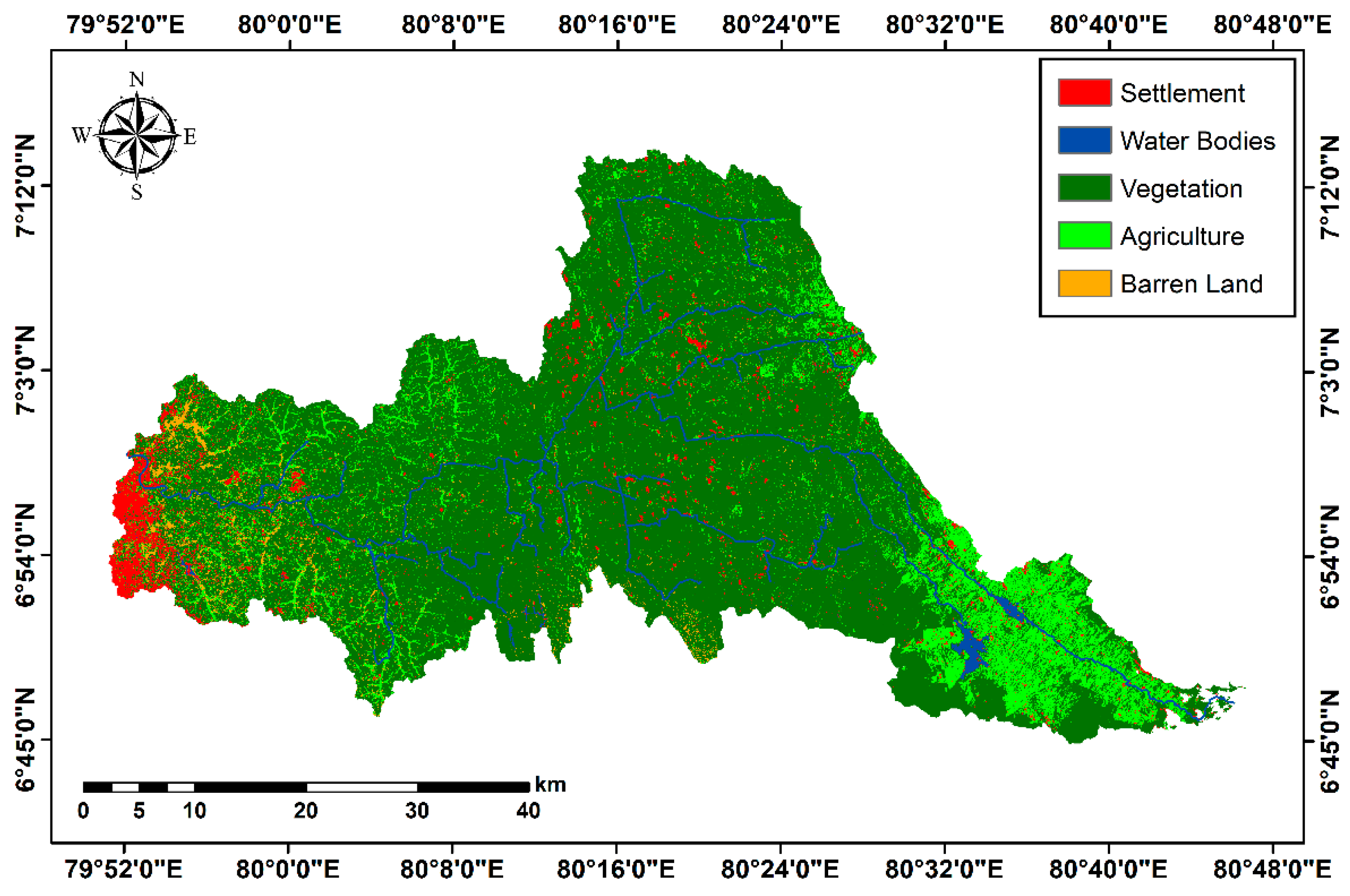
3.1. Land-Use Land-Cover Classification

The classification accuracy was examined using the Kappa coefficient and was above 81%, while the overall classification accuracy was over 84%, suggesting that the classification was acceptable for the analysis. Forest land area (1875.8 km²) was the highest in 1997, while the water bodies (16.9 km²) acquired a small percentage of the area in the Kelani River Basin. However, agricultural lands shared a significant percentage while more settlements can be seen downstream of the KRB. Figure 4 showcases the land use land cover for KRB in 1997. Other assessed land cover is given in

Table 3. Land-use classes in Kelani River Basin (in 1997) and corresponding SWAT codes.

Land Use	SWAT Land-Use Class		Area (km2)
	Model Code	Description
Settlements	URBN	Urban	91.3
Agriculture	AGRL	Agricultural Land-Generic	302.3
Forest	FRST	Forest-Mixed	1875.8
Barren lands	BARR	Barren	38.6
Water bodies	WATR	Water	16.9

with their areas.

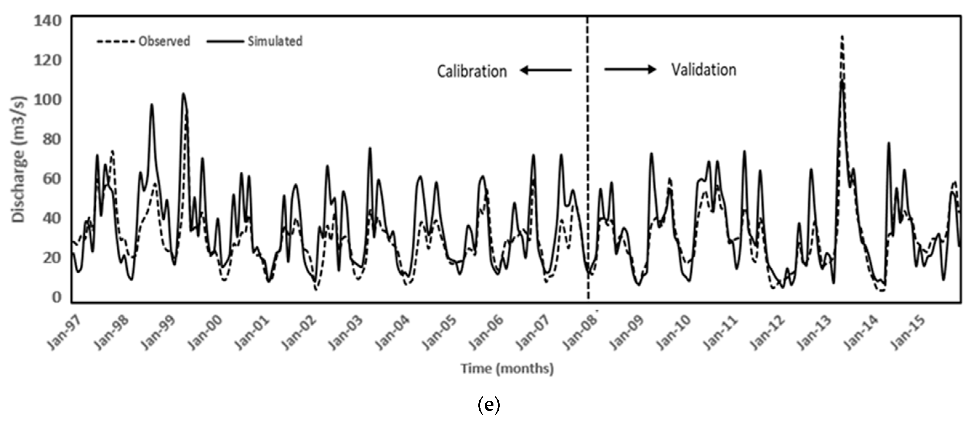
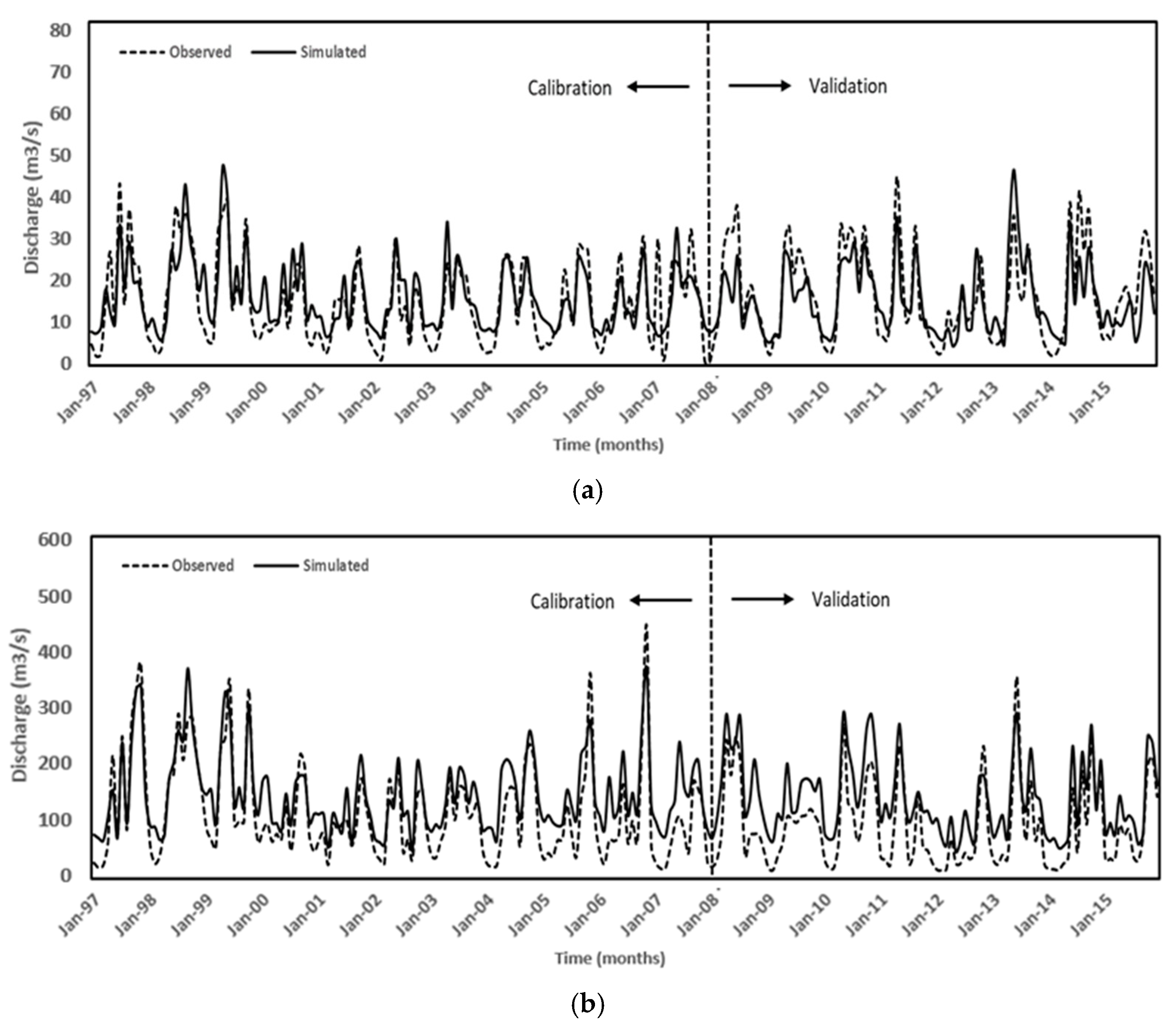
3.2. Single-Site Calibration and Validation

3.2.1. Hanwella Sub-Basin

Initially, the SWAT model was calibrated using downstream data (Hanwella sub-basin), and the obtained values for the selected parameters were then assigned to other basins as is customary with the single-site calibration technique. Figure 5 showcases the calibration and validation of observed and simulated streamflows. The streamflow gauges Hanwella, Deraniyagala, Glencorse, Holombuwa, and Kithulgala illustrate a good agreement between observed and simulated streamflow data, highlighting a good performance of the model, while slight overestimations are seen at Glencorse and Kithulgala stations and slight underestimation can be observed during some of the months of 1997, 1998, 2010, and 2015 at Kithulgala station (refer to Figure 5c,e).

Throughout the calibration period, the model performances for Hanwella, Deraniyagala, and Holombuwa stations were deemed “good” with the indices RSR and NSE, values of (0.6, 0.65), (0.52, 0.66), and (0.56, 0.72), respectively (refer to

Table 4. Performance evaluations for the monthly discharge simulation (Hanwella sub-basin).

Station	${\mathit{R}}^2$	NSE	PBIAS	RSR	${\mathit{R}}^2$	NSE	PBIAS	RSR
	Calibration				Validation
Hanwella	0.82	0.65	−29.34	0.6	0.85	0.51	−43.94	0.75
Deraniyagala	0.69	0.66	−3.9	0.52	0.69	0.62	5.97	0.53
Glencorse	0.81	−0.96	-81.94	1.58	0.69	−0.17	−40.75	1.05
Holombuwa	0.73	0.72	−4.24	0.56	0.61	0.59	0.34	0.60
Kithulgala	0.61	−0.07	−20.35	1.05	0.7	0.59	−7.58	0.59

). In addition, the PBIAS stayed less than ±10 at Deraniyagala and Holombuwa stations, and the model performance was assessed as “very good”. However, the PBIAS ≥ 25 at Hanwella station was classified as “unsatisfactory”. Although Kithulgala station shows a “satisfactory” condition with a PBIAS value of (−20.35), the model performance at Glencorse and Kithulgala is rated as “unsatisfactory” for all the statistical indices except $R^2$. Overestimation of the peak flows could be the reason for low NSE values at Glencorse and Kithulgala stations because of the sensitivity of NSE to higher values resulting from squared differences in its derivation. The $R^2$ values ranged from 0.61 to 0.82, suggesting “very good” (0.75–0.89) to “good” (0.50–0.74) performance of the model [66].

During the validation period, model performance was “satisfactory”, with NSE values ranging from 0.51 to 0.62 for all stations except Glencorse (−0.17), which can be rated as “unsatisfactory”. The PBIAS and RSR can be classified as “very good” and “good” for Deraniyagala (5.97, 0.53), Holombuwa (0.34, 0.6), and Kithulgala (−7.58, 0.59), whereas Hanwella (−43.94, 0.75) and Glencorse (−40.75, 1.01) are evaluated as “unsatisfactory”. $R^2$ varies from 0.61 and 0.85, signifying “very good” (0.75–0.89) to “good” (0.50–0.74) model performance.

Table 5. SWAT model calibrated parameters (Hanwella sub-basin).

Parameter	Description of the Parameter	Fitted	Min	Max
ALPHA_BF.gw	Alpha-factor of the baseflow in days	0.9998	0	1
GW_DELAY.gw	Groundwater lag time in days	146.45	0	500
GWQMN.gw	In a shallow aquifer, the threshold water depth is needed for the return flow (mm)	325	0	5000
GW_REVAP	Groundwater “revap” coefficient	0.1985	0.02	0.2
REVAPMN	The threshold depth at which water can percolate from the shallow aquifer into the deeper aquifer (mm)	175	0	500
CN2.mgt *	Runoff curve number	Varied	35	98
CANMX.hru	Canopy water storage (maximum) (mm)	84.356	0	100
ESCO.hru	Compensation factor of soil evaporation	0.985	0.01	1

* CN2.mgt values were varied with the land use (forest: 80, settlements: 90, agriculture: 80, water bodies: 92, bare lands: 80).

showcases the model calibrated parameters for Hanwella sub-basin and these values can be effectively used in any future study.

3.2.2. Deraniyagala Sub-Basin

Figure 6 presents the calibration and validation results for the Deraniyagala sub-basin. Similar to the initial single-site calibration approach, the simulated flow at Hanwella, Deraniyagala, Glencorse, Holombuwa, and Kithulgala gauging stations showed a good fit with observed data, with a slight overestimation of the flow at Glencorse and Kithulgala for the majority of the years of the studied period (refer to Figure 6c,e).

In the calibration period, the model performances at Deraniyagala and Holombuwa stations were graded as “good” based on the NSE and RSR indices (0.66, 0.56) and (0.69, 0.57), respectively. In addition, Hanwella (0.65, 0.64) was rated “good” for the NSE and “satisfactory” for the RSR, while Kithulgala (−0.07, 1.06) was deemed “unsatisfactory” for both indices (refer to

Table 6. Performance evaluations for the monthly discharge simulation (Deraniyagala sub-basin).

Station	${\mathit{R}}^2$	NSE	PBIAS	RSR	${\mathit{R}}^2$	NSE	PBIAS	RSR
	Calibration				Validation
Hanwella	0.81	0.65	−29.26	0.64	0.84	0.41	−51.41	0.87
Deraniyagala	0.66	0.66	−4.77	0.56	0.69	0.68	6.06	0.55
Glencorse	0.8	−0.87	−81.89	1.58	0.66	−0.15	−41.99	1.06
Holombuwa	0.72	0.69	−3.16	0.57	0.58	0.57	0.06	0.6
Kithulgala	0.56	−0.07	−20.79	1.06	0.64	0.55	−7.96	0.62

). The PBIAS at Deraniyagala and Holombuwa stations did not surpass ±10; hence they were assessed as “very good.” Hanwella and Kithulgala were rated as “unsatisfactory” and “satisfactory” for the PBIAS, whereas Glencorse was rated as “unsatisfactory” for all indices except $R^2$, as is customary. $R^2$ values ranged from 0.56 to 0.81, suggesting “very good (0.75–0.89)” to “good (0.50–0.74)” performance of the model.

The model performance for the validation period was “unsatisfactory” for the NSE, PBIAS, and RSR indices at Hanwella (0.41, −51.41, 0.87) and Glencorse (−0.15, −41.99, 1.06) stations. However, the values of PBIAS for Deraniyagala (6.06), Holombuwa (0.06), and Kithulgala (−7.96) stations were less than ±10, which indicates a “very good” model performance. The NSE and RSR indices demonstrated “good” performance at the Deraniyagala (0.68, 0.55) and “satisfactory” performance at the Kithulgala (0.55, 0.65) stations. Holombuwa’s model performance with RSR was deemed “good”, whereas the NSE suggests a “satisfactory” performance. $R^2$ indicates that the model performance at all stations falls within the range of “very good” (0.75–0.89) to “good” (0.50–0.74). Detailed analyses of these results are given in Table 6. Similar to the Hanwella sub-basin,

Table 7. SWAT model calibrated parameters (Deraniyagala sub-basin).

Parameter	Description of the Parameter	Fitted	Min	Max
ALPHA_BF.gw	Alpha-factor of the baseflow in days	0.9998	0	1
GW_DELAY.gw	Groundwater lag time in days	340	0	500
GWQMN.gw	In a shallow aquifer, the threshold water depth is needed for the return flow (mm)	320	0	5000
GW_REVAP	Groundwater “revap” coefficient	0.1965	0.02	0.2
REVAPMN	The threshold depth at which water can percolate from the shallow aquifer into the deeper aquifer (mm)	180	0	500
CN2.mgt*	Runoff curve number	Varied	35	98
CANMX.hru	Canopy water storage (maximum) (mm)	84.356	0	100
ESCO.hru	Compensation factor of soil evaporation	0.985	0.01	1

* CN2.mgt values were varied with the land use (forest: 80, settlements: 90, agriculture: 80, water bodies: 92, bare lands: 80).

presents the calibrated parameters for SWAT model for Deraniyagala sub-basin. These calibrated values can be used in any future study.

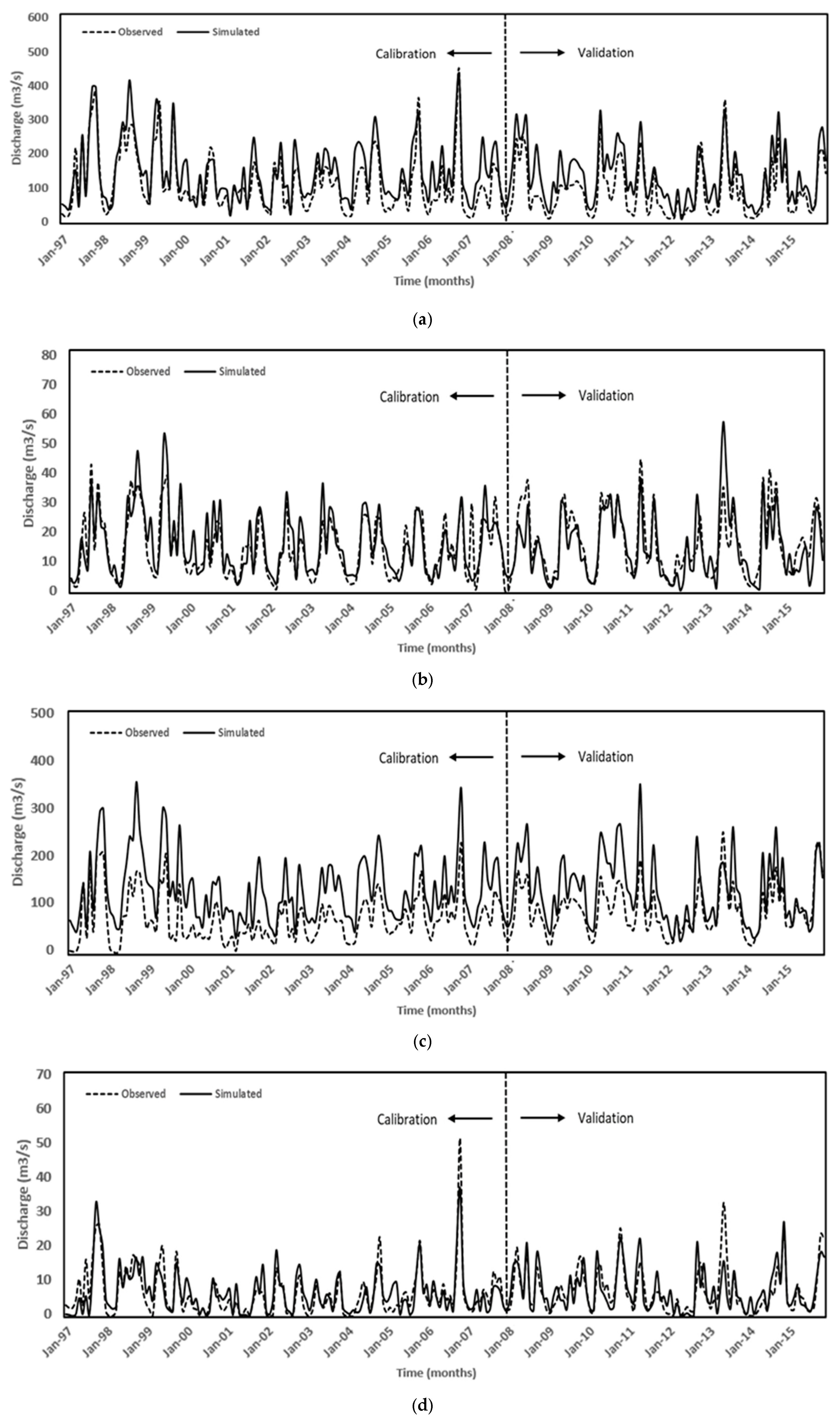
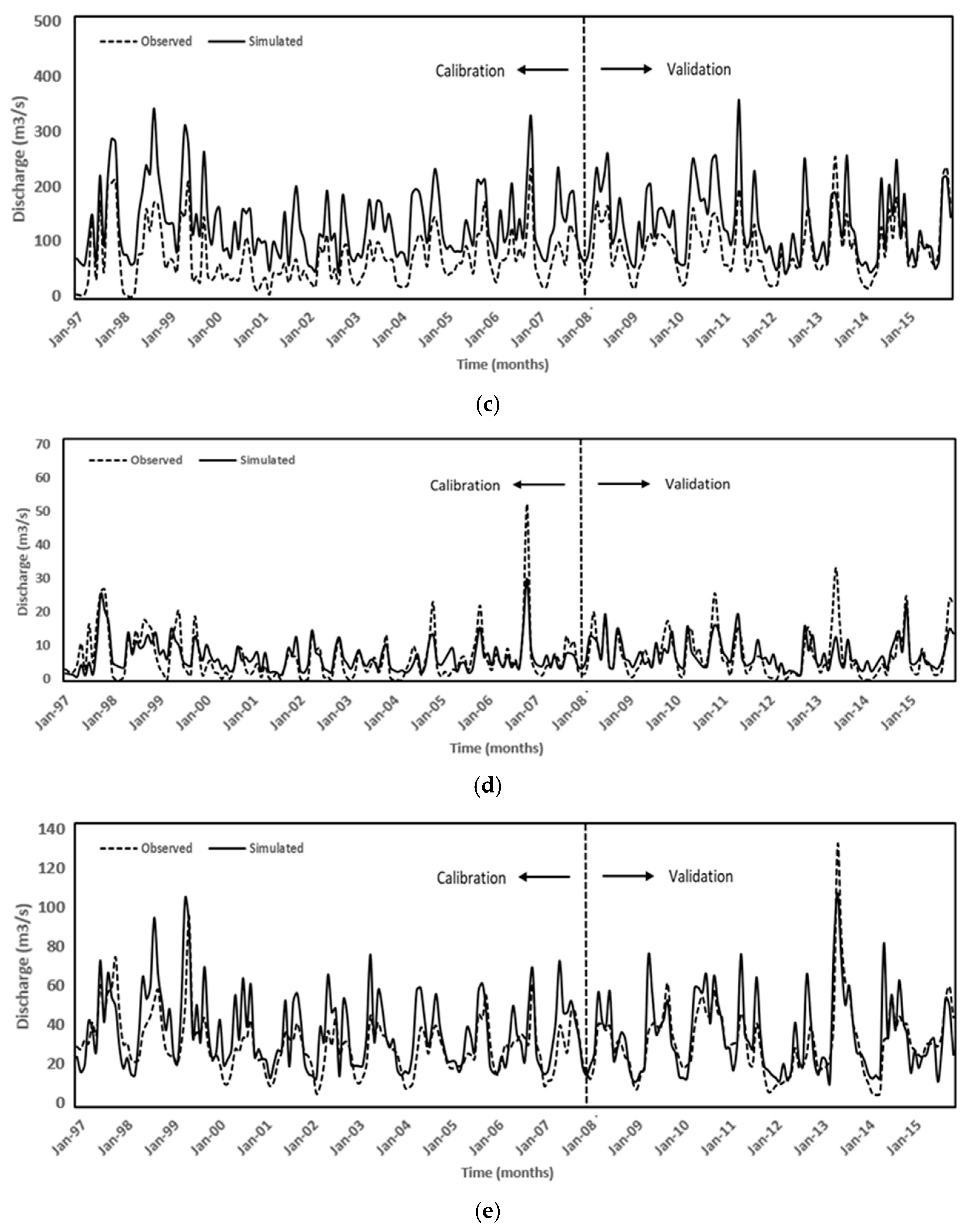
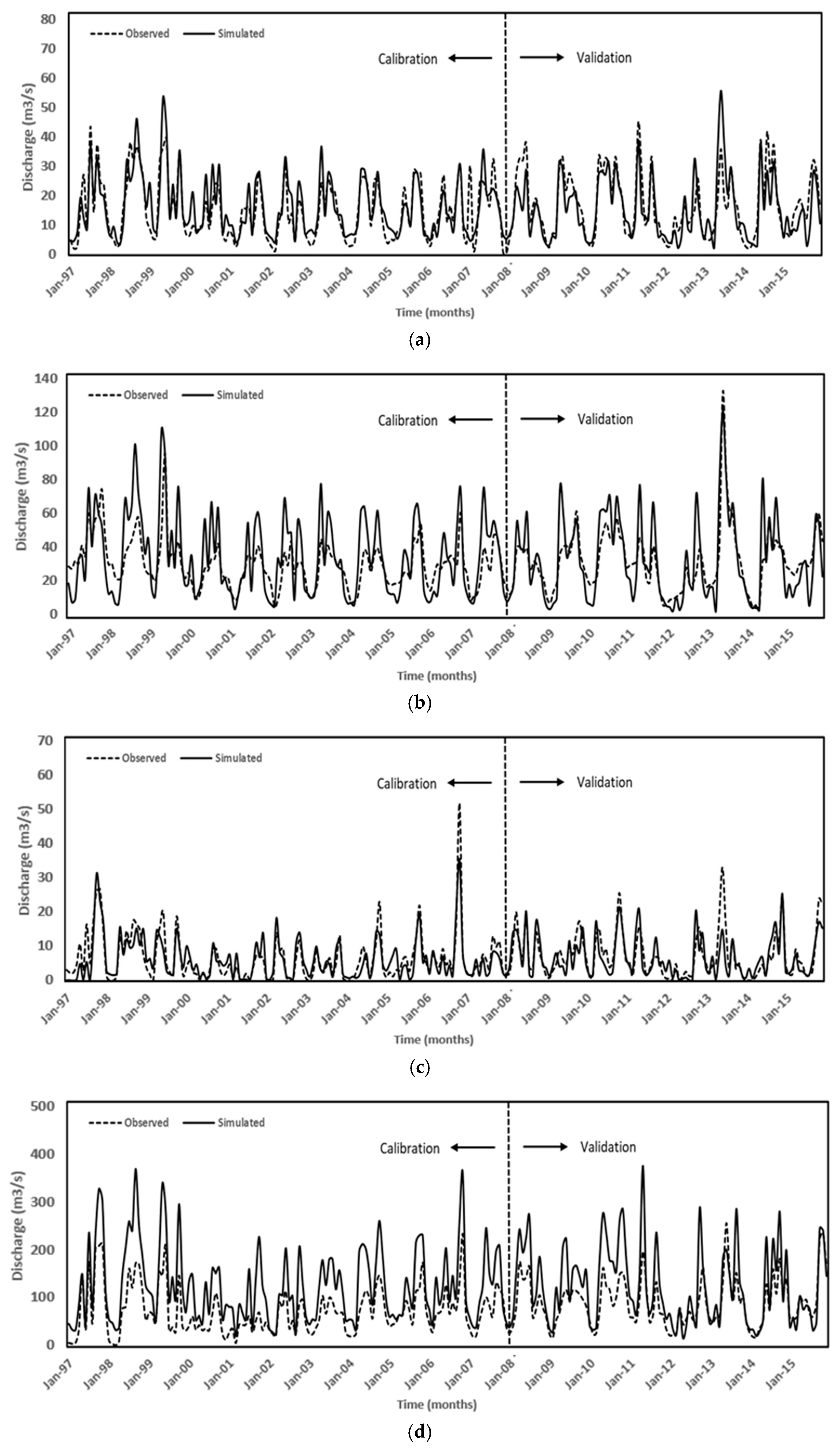
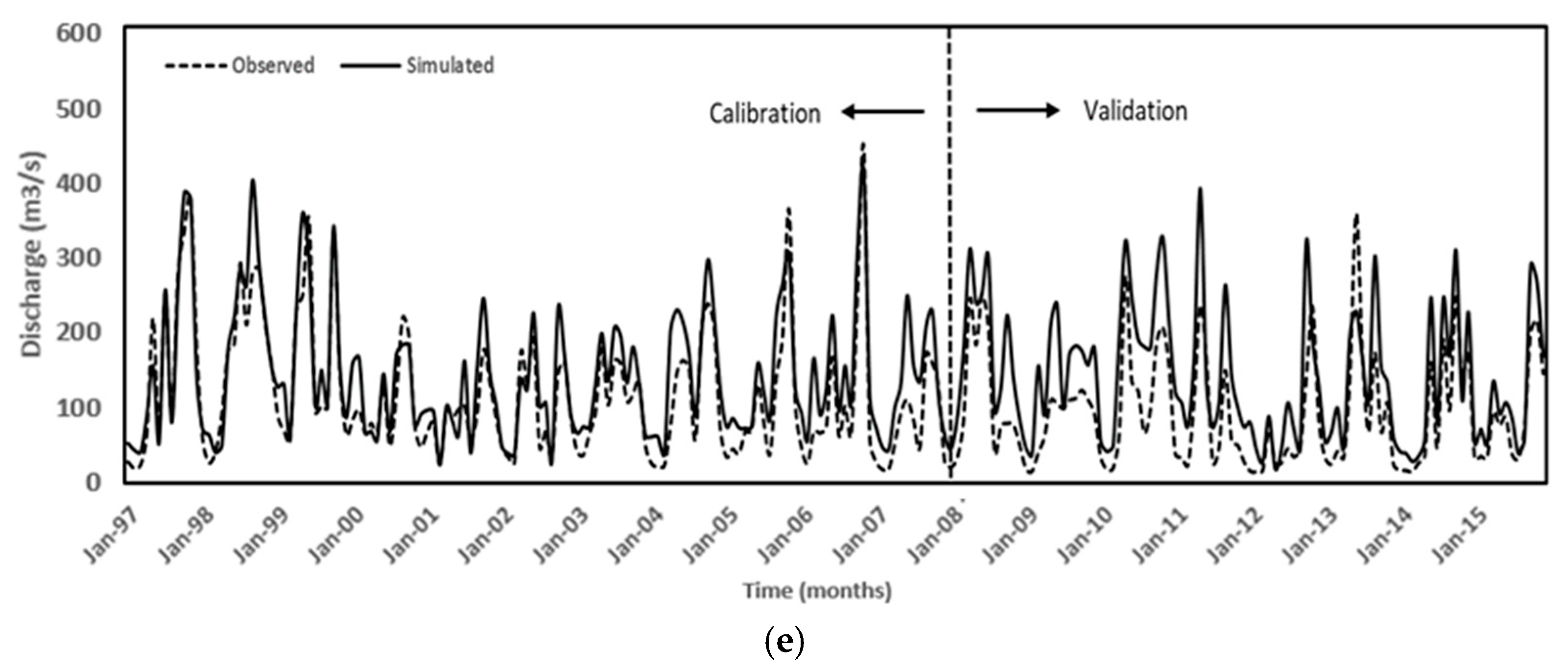
3.3. Multi-Site Calibration and Validation

Figure 7 presents the results for multi-site calibration and validation. In multi-site calibration, an excellent fit was witnessed with the observed discharges for all the stations, with a slight underestimation during the years 1997 to 1999, 2005 to 2006, 2010 to 2013, and 2015, and an overestimation during the remaining years, except a few months at the Kithulgala station and a slight overestimation at the Glencorse station, similar to the initial single-site calibration approach (refer to Figure 7b,d).

The model performance for the Hanwella was assessed as “very good” based on the $R^2$ for both calibration and validation periods (refer to

Table 8. Performance evaluations for the monthly discharge simulation.

Station	${\mathit{R}}^2$	NSE	PBIAS	RSR	${\mathit{R}}^2$	NSE	PBIAS	RSR
	Calibration				Validation
Hanwella	0.83	0.71	−23.67	0.53	0.82	0.51	−40.68	0.73
Deraniyagala	0.68	0.66	−4.34	0.50	0.70	0.66	5.77	0.51
Glencourse	0.81	−0.87	−72.75	1.41	0.69	−0.28	−34.16	0.99
Holombuwa	0.75	0.75	5.09	0.52	0.61	0.59	9.51	0.58
Kithulgala	0.59	−0.32	−13.51	1.17	0.69	0.50	−1.79	0.69

). The NSE and RSR indices exhibited “good” performance of the model within the calibration period, whereas the PBIAS was “satisfactory”. However, throughout the validation period, the PBIAS and RSR evaluated the model performance in Hanwella as “unsatisfactory”, although the NSE rated it as “satisfactory”. In addition, the Deraniyagala sub-basin outperformed all other sub-basins, with all model performance indices falling within the range of “very good” and “good” for both calibration and validation periods. Holomabuwa follows a similar trend, except that the NSE graded the model’s performance as “satisfactory” during the validation period.

Furthermore, the model performance of Glencorse was graded as “unsatisfactory” by all indices except $R^2$, which indicated a “very good” and “good” model performance for both calibration and validation, respectively. In the calibration period, model performance for the Kithulgala sub-basin was assessed as “good” based on the the $R^2$ and PBIAS indices. However, during the validation period, model performance was rated as “good” for both indices except the PBIAS, which increased to “very good” performance. NSE and RSR ranked the model performance as “unsatisfactory” and “good” in calibration and validation periods, respectively.

Table 9. Fitted values for calibrated model parameters.

Parameter Name	Station
	Hanwella	Deraniyagala	Glencourse	Holombuwa	Kithulgala
ALPHA_BF.gw	0.9998	0.9998	0.9998	0.9998	0.9998
GW_DELAY.gw	146.45	340	340	340	120
GWQMN.gw	325	320	320	320	320
GW_REVAP	0.1985	0.1965	0.1965	0.1965	0.1995
REVAPMN	175	180	180	180	175
CN2.mgt *	Varied	Varied	Varied	Varied	Varied
CANMX.hru	84.356	84.356	84.356	84.356	99.356
ESCO.hru	0.985	0.985	0.005	0.485	0.005

* CN2.mgt values were varied with the land use (forest: 80, settlements: 90, agriculture: 80, water bodies: 92, bare lands: 80).

presents the fitted values for SWAT calibrated values. As it was presented under Table 5 and Table 7, these calibrated values can be effectively used by any future study for the same catchment.

3.4. Comparative Analysis

The average annual basin values from a single-site and multi-site calibration were obtained for comparative analysis and shown in

Table 10. Average annual basin values.

Variable Name	Description	Single-Site Calibration		Multi-Site Calibration
		Calibration 01	Calibration 02
Precip	Watershed average precipitation used in the simulation (mm)	3897.6	3897.6	3897.6
Surface Runoff Q	Simulation-based surface runoff generated in the watershed (mm)	1501.3	1080.1	1520.8
Lateral Soil Q	Simulated lateral flow contribution to streamflow in the watershed (mm)	130.7	179.6	131.9
Groundwater (Shal Aq) Q	Simulated groundwater flow into the watershed’s stream (mm) (shallow)	664.7	1023.4	669.3
Groundwater (Deep Aq) Q	Simulated groundwater flow into the watershed’s stream (mm) (deep)	51.7	70.4	48.3
Revap (Shal Aq => Soil/Plants)	Amount of water simulated to flow from a shallow aquifer to the watershed’s vegetation and soil profile (mm)	318.1	313.7	249.1
Deep Aq Recharge	Simulated deep aquifer recharging in the watershed (mm)	51.7	70.4	48.4
Total Aq Recharge	Calculated flow entering into both watershed aquifers (mm)	1034.9	1407.6	967.4
Total Water Yld	Simulated water yield from HRUs in the watershed (mm)	2348.4	2353.6	2370.4
Percolation Out of Soil	Simulated water percolation at the soil profile’s base in the watershed (mm)	1039.7	1412.4	968.9
ET	Simulated evapotranspiration in the watershed (mm)	1225.6	1225.1	1275
PET	Simulated potential evapotranspiration in the watershed (mm)	1611.4	1611.4	1611.4
Total Sediment Loading	Simulated sediment yield from HRUs in the watershed (metric tons/ha)	111.4	138.2	141.6

. Both single-site calibrations showcase similar range values for average annual values. However, some significant changes can also be seen (surface runoff, groundwater, etc.). This considerable difference may result from the several calibration procedures with varying parameter values. For instance, the GW DELAY.gw values (146.45 and 340) were altered during two calibration operations, as illustrated in Table 5 and Table 7, which can immediately impact the simulated groundwater flow into the watershed’s stream. In addition, the multi-site calibration values are approximately similar to calibration 1 (Hanwella gauging station) from single-site calibration. They do not show much difference. Hanwella gauging station is far downstream compared to the Deraniyagala gauging station, and this could be a reason for having a slightly increased deviation from single-site calibration to multi-site calibration.

The hydrological features of a basin are represented by its annual mean values for both calibration methods. The ratio between precipitation (P) and potential evapotranspiration ($E_p$) reveals the moisture state, which reflects the climate condition of the region. By analyzing this ratio, the climate condition of the relevant study region may be identified, and it may assist the authorities in determining whether the results of this study would accurately reflect the actual setting of the basin. According to the National Oceanic and Atmospheric Administration (NOAA), the relevant climate conditions and the ratio between P and $E_p$ are shown in

Table 11. The ratio between the P and $E_p$ and relevant climate conditions [67].

$\mathbf{Precipitation}/\mathbf{Potential}\mathbf{Evapotranspiration}\left(\mathit{P}/{\mathit{E}}_{\mathit{p}}\right)$	Climate Condition
<0.4	Arid
0.4–0.8	Semi-arid
0.8–1.2	Sub-humid
>1.2	Humid

.

This study indicates a $P/E_p$ value of 2.4 corresponds to expected humid conditions, given that the Kelani River Basin is a tropical watershed. This information is important for validating the remaining hydrological features of the basin.

A few studies on SWAT models in Sri Lanka have been conducted [68,69,70]. Among them, Siriwadana and Rajapakse [37] were the first to document SWAT model results in the Kelani River Basin. The results of our study will guide water resource management authorities in decision making with optimal data availability. Thus, the research work presented herein creates the novelty of the work in the context not only in the KRB but also in a country blessed with more than 100 rivers that are spread all over the country: Sri Lanka.

The results of this analysis incorporate several uncertainties. According to Gunathilaka and Samarasinghe [54,71], the backwater effect from tidal affects up to the Hanwella gauge (which is in the upstream). This can alter the discharge of the river. Moreover, the SWAT model has its own uncertainties. Since the model simulates watershed processes through several assumptions, significant uncertainties are carried out through the model simulation result.

4. Summary and Conclusions

This study evaluates the SWAT model calibration using three distinct calibration procedures, including (1) single-site calibration with downstream data, (2) single-site calibration with upstream data, and (3) multi-site calibration using downstream and upstream data approach for the first time in the context of Sri Lanka. Calibration was performed using SWAT parameters, including the baseflow alpha-factor (ALPHA BF.gw), the minimum water level required for the formation of baseflow (GWQMN.gw), the time needed for water to reach the shallow aquifer after leaving the root zone (GW DELAY.gw), the groundwater “re-evaporation” coefficient (GW_REVAP), the curve number (CN2.mgt), the threshold water level in the shallow aquifer for “re-evaporation” to occur (REVAPMN), the maximum canopy water storage (CANMX.hru), and the soil evaporation compensation factor (ESCO.hru). These parameters were selected by the literature and visual observations of both simulated and observed hydrographs.

The performance of the model was evaluated using statistical indices, including coefficient of determination ($R^2$), the Nash–Sutcliffe model efficiency (NSE), the RMSE observed standard deviation ratio (RSR), and the percentage of bias (PBIAS). These are the most prevalent statistical indices in the literature for evaluating SWAT model performance. The results indicate a satisfactory fit between these calibration approaches (single and multi-site calibration) and the observed data, with a notable improvement in the multi-site calibration strategy compared to the other two methods. The study concluded that, although the multi-site calibration strategy requires a considerable amount of time, the accuracy of the results can be improved with this method, and it will allow the hydrological modelers to consider the spatial variation of the watershed characteristics and reduce the uncertainty in hydrologic predictions.

References

1. Arnold, J.G.; Srinivasan, R.; Muttiah, R.S.; Williams, J.R. Large area hydrologic modeling and assessment part I: Model development 1. JAWRA J. Am. Water Resour. Assoc. 1998, 34, 73–89. [Google Scholar] [CrossRef]
2. Bergstrom, S. The HBV Model—Its Structure and Applications; No. 4, SMHI Reports Hydrology; SMHI: Norrköping, Sweden, 1992; pp. 1–44.
3. Feldman, A. Hydrologic Modeling System HEC-HMS Technical Reference Manual: US Army Corps of Engineers; Hydrologic Engineering Center: Davis, CA, USA, 2000.
4. Lu, Z.; Zou, S.; Xiao, H.; Zheng, C.; Yin, Z.; Wang, W. Comprehensive hydrologic calibration of SWAT and water balance analysis in mountainous watersheds in northwest China. Phys. Chem. Earth Parts A/B/C 2015, 79, 76–85. [Google Scholar] [CrossRef]
5. Chathuranika, I.M.; Gunathilake, M.B.; Azamathulla, H.M.; Rathnayake, U. Evaluation of Future Streamflow in the Upper Part of the Nilwala River Basin (Sri Lanka) under Climate Change. Hydrology 2022, 9, 48. [Google Scholar] [CrossRef]
6. Chathuranika, I.M.; Gunathilake, M.B.; Baddewela, P.K.; Sachinthanie, E.; Babel, M.S.; Shrestha, S.; Jha, M.K.; Rathnayake, U.S. Comparison of Two Hydrological Models, HEC-HMS and SWAT in Runoff Estimation: Application to Huai Bang Sai Tropical Watershed, Thailand. Fluids 2022, 7, 267. [Google Scholar] [CrossRef]
7. Gunathilake, M.B.; Zamri, M.; Alagiyawanna, T.P.; Samarasinghe, J.T.; Baddewela, P.K.; Babel, M.S.; Jha, M.K.; Rathnayake, U.S. Hydrologic utility of satellite-based and gauge-based gridded precipitation products in the Huai Bang Sai Watershed of Northeastern Thailand. Hydrology 2021, 8, 165. [Google Scholar] [CrossRef]
8. Wang, S.; Zhang, Z.; Sun, G.; Strauss, P.; Guo, J.; Tang, Y.; Yao, A. Multi-site calibration, validation, and sensitivity analysis of the MIKE SHE Model for a large watershed in northern China. Hydrol. Earth Syst. Sci. 2012, 16, 4621–4632. [Google Scholar] [CrossRef] [Green Version]
9. Daggupati, P.; Yen, H.; White, M.J.; Srinivasan, R.; Arnold, J.G.; Keitzer, C.S.; Sowa, S.P. Impact of model development, calibration and validation decisions on hydrological simulations in West Lake Erie Basin. Hydrol. Process. 2015, 29, 5307–5320. [Google Scholar] [CrossRef]
10. Niraula, R.; Meixner, T.; Norman, L.M. Determining the importance of model calibration for forecasting absolute/relative changes in streamflow from LULC and climate changes. J. Hydrol. 2015, 522, 439–451. [Google Scholar]
11. Piniewski, M.; Okruszko, T. Multi-site calibration and validation of the hydrological component of SWAT in a large lowland catchment. In Modelling of Hydrological Processes in the Narew Catchment; Springer: Berlin/Heidelberg, Germany, 2011; pp. 15–41. [Google Scholar]
12. Molina-Navarro, E.; Andersen, H.E.; Nielsen, A.; Thodsen, H.; Trolle, D. The impact of the objective function in multi-site and multi-variable calibration of the SWAT model. Environ. Model. Softw. 2017, 93, 255–267. [Google Scholar] [CrossRef]
13. Anderton, S.; Latron, J.; Gallart, F. Sensitivity analysis and multi-response, multi-criteria evaluation of a physically based distributed model. Hydrol. Process. 2002, 16, 333–353. [Google Scholar] [CrossRef]
14. Beven, K.; Binley, A. The future of distributed models: Model calibration and uncertainty prediction. Hydrol. Process. 1992, 6, 279–298. [Google Scholar] [CrossRef]
15. Beven, K.; Freer, J. Equifinality, data assimilation, and uncertainty estimation in mechanistic modelling of complex environmental systems using the GLUE methodology. J. Hydrol. 2001, 249, 11–29. [Google Scholar] [CrossRef]
16. Boyle, D.P.; Gupta, H.V.; Sorooshian, S. Toward improved calibration of hydrologic models: Combining the strengths of manual and automatic methods. Water Resour. Res. 2000, 36, 3663–3674. [Google Scholar]
17. Duan, Q.; Sorooshian, S.; Gupta, V. Effective and efficient global optimization for conceptual rainfall-runoff models. Water Resour. Res. 1992, 28, 1015–1031. [Google Scholar] [CrossRef]
18. Duan, Q.; Sorooshian, S.; Gupta, V.K. Optimal use of the SCE-UA global optimization method for calibrating watershed models. J. Hydrol. 1994, 158, 265–284. [Google Scholar] [CrossRef]
19. Gupta, H.V.; Sorooshian, S.; Yapo, P.O. Toward improved calibration of hydrologic models: Multiple and noncommensurable measures of information. Water Resour. Res. 1998, 34, 751–763. [Google Scholar] [CrossRef] [Green Version]
20. Refsgaard, J.C. Parameterisation, calibration and validation of distributed hydrological models. J. Hydrol. 1997, 198, 69–97. [Google Scholar] [CrossRef]
21. Yapo, P.O.; Gupta, H.V.; Sorooshian, S. Automatic calibration of conceptual rainfall-runoff models: Sensitivity to calibration data. J. Hydrol. 1996, 181, 23–48. [Google Scholar] [CrossRef]
22. Cao, W.; Bowden, W.B.; Davie, T.; Fenemor, A. Multi-variable and multi-site calibration and validation of SWAT in a large mountainous catchment with high spatial variability. Hydrol. Process. Int. J. 2006, 20, 1057–1073. [Google Scholar] [CrossRef]
23. Desai, S.; Singh, D.; Islam, A.; Sarangi, A. Multi-site calibration of hydrological model and assessment of water balance in a semi-arid river basin of India. Quat. Int. 2021, 571, 136–149. [Google Scholar] [CrossRef]
24. Malik, M.A.; Dar, A.Q.; Jain, M.K. Modelling streamflow using the SWAT model and multi-site calibration utilizing SUFI-2 of SWAT-CUP model for high altitude catchments, NW Himalaya’s. Modeling Earth Syst. Environ. 2022, 8, 1203–1213. [Google Scholar] [CrossRef]
25. Niraula, R.; Norman, L.M.; Meixner, T.; Callegary, J.B. Multi-gauge calibration for modeling the semi-arid Santa Cruz Watershed in Arizona-Mexico border area using SWAT. Air Soil Water Res. 2012, 5, ASWR-S9410. [Google Scholar] [CrossRef]
26. Odusanya, A.E.; Mehdi, B.; Schürz, C.; Oke, A.O.; Awokola, O.S.; Awomeso, J.A.; Adejuwon, J.O.; Schulz, K. Multi-site calibration and validation of SWAT with satellite-based evapotranspiration in a data-sparse catchment in southwestern Nigeria. Hydrol. Earth Syst. Sci. 2019, 23, 1113–1144. [Google Scholar] [CrossRef] [Green Version]
27. Swalih, S.A.; Kahya, E. Hydrological model optimization using multi-gauge calibration (MGC) in a mountainous region. J. Hydroinform. 2021, 23, 340–351. [Google Scholar] [CrossRef]
28. Zhang, X.; Srinivasan, R.; Van Liew, M. Multi-site calibration of the SWAT model for hydrologic modeling. Trans. ASABE 2008, 51, 2039–2049. [Google Scholar] [CrossRef] [Green Version]
29. Moriasi, D.N.; Arnold, J.G.; Van Liew, M.W.; Bingner, R.L.; Harmel, R.D.; Veith, T.L. Model evaluation guidelines for systematic quantification of accuracy in watershed simulations. Trans. ASABE 2007, 50, 885–900. [Google Scholar] [CrossRef]
30. Shrestha, M.K.; Recknagel, F.; Frizenschaf, J.; Meyer, W. Assessing SWAT models based on single and multi-site calibration for the simulation of flow and nutrient loads in the semi-arid Onkaparinga catchment in South Australia. Agric. Water Manag. 2016, 175, 61–71. [Google Scholar] [CrossRef]
31. Bekele, E.G.; Nicklow, J.W. Multi-objective automatic calibration of SWAT using NSGA-II. J. Hydrol. 2007, 341, 165–176. [Google Scholar] [CrossRef]
32. Lu, Z.; Zou, S.; Yin, Z.; Long, A.; Xu, B. A new suitable method for SWAT model calibration and its application in datascarce basins. J. Lanzhou Univ. Nat. Sci. 2012, 48, 1–7. [Google Scholar]
33. Eckhardt, K.; Arnold, J. Automatic calibration of a distributed catchment model. J. Hydrol. 2001, 251, 103–109. [Google Scholar] [CrossRef]
34. White, K.L.; Chaubey, I. Sensitivity analysis, calibration, and validations for a multi-site and multivariable SWAT model 1. JAWRA J. Am. Water Resour. Assoc. 2005, 41, 1077–1089. [Google Scholar] [CrossRef]
35. De Silva, M.; Weerakoon, S.; Herath, S. Modeling of event and continuous flow hydrographs with HEC–HMS: Case study in the Kelani River Basin, Sri Lanka. J. Hydrol. Eng. 2014, 19, 800–806. [Google Scholar] [CrossRef]
36. Gunathilake, M.; Panditharathne, P.; Gunathilake, G.; Warakagoda, N. Application of HEC-HMS model to simulate long term streamflow in the Kelani River Basin, Sri Lanka. In Proceedings of the 10th International Conference on Structural Engineering and Construction Management (ICSECM), Kandy, Sri Lanka, 2–5 December 2019. [Google Scholar]
37. Siriwardena, K.; Rajapakse, R. Evaluation of Climate Elasticity of Runoff based on Observed Rainfall, Streamflow and Simulated Future Streamflow using SWAT Model in Kelani Ganga Basin. Engineer 2021, 54, 1–15. [Google Scholar] [CrossRef]
38. Samarasinghe, J.T.; Perera, E.; Teo, F.Y.; Chan, A.; Ghosh, S. Flood inundations and risk mapping in a tidal river: A case study for the Kelani River basin, Sri Lanka. Res. Sq. 2021. preprint. [Google Scholar] [CrossRef]
39. FAO; IIASA. Harmonized World Soil Database. 2012. Available online: https://webarchive.iiasa.ac.at/Research/LUC/External-World-soil-database/HTML/ (accessed on 5 September 2022).
40. Makubura, R.; Meddage, D.P.P.; Azamathulla, H.M.; Pandey, M.; Rathnayake, U. A Simplified Mathematical Formulation for Water Quality Index (WQI): A Case Study in the Kelani River Basin, Sri Lanka. Fluids 2022, 7, 147. [Google Scholar] [CrossRef]
41. Abeysinghe, N.D.A.; Samarakoon, M. Analysis of variation of water quality in Kelani River, Sri Lanka. Int. J. Environ. Agric. Biotechnol. 2017, 2, 238965. [Google Scholar]
42. Neitsch, S.L. Soil and water assessment tool. User’s Man. Version 2005, 2005, 476. [Google Scholar]
43. Gassman, P.W.; Reyes, M.R.; Green, C.H.; Arnold, J.G. The soil and water assessment tool: Historical development, applications, and future research directions. Trans. ASABE 2007, 50, 1211–1250. [Google Scholar] [CrossRef] [Green Version]
44. Buakhao, W.; Kangrang, A. DEM Resolution Impact on the Estimation of the Physical Characteristics of Watersheds by Using SWAT. Adv. Civ. Eng. 2016, 2016, 8180158. [Google Scholar] [CrossRef] [Green Version]
45. Anderson, J.; Hardy, E.; Roach, J.; Witmer, R. A Land Use and Land Cover Classification System for Use with Remote Sensor Data; USGS Numbered Series No. 964, Professional Paper; The USGS Land Cover Institute: Garretson, SD, USA, 1976.
46. Congedo, L. Semi-automatic classification plugin documentation. Release 2016, 4, 29. [Google Scholar]
47. Lillesand, T.; Kiefer, R.W.; Chipman, J. Remote Sensing and Image Interpretation; John Wiley & Sons: Hoboken, NJ, USA, 2015. [Google Scholar]
48. Olofsson, P.; Foody, G.M.; Herold, M.; Stehman, S.V.; Woodcock, C.E.; Wulder, M.A. Good practices for estimating area and assessing accuracy of land change. Remote Sens. Environ. 2014, 148, 42–57. [Google Scholar] [CrossRef]
49. Sharpley, A.N.; Williams, J.R. EPIC-Erosion/Productivity Impact Calculator. I: Model Documentation. II: User Manual; Technical Bulletin; United States Department of Agriculture: Washington, DC, USA, 1990; Volume 1768.
50. Abbaspour, K.C.; Yang, J.; Maximov, I.; Siber, R.; Bogner, K.; Mieleitner, J.; Zobrist, J.; Srinivasan, R. Modelling hydrology and water quality in the pre-alpine/alpine Thur watershed using SWAT. J. Hydrol. 2007, 333, 413–430. [Google Scholar] [CrossRef]
51. Abbaspour, K.C.; Johnson, C.; Van Genuchten, M.T. Estimating uncertain flow and transport parameters using a sequential uncertainty fitting procedure. Vadose Zone J. 2004, 3, 1340–1352. [Google Scholar] [CrossRef]
52. Khoi, D.N.; Thom, V.T. Parameter uncertainty analysis for simulating streamflow in a river catchment of Vietnam. Glob. Ecol. Conserv. 2015, 4, 538–548. [Google Scholar] [CrossRef] [Green Version]
53. Paul, M.; Negahban-Azar, M. Sensitivity and uncertainty analysis for streamflow prediction using multiple optimization algorithms and objective functions: San Joaquin Watershed, California. Model. Earth Syst. Environ. 2018, 4, 1509–1525. [Google Scholar] [CrossRef]
54. Wu, H.; Chen, B. Evaluating uncertainty estimates in distributed hydrological modeling for the Wenjing River watershed in China by GLUE, SUFI-2, and ParaSol methods. Ecol. Eng. 2015, 76, 110–121. [Google Scholar] [CrossRef]
55. Santhi, C.; Arnold, J.G.; Williams, J.R.; Dugas, W.A.; Srinivasan, R.; Hauck, L.M. Validation of the swat model on a large rwer basin with point and nonpoint sources 1. JAWRA J. Am. Water Resour. Assoc. 2001, 37, 1169–1188. [Google Scholar] [CrossRef]
56. Van Liew, M.; Arnold, J.; Garbrecht, J. Hydrologic simulation on agricultural watersheds: Choosing between two models. Trans. ASAE 2003, 46, 1539. [Google Scholar] [CrossRef]
57. Nash, J.E.; Sutcliffe, J.V. River flow forecasting through conceptual models part I—A discussion of principles. J. Hydrol. 1970, 10, 282–290. [Google Scholar] [CrossRef]
58. Servat, É.; Dezetter, A. Selection of calibration objective functions in the context of rainfall-runoff modelling in a Sudanese savannah area. Hydrol. Sci. J. 1991, 36, 307–330. [Google Scholar] [CrossRef]
59. Legates, D.; McCabe, G., Jr. Reliability of Precipitation Estimates for Doubled-CO2 Scenarios Simulated with Two General Circulation Models. In Proceedings of the American Meteorological Society Special Session on Hydrometeorology, Salt Lake City, UT, USA, 10–13 September 1991; pp. 200–203. [Google Scholar]
60. Singh, J.; Knapp, H.; Arnold, J.; Misganaw, D. Hydrologic modeling of the Iroquois River watershed using HSPF and SWAT. JAWRA J. Am. Water Resour. Assoc. 2005, 41, 343–360. [Google Scholar] [CrossRef]
61. Chu, T.; Shirmohammadi, A. Evaluation of the SWAT model’s hydrology component in the piedmont physiographic region of Maryland. Trans. ASAE 2004, 47, 1057. [Google Scholar] [CrossRef]
62. Gupta, H.V.; Bastidas, L.; Sorooshian, S.; Shuttleworth, W.J.; Yang, Z. Parameter estimation of a land surface scheme using multicriteria methods. J. Geophys. Res. Atmos. 1999, 104, 19491–19503. [Google Scholar] [CrossRef] [Green Version]
63. Houshmand Kouchi, D.; Esmaili, K.; Faridhosseini, A.; Sanaeinejad, S.H.; Khalili, D.; Abbaspour, K.C. Sensitivity of calibrated parameters and water resource estimates on different objective functions and optimization algorithms. Water 2017, 9, 384. [Google Scholar] [CrossRef] [Green Version]
64. Moriasi, D.; Gitau, M.; Pai, N.; Daggupati, P. Hydrologic and Water Quality Models: Performance Measures and Evaluation Criteria. Trans. ASABE 2015, 58, 1763–1785. [Google Scholar] [CrossRef] [Green Version]
65. Thiemig, V.; Rojas, R.; Zambrano-Bigiarini, M.; De Roo, A. Hydrological evaluation of satellite-based rainfall estimates over the Volta and Baro-Akobo Basin. J. Hydrol. 2013, 499, 324–338. [Google Scholar] [CrossRef]
66. Parajuli, P. Assessing sensitivity of hydrologic responses to climate change from forested watershed in Mississippi. Hydrol. Process. 2010, 24, 3785–3797. [Google Scholar] [CrossRef]
67. National Oceanic and Atmospheric Administration. (n.d.). Available online: https://www.noaa.gov/ (accessed on 20 September 2022).
68. Hapuarachchi, H.; Zhijia, L.; Wolfgang, F. Application of the SWAT model for river flow forecasting in Sri Lanka. J. Lake Sci. 2003, 15, 147–154. [Google Scholar] [CrossRef] [Green Version]
69. Iresh, A.D.; Marasingha, A.G.; Wedanda, A.M.; Wickramasekara, G.P.; Wickramasooriya, M.D.; Premathilaka, M.T. Development of a hydrological model for Kala Oya basin using SWAT model. Eng. J. Inst. Eng. Sri Lanka 2021, 54, 57–65. [Google Scholar] [CrossRef]
70. Shelton, S. Evaluation of the streamflow simulation by SWAT model for selected catchments in Mahaweli River Basin, Sri Lanka. Water Conserv. Sci. Eng. 2021, 6, 233–248. [Google Scholar] [CrossRef]
71. Gunathilaka MD, E.K.; Wikramanayake WA, L.; Perera DN, D.; Lanka, S. Identifying the impact of tidal level variation on river basin flooding. Volume 2. Water quality, environment, and climate change. In Proceedings of the National Conference on Water, Food Security, and Climate Change in Sri Lanka, BMICH, Colombo, Sri Lanka, 9–11 June 2009; IWMI: Colombo, Sri Lanka, 2010; Volume 2, p. 119. [Google Scholar]
Figure 1. Kelani River Basin and hydro metrological station distribution.
Hydrology 09 00183 g001
Figure 2. Soil map of the Kelani River Basin.
Hydrology 09 00183 g002
Figure 3. Watershed model development (SWAT watershed delineation map showing the sub-basins).
Hydrology 09 00183 g003
Figure 4. Land-use land-cover maps of Kelani River Basin in 1997.
Hydrology 09 00183 g004
Figure 5. Monthly simulated and observed streamflow discharge for calibration at Hanwella: (a) Hanwella; (b) Deraniyagala; (c) Glencorse; (d) Holombuwa; (e) Kithulgala.
Hydrology 09 00183 g005aHydrology 09 00183 g005b
Figure 6. Monthly simulated and observed streamflow discharge for calibration at Deraniyagala: (a) Deraniyagala; (b) Hanwella; (c) Glencorse; (d) Holombuwa; (e) Kithulgala.
Hydrology 09 00183 g006aHydrology 09 00183 g006b
Figure 7. Monthly simulated and observed streamflow discharge for multi-site calibration: (a) Deraniyagala; (b) Kithulgala; (c) Holombuwa; (d) Glencorse; (e) Hanwella.
Hydrology 09 00183 g007aHydrology 09 00183 g007b