Article

Groundwater Temperature Modelling at the Water Table with a Simple Heat Conduction Model

1
Institute of Hydrology, Slovak Academy of Sciences, Dúbravská cesta 9, 841 04 Bratislava, Slovakia
2
Department of Applied Mathematics and Statistics, Faculty of Mathematics, Physics, and Informatics, Comenius University in Bratislava, Mlynská Dolina, 842 48 Bratislava, Slovakia
*
Author to whom correspondence should be addressed.
Hydrology 2022, 9(10), 185; https://doi.org/10.3390/hydrology9100185
Submission received: 13 September 2022 / Revised: 12 October 2022 / Accepted: 17 October 2022 / Published: 19 October 2022
(This article belongs to the Special Issue Groundwater Management)

Abstract

:
This study aimed at the analysis and modelling of the groundwater temperature at the water table in different regions of Slovakia. In the first part, the analysis of the long-term trends of air and soil/ground temperature to a depth of 10 m is presented. The average annual soil/groundwater temperatures at different depths were the same but lower than the annual average air temperature by about 0.8 °C. The long-term trend analysis of the air temperature and soil temperature at a depth of up to 10 m in Slovakia showed that the air and soil/ground water temperature have risen by 0.6 and 0.5 °C, respectively, per decade over the past 30 years. The second part of the study aimed at modelling the daily groundwater temperatures at depths of 0.6–15 m below the surface. The simple groundwater temperature model was constructed based on a one-dimensional differential Fourier heat conduction equation. The given model can be used to estimate future groundwater temperature trends using regional air temperature projections calculated for different greenhouse gas emission scenarios.

1. Introduction

The temperature of subsurface water (soil and groundwater) is an important physical parameter that influences a range of biological and chemical processes in soil [1,2]. The groundwater temperature at depths of 1–15 m (home wells) is a particularly important indicator of the supply of drinking water to the population. For example, the temperature of drinking water in Slovakia must not exceed 16 °C.
Measurements show that at soil depths greater than 8 m below the surface, the soil temperature throughout the year is relatively constant [3,4] and corresponds roughly to the water temperature measured in groundwater wells 6–10 m deep. This is referred to as the “mean Earth temperature” (In the meteorology and climatology, the term soil temperature at a depth of 10 m is used as standard despite the fact that the soil profile is less than 10 m deep and the site includes not only topsoil, but subsoil and even upper parts of parent rock in some cases. We use the term soil temperature in this sense). To illustrate this, Figure 1a plots the observed temperature at depths of 0–10 m in individual months at the Jaslovské Bohunice nuclear power plant station (western Slovakia, Slovak Hydrometeorological Institute (SHMI) meteorological station).
At greater depths, temperature increases with an increase in depth by an average of 1.9–5.1 °C per 100 m depth [5,6] (geothermal gradient). The geothermal gradients of the individual geothermal water bodies in Slovakia are listed in [6]. Jaslovské Bohunice is located in the geothermal body “Trnava bay” between the cities Trnava and Piešťany in the northern part of the Danube Lowland. The geothermal activity of this area is mean. The temperature is between 35 °C to 50 °C at a depth of 1000 m, between 65 °C to 85 °C at a depth of 2000 m, and between 90 °C to 110 °C at a depth of 3000 m (Figure 1b). In the Central Europe (Slovakia) region, with increasing altitude, the annual mean air temperature measured in a meteorological screen at 2 m above the surface decreases by about 0.54 °C per 100 m [7]. A similar gradient as a function of altitude was found for water temperature in surface streams.
Due to the great importance of soil water temperature for plant production [8], special attention is paid to soil temperature (as well as soil water temperature). The soil temperature at the surface depends mainly on solar radiation and on geographical characteristics such as latitude and longitude, altitude, and slope orientation. Furthermore, soil temperature is influenced by soil characteristics including soil type and soil water content [9,10,11]. The soil temperature at the surface is also influenced by the type and height of vegetation, surface colour (albedo), amount of precipitation, snowfall, and urbanization [12]. The soil temperature at the surface affects not only the temperature of the lower layers of soil and groundwater but also air temperature and surface water temperature.
Heat diffusion from the surface to the depths of the soil depends mainly on its thermal conductivity (ground thermal diffusivity). The greater the thermal diffusivity, the less the soil surface is heated during the day and the less it cools at night. When the thermal conductivity is high, heat is transferred more quickly from the soil surface to deeper layers during the day, and heat is transferred more quickly from deeper layers to the surface at night. The thermal conductivity of the soil depends indirectly on the porosity and directly on the soil moisture, but not always in a linear fashion. The looser the soil, the lower its thermal conductivity because it contains a large amount of air, which is a poor conductor of heat. As soil moisture increases, air is displaced, and water (a better conductor of heat) increases the thermal conductivity of the soil. The soil water temperature (and groundwater temperature) is—because of its much higher specific heat capacity and therefore higher stability—a much better indicator of long-term temperature changes in a given region than the air temperature at 2 m above the surface.
The aim of the present study was primarily:
  • To analyze the long-term trends of air temperature and temperature below the surface at depths of up to 10 m based on the observed average monthly temperature series from the stations of the SHMI;
  • The second part of the study aimed at the modelling of the groundwater temperature at the water table (depth of 0.6–15 m). The Fourier model of heat propagation in soil was used to model the groundwater temperature. The given model can be used to simulate groundwater temperature as a function of air temperature, groundwater table depth, and soil type.
Many regional climate models only yield temperature and precipitation data as output parameters. Wind speed, radiation, and other data needed for more sophisticated models such as HYDRUS [13] are often not available. Thus, the simple model provided in this study is an easy-to-use example for predicting soil and groundwater temperatures in the future under different scenarios of climate change.

2. Materials and Methods

2.1. Data Used

In Slovakia, the first measurements of soil temperature started at several stations around 1924 [14,15,16,17]. However, these series are not complete, and it is not possible to present the long-term trend of soil temperature. For long-term trend analysis, the observed temperatures at 0–10 m depth in individual months at the Jaslovské Bohunice meteorological station during the 1981–2020 period were used (Figure 2a). Two annual average air temperature series from SHMI stations with different altitudes (Hurbanovo (115 m a.s.l.) and Liptovský Hrádok (640 m a.s.l.)) were selected to analyze the long-term air temperature trends.
To analyze the soil and groundwater temperatures at a depth of 0.1–5 m, data from 30 stations of the Institute of Hydrology of the Slovak Academy of Sciences (IH SAS) were used (Figure 2b). Between 2011 and 2012, thirty automatic measuring stations were built in Slovakia, the main purpose of which was the detailed monitoring of the soil water regime. Their distribution within Slovakia was selected to cover as far as possible the main soil types and diverse vegetation types in lowland territories Table 1). The probes were equipped with GSM technology for remote data transmission. The data were stored in a central computer at the IH SAS branch in Michalovce.
Each automatic measuring station measured the following variables:
  • Soil moisture (%) and soil temperature (°C) (at eight horizons: 0.10, 0.20, 0.40, 0.60, 0.80, 1.00, 1.20, and 1.60 m below the soil surface);
  • The depth of the groundwater table (m below the ground surface);
  • Groundwater temperature (°C);
  • Air temperature (°C) and Rainfall depth (mm).
This study presents results from 4 stations selected to cover different regions of Slovakia (Figure 2a): 1. Sekule, 2. Hurbanovo, 3. Streda n. Bodrogom, and 4. Liptovský Mikuláš. According to the geomorphological division of Slovakia, the Sekule site is located on the Záhorská Lowland, the Hurbanovo site on the Danube Lowland, the Streda n. Bedrooms site on the East Slovakian Lowland, and the Liptovský Mikuláš is part of the Liptovská Kotlina basin. Soils in all localities are of a quaternary origin. In the locality of Sekule, there are loamy sands from the Holocene alluvial plain, in the locality of Hurbanovo there are Pleistocene eolian sands, and in the localities of Streda n. Bodrogom and Liptovský Mikuláš there are Holocene fluvial sediments (silty and fine sandy loams).
The soil, groundwater, and air temperature were measured using standard temperature sensors. The soil moisture was measured via the hydromolecular polarization method as a percentage of the field water capacity value. The daily piezometric groundwater level was measured automatically in the wells. Precipitation was quantified using a tipping rain gauge. All the above variables were recorded daily at 7 a.m.
Data from the IH SAS lysimeter station in Petrovce n. Laborcom were used for a detailed analysis of soil temperature at 22 depths at hourly intervals. The station is located in the northern part of the East Slovakian Lowland. From a geological point of view, the material of the site consists of quaternary (Holocene) fluvial sediments. Generally, the soil temperature varies during the day up to 0.5–0.8 m depth (e.g., [3,18]) and from month to month up to 10–15 m [4]. Due to the much higher heat capacity of soil compared to air and the thermal insulation provided by vegetation at the surface soil layers, seasonal changes in soil temperature deep underground are much less severe than seasonal changes in air temperature and lag significantly behind them [19]. Figure 3 shows (at hourly intervals) the course of soil temperature at 22 depths in the lysimeter station of the IH SAS at Petrovce n. Laborcom. The daily course of soil temperature was smoothed at a depth of ca 80 cm. From the course of temperature minima and maxima at greater depths, the lagging of temperature peaks is evident.

2.2. Groundwater Temperature Modelling with Time and Depth

The groundwater temperature at depths of 0.6–15 m corresponds to the soil temperature at the depth at which the water table is located. Therefore, a soil heat propagation model was used to simulate the groundwater temperature. A number of models have been constructed to model soil temperature, ranging from regression models [20,21] to complex models requiring many input data [13,22,23,24,25,26].
Several methods are available to calculate soil temperature using meteorological variables and other parameters. There are three types of soil temperature models [27]:
(i) Empirical models that are based on statistical relationships between soil temperature at some depth and climatological and soil variables;
(ii) Mechanistic models that focus on physical processes (radiative energy balance as well as sensible, latent, and ground-conductive heat fluxes) to predict the upper boundary temperature and estimate the temperature of deeper layers with Fourier’s equation;
(iii) Mixed empirical and mechanistic models that calculate the temperature of different soil layers based on physical principles of heat flow, but the boundary temperature at the soil surface must be provided empirically.
Model TGWAT description:
To simulate the daily soil and groundwater temperature at a depth of 0.6–15 m, we built a TGWAT simulation model based on the well-known differential heat propagation equation [21] (type (i) model).
The subsurface temperature T s ( z , t ) along depth z and at any time t (day) is provided by the heat conduction equation [28,29]:
ρ · C T s ( z , t ) t = z ( k T s ( z , t ) z ) ,
where:
t—time (day);
z—soil depth (m);
ρ —average daily soil bulk density (kg·m−3);
C—soil specific heat capacity (W/(kg °C));
k—soil thermal conductivity (W/(m °C)).
Equation (1) represents the classical case of the heat conduction equation in an infinite rod with constant coefficients. For heat propagation into the soil, we assumed that at the soil surface the temperature development could be approximated by sinusoids at hourly (as well as daily) increments. In our case, since we wanted to simulate the soil temperature at a depth greater than 0.6 m with the model, the variability of the temperature during the day was negligible and we approximated the temperature at the soil surface by a cosine function at daily intervals.
That is, we introduced a boundary condition:
T s ( 0 , t ) = T s ¯ T s , p cos ( ω t ϕ ) ,
where:
T s ¯ —surface (z = 0) annual average temperature of soil (°C);
T s , p —annual amplitude of the daily average surface soil temperature cycle (°C);
ω —angular frequency (rad.day−1). This is the rate of change of the function argument in units of radians per day, e.g., ω = 2 π / 365 ;
ϕ —phase (rad). When ϕ is non-zero, the entire waveform appears to be shifted in time by ϕ / ω days. A negative value represents a delay, and a positive value represents an advance.
The annual variation in the daily average soil temperature at different depths is described with the following function, and is an estimation of the solution of (1)–(2):
T s ( z , t ) = T s ¯ T s , p e z ω / ( 2 α ) cos ( ω t ϕ z ω / ( 2 α ) ) ,
where α is the ground thermal diffusivity (m2.day−1) given by:
α = k / ( ρ C ) .   86,400 .
The three soil parameters ρ, C, and k (see Table 2) vary to different degrees in different stations due to soil heterogeneity and changing water content. As the depth increases to 15 m, the second term of (3) tends to zero, which means that the soil temperature tends towards the annual average temperature of any given place.
Assumptions and simplifications:
The following assumptions were employed in the derivation of the temperature model:
  • A cosinusoidal temperature variation at the soil surface z = 0.
  • At an infinite depth, the soil temperature was assumed to be constant and equal to the average soil temperature.
  • The thermal diffusivity was assumed to be constant throughout the soil profile and throughout the year.
In our case, we have ground temperature observations at a depth of zi, and therefore the ground thermal diffusivity coefficient can be estimated from [30]:
T H ( z i , t ) = T s ¯ T s , p e z i ω / ( 2 α ) ,
by
α z i = ω 2 ( z i | ln T s , p T H T s ¯ | ) ,
where TH(zi,t) is the maximum measured temperature at depth zi.

3. Results

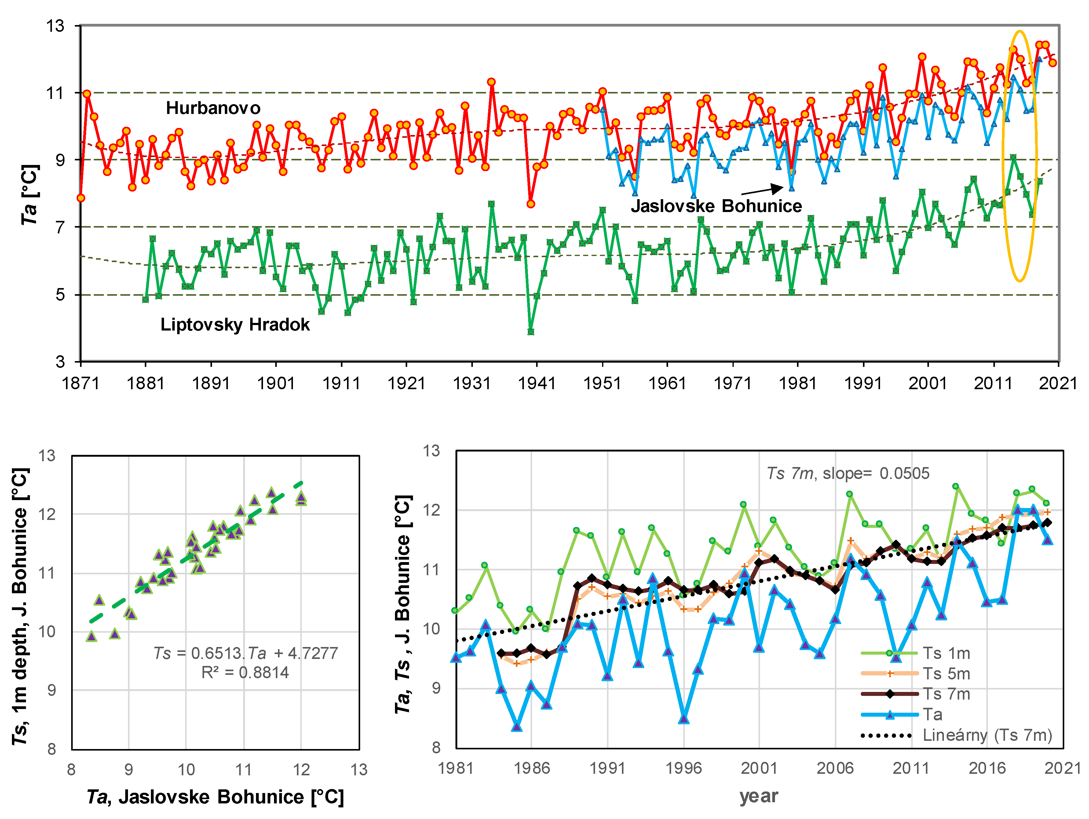
3.1. Long-Term Trends of Air and Soil Temperature Series

In the region of Central Europe, the soil temperature and soil water temperature showed a dependence on the station elevation in a similar way to air temperature and surface water temperature [7]. Therefore, we used air temperature series from stations at different altitudes (Hurbanovo (115 m a.s.l.) and Liptovský Hrádok (640 m a.s.l.)) to illustrate the long-term temperature trends (Figure 4).
These stations had the longest series of air temperature (Ta) observations in Slovakia. Figure 4a presents the annual mean air temperature trends (estimated by a polynomial function of the 5th degree) over the observation period at these two stations. An increase in air temperature was evident, especially after 1989. The soil temperature (Ts) showed a very similar long-term trend. This was evident in the mean annual air temperature series from the Jaslovské Bohunice station (1951–2020, Figure 4a) and the mean annual temperate measured at three depths from the Jaslovské Bohunice meteorological station (1984–2020, Figure 4b). The long-term average temperatures at different depths were higher compared to the air temperature by 0.8 °C at the Jaslovské Bohunice station during the period 1991–2020.

Characteristics of the Soil and Groundwater Temperature Series at Different Stations

A grain size analysis was performed at all the IH SAS stations. The grain size analysis was performed using the densitometric method. Table 2 shows examples of the results from the three stations. At Liptovský Mikuláš, the soil profile was made of sandy loam up to a depth of 1.0 m, which changed to loam at lower depths. The soil profiles at each individual station were relatively homogeneous in terms of vertical grain composition.
There were significant differences in the resulting characteristics of the groundwater temperature series at the different stations (Table 3). The highest mean annual groundwater temperature at its surface over the four-year period 2013–2016 was recorded at Hurbanovo (12.85 °C) in the Danube Lowland, and the lowest was recorded at the Liptovský Mikuláš station (9.65 °C). The highest variation in water temperature at the water table was recorded in Sekule, (7.63–18.17 °C, see Figure 5), and the lowest differences were recorded in the Liptovský Mikuláš station (6.92–12.88 °C). No daily oscillations in temperature were observed below a depth of 60 cm. The long-term mean groundwater temperatures at the surface Tw were higher compared to the air temperature Ta by around 0.8–0.9 °C at all the used stations during the period 2013–2016.

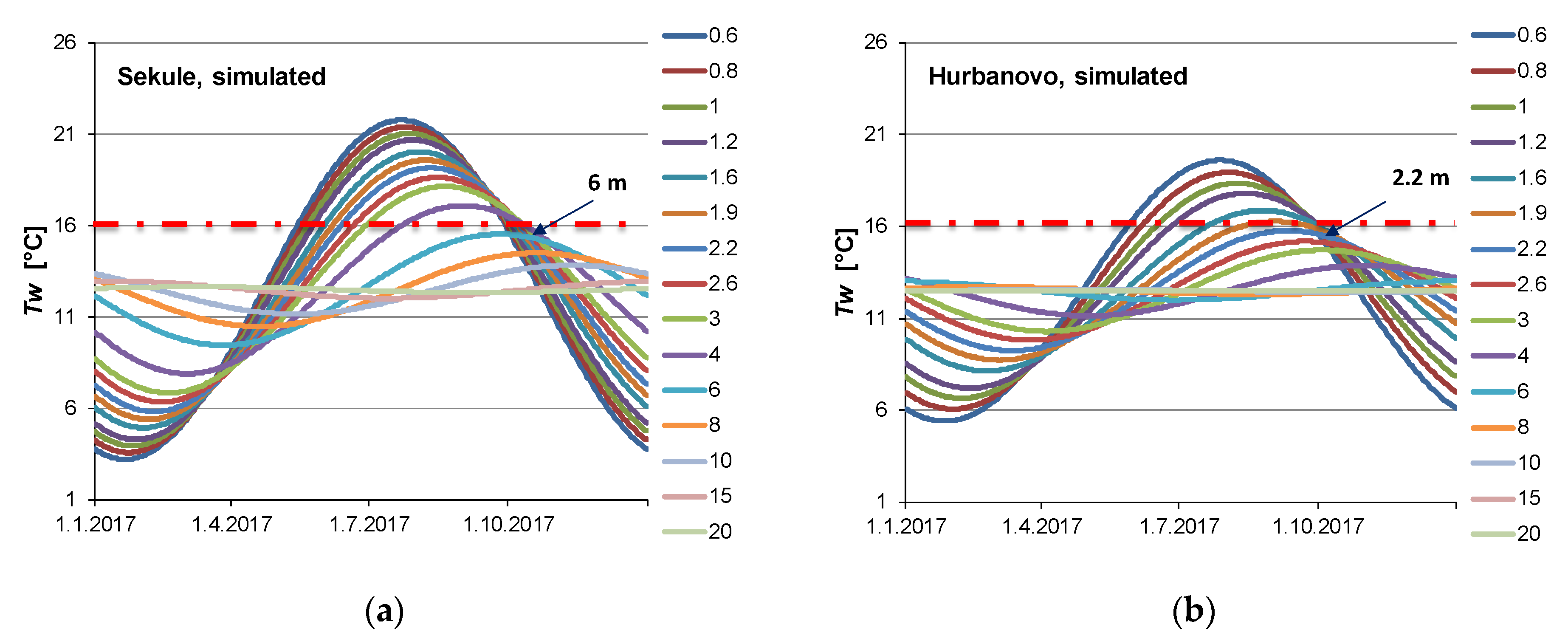
3.2. Results of the Groundwater Temperature Simulation

In this part, the TGWAT model was used based on the modified Equation (3) and air temperature measurements at a given station to simulate the daily soil/ground water temperature at depths greater than 0.6 m. The annual average air temperature minus 0.8 °C was used as the surface (z = 0) annual average temperature of the soil T s ¯ . The three soil parameters (average soil bulk density ρ, soil specific heat capacity C, and soil thermal conductivity k) were estimated from our own measurements and from the literature [31]. Parameters α from equation (4) and ϕ for each station separately were calibrated so that the modelled soil temperatures at 0.8 and 1.6 m depth (Ts,sim) had the highest possible agreement with the measured soil temperatures (Ts,obs). Examples of the calibration results are presented in Figure 6, which shows the modelled (red line) soil temperatures at the four selected stations and the measured soil temperatures (blue line).
The groundwater temperature (Tw) at each station was then simulated with the calibrated TGWAT model at a depth corresponding to the mean annual water table depth. The simulated soil (Ts,sim) water temperature results were compared with the measured temperatures at the groundwater level (Tw,obs) (Figure 7 right). The agreement between measured and simulated temperatures was very good (Figure 7 left), although several simplifications were used. For example, the variation in the groundwater level over the years was not taken into account. From the staircase shape of the water temperature measurements, it can be seen that thermometers with a higher resolution should be used. Table 4 shows the resulting parameters α and ϕ for each station, which were obtained by calibrating the TGWAT model. The temperature of the groundwater in Sekule and Hurbanovo exceeded 16 °C during September–November, so it was not suitable for drinking.
The calibrated model was used to simulate the soil/groundwater temperature to a maximum depth of 20 m. Figure 8 shows the simulated groundwater temperatures at the Sekule and Hurbanovo stations. At the Sekule station at a depth of 6 m, the lowest temperature was in April and the highest was in September. The groundwater temperature was below 16 ° C throughout the year. At a depth of 15 m, the temperature was constant and was 0.8 °C higher than the average annual air temperature at this station. Both stations are located in sedimentary lowlands. Station Sekule is in an area of eolitic sediments and dunes with a depth of 40–80 m. Station Hurbanovo is located in a large fluvial sedimentary basin with sand/gravel layers up to hundreds of meters.

4. Discussion and Conclusions

The analysis of the water temperature measurements showed that the highest mean annual groundwater temperature at the water table during the four-year period 2013–2016 was recorded at Hurbanovo (12.85 °C) in the Danube Lowland, and the lowest was measured at the Liptovský Mikuláš station (9.65 °C). This fact resulted both from the altitude of the stations (Hurbanovo 115 m a.s.l., Liptovský Mikuláš 569 m a.s.l.) and from the location of the stations (south versus north of Slovakia). The highest variation in water temperature at the water table was recorded in Sekule (7.63–18.17 °C) due to its sandy soil. The lowest variations were at the Liptovský Mikuláš station (6.92–12.88 °C) due to its loamy soil.
In the present study, a TGWAT soil/groundwater temperature model for depths greater than 0.6 m was constructed based on the one-dimensional Fourier differential heat conduction equation. The input data required are the average annual air temperature and parameters α and ϕ for the soil type at a given station. In this work, the parameters α and ϕ were specified by calibrating the model based on measurements of the soil temperature at different depths and the groundwater temperature at water table.
The verification of the model showed that the simulated soil temperatures were in good agreement with the measured values of the soil temperature at a depth of up to 1.6 m. To compare the simulated soil temperatures at a depth of 6 m, we plotted the daily soil temperature at four stations and the course of the measured average monthly values of soil temperature at a depth of 6 m at Jaslovské Bohunice and Tisinec stations (Figure 9). The temperature profiles depended on the type of soil, which we did not know at greater depths. Nevertheless, the simulation results were realistic.
The calibrated soil/water temperature model TGWAT has several potential applications. For example, it can be used to complete missing soil and groundwater temperature measurements during measurement failure. The model can be used to estimate the soil temperature at different depths without measurements based on the elevation of the area, the mean annual air temperature, and knowledge of the soil type. Conversely, it is possible to estimate the depth from which the water comes by measuring the temperature of the water in the springs. The given model can also be used to estimate future groundwater temperature trends using regional air temperature projections calculated for different greenhouse gas emission scenarios [31,32,33,34,35,36]. The model TGWAT requires only the mean daily air temperature as the input data. The impact of precipitation [37] on soil temperature is not included explicitly, but it is included indirectly in the air temperature.
The following conclusions can be drawn from the modelled soil water temperatures:
  • From the long-term trend analysis of air temperature and temperatures at depths of up to 10 m, we can see that in Slovakia the air temperature increased by 0.6 and the soil temperature increased by 0.5 °C per 10 years over the past 30 years.
  • The long-term average temperatures at depths up to 10 m were higher compared to the air temperature by around 0.8–0.9 °C at all the used stations during the period 2013–2016.
  • The groundwater temperature at a depth of approximately 6 m in Hurbanovo was highest in the coldest winter months of January–February. This finding should be taken into account when using heat pumps in the construction industry [38] for cooling and heating buildings.
  • Long-term temperature measurements at a depth of approximately 10 m would be useful to verify the atmospheric temperature rise, as this temperature, unlike air temperature measurements, is minimally affected by daily and seasonal variations, by changes in vegetation on the surface, and by the fact that the mass heat capacity of ice is half that of water and a quarter that of air [39].
The presented work brings new knowledge about the development of soil and water temperature in Slovakia at depths of 0.6–10 m. The acquired knowledge has a very wide application potential in the assessment of water temperature development and climate change assessment.

Supplementary Materials

The following supporting information can be downloaded at: www.mdpi.com/article/10.3390/hydrology9100185/s1, Figure S1: Location of the 35 probes throughout Slovakia equipped with data teletransmission (2012–2020); Table S1: Location and land use of measuring sites where automatic measuring probes were installed.

Author Contributions

Conceptualization, P.P. and P.M.; methodology, P.P.; original draft preparation; P.P., writing, P.P. and J.P.; software, J.P.; formal analysis, J.P., J.V. and P.M.; visualization, P.P. and A.T.; review and editing, P.M.; data curation, A.T. and J.V. All authors have read and agreed to the published version of the manuscript.

Funding

This research was funded by the project APVV-20-0374 “Regional detection, attribution and projection of impacts of climate variability and climate change on runoff regimes in Slovakia”, project WATSIM “Water temperature simulation during summer low flow conditions in the Danube basin”, and the grants VEGA No. 2/0044/20 “Quantification of interaction processes in hydrological cycle in lowland area conditions” and VEGA No. 2/0004/19 “Analysis of changes in surface water balance and harmonization of design discharge calculations for estimation of flood and drought risks in the Carpathian region”.

Data Availability Statement

Not applicable.

Acknowledgments

This study resulted from the project implementation “Centre of excellence for the integrated river basin management in the changing environmental conditions” (ITMS code 26220120062) and “Infrastructure completion of hydrological research stations” (ITMS code 2621012009), supported by the Research & Development Operational Programme funded by the ERDF. http://www.uh.sav.sk/en-gb/Research/Centre-of-Excellence (accessed on 22 August 2022). The authors would like to thank all colleagues who participated in the establishing and operation of the station network.

Conflicts of Interest

The authors declare no conflict of interest.

References

  1. Davidson, E.A.; Janssens, I.A. Temperature sensitivity of soil carbon decomposition and feedbacks to climate change. Nature 2006, 440, 165–173. [Google Scholar] [CrossRef] [PubMed] [Green Version]
  2. Riedel, T. Temperature-associated changes in groundwater quality. J. Hydrol. 2019, 572, 206–212. [Google Scholar] [CrossRef]
  3. Miklánek, P.; Martincová, M.; Pekárová, P.; Mészároš, I. Seasonal changes of the soil temperature in different depths. In Proceedings of the 13th International Multidisciplinary Scientific GeoConference SGEM 2013: Hydrology and Water Resources, Soil, Forest Ecosystems, Marine and Ocean Ecosystems, Sofia, Bulgaria, 16–22 June 2013; pp. 285–292. [Google Scholar]
  4. Dunajsky, E. Soil Temperature in Greater Depths, Slovakia. Available online: http://www.shmu.sk/File/sms/dunajsky_teplota.pdf (accessed on 1 September 2022). (In Slovak).
  5. Limberg, A.; Henning, A. Auswertung von Temperaturmessungen des Berliner Untergrundes über einen Zeitraum von 150 Jahren. Brandenbg. Geowiss. Beitr. 2019, 26, 15–31. [Google Scholar]
  6. Marcin, D.; Benková, K.; Fričovský, B.; Bodiš, D.; Bottlik, F.; Kordík, J.; Stríček, I. Assessment of the State of Geothermal Bodies of Ground Water in the Territory of the Slovak Republic; Geological study; State Geological Institute of Dionýz Štúr: Bratislava, Slovak, 2020; p. 295, 22 appendixes. [Google Scholar]
  7. Martincová, M.; Pekárová, P.; Škoda, P.; Pekár, J. Long-term trends in water temperature in the Slovak rivers and the impact of climatic and orographic factors. Acta Hydrol. Slovaca. 2011, 12, 276–285. [Google Scholar]
  8. Bedrna, Z.; Gašparovič, J. Types of temperature regime of the soils in the Czechoslovak socialist republic. Geogr. Časopis. 1986, 38, 60–77. (In Slovak) [Google Scholar]
  9. Song, Y.T.; Zhou, D.W.; Zhang, H.X.; Li, G.D.; Jin, Y.H.; Li, Q. Effects of vegetation height and density on soil temperature variations. Chin. Sci. Bull. 2013, 58, 907–912. [Google Scholar] [CrossRef] [Green Version]
  10. Nikiforova, T.; Savytskyi, M.; Limam, K.; Bosschaerts, W.; Belarbi, R. Methods and results of experimental researches of thermal conductivity of soils. Energy Procedia. 2013, 42, 775–783. [Google Scholar] [CrossRef] [Green Version]
  11. Kodešová, R.; Vlasáková, M.; Fér, M.; Teplá, D.; Jakšík, O.; Neuberger, P.; Adamovský, R. Thermal properties of representative soils of the Czech Republic. Soil Water Res. 2013, 8, 141–150. [Google Scholar] [CrossRef] [Green Version]
  12. Özkan, U.; Gökbulak, F. Effect of vegetation change from forest to herbaceous vegetation cover on soil moisture and temperature regimes and soil water chemistry. Catena 2017, 149, 158–166. [Google Scholar] [CrossRef]
  13. Šimůnek, J.; Šejna, M.; Saito, H.; van Genuchten, M.T. The HYDRUS-1D Software Package for Simulating the One-Dimensional Movement of Water, Heat, and Multiple Solutes in Variably-Saturated Media; Department of Environmental Science, University of California Riverside: Riverside, CA, USA, 2013. [Google Scholar]
  14. Valuš, G. Soil temperatures. In Climatic and Phenological Conditions of the East Slovak Region, 1st ed.; HMI: Prague, Czech Republic, 1966; pp. 118–123. [Google Scholar]
  15. Coufal, V.; Kott, I.; Moãný, M. Soil temperature in the cold part of the year in the period 1961–1991 in the Czech Republic. In National Climate Program of the Czech Republic; Czech Hydrometeorological Institute: Prague, Czech Republic, 1993; p. 37. (In Czech) [Google Scholar]
  16. Hora, P. Relationship between soil temperature and different soil types. In Mikroklima a Mezoklima Krajinných Struktur a Antropogenních Prostředí; Středová, H., Rožnovský, J., Litschmann, T., Eds.; CHMI: Praha, Czech Republic, 2011. [Google Scholar]
  17. Kutílek, M. Hypothermic soil regimes. In Pedologie a Paleo-Pedologie; Němeček, J., Smolíková, L., Kutílek, M., Eds.; Academia: Praha, Czech Republic, 1990; pp. 86–99. (In Czech) [Google Scholar]
  18. Kočárek, M.; Kodešová, R. Influence of temperature on soil water content measured by ECH2O-TE sensors. Int. Agrophys. 2012, 26, 259–269. [Google Scholar] [CrossRef]
  19. Lehnert, M. The soil temperature regime in the urban and suburban landscapes of Olomouc, Czech Republic. Morav. Geogr. Rep. 2013, 21, 3, 27–36. [Google Scholar] [CrossRef] [Green Version]
  20. Zheng, D.; Hunt, E.R., Jr.; Running, S.W. A daily soil temperature model based on air temperature and precipitation for continental applications. Clim. Res. 1993, 2, 183–191. [Google Scholar] [CrossRef]
  21. Taylor, C.A.; Stefan, H.G. Shallow groundwater temperature response to climate change and urbanization. J. Hydrol. 2009, 375, 601–612. [Google Scholar] [CrossRef]
  22. Riedel, J.W.; Peterson, E.W.; Dogwiler, T.J.; Seyoum, W.M. Investigating thermal controls on the hyporheic flux as evaluated using numerical modeling of flume-derived data. Hydrology 2022, 9, 156. [Google Scholar] [CrossRef]
  23. Kassaye, K.T.; Boulange, J.; Tu, L.; Saito, H.; Watanabe, H. Soil water content and soil temperature modeling in a vadose zone of Andosol under temperate monsoon climate. Geoderma 2021, 384, 114797. [Google Scholar] [CrossRef]
  24. Singh, R.K.; Sharma, R.V. Numerical analysis for ground temperature variation. Geotherm Energy 2017, 5, 22. [Google Scholar] [CrossRef] [Green Version]
  25. Wang, J.; Lee, W.F.; Ling, P.P. Estimation of Thermal Diffusivity for Greenhouse Soil Temperature Simulation. Appl. Sci. 2020, 10, 653. [Google Scholar] [CrossRef] [Green Version]
  26. Park, K.; Kim, Y.; Lee, K.; Kim, D. Development of a Shallow-Depth Soil Temperature Estimation Model Based on Air Temperatures and Soil Water Contents in a Permafrost Area. Appl. Sci. 2020, 10, 1058. [Google Scholar] [CrossRef] [Green Version]
  27. Sándor, R.; Fodor, N. Simulation of soil temperature dynamics with models using different concepts. Sci. World J. 2012, 8, 590287. [Google Scholar] [CrossRef] [PubMed] [Green Version]
  28. Wang, L.; Gao, Z.; Horton, R.; Lenschow, D.H.; Meng, K.; Jaynes, D.B. An analytical solution to the one-dimensional heat conduction–convection equation in soil. Soil Sci. Soc. Am. J. 2012, 76, 1978–1986. [Google Scholar] [CrossRef] [Green Version]
  29. Islam, M.A.; Lubbad, R.; Amiri, S.A.G.; Isaev, V.; Shevchuk, Y.; Uvarova, A.V.; Afzal, M.S.; Kumar, A. Modelling the seasonal variations of soil temperatures in the Arctic coasts. Polar Sci. 2021, 30, 100732. [Google Scholar] [CrossRef]
  30. Andújar Márquez, J.M.; Martínez Bohórquez, M.Á.; Gómez Melgar, S. Ground thermal diffusivity calculation by direct soil temperature measurement. Application to very low enthalpy geothermal energy systems. Sensors 2016, 16, 306. [Google Scholar] [CrossRef] [PubMed] [Green Version]
  31. Farouki, O.T. Thermal Properties of Soils. Ser. Rock Soil Mech. 1986, 11, 136. [Google Scholar]
  32. Peters-Lidard, C.D.; Blackburn, E.; Liang, X.; Wood, E.F. The Effect of Soil Thermal Conductivity Parameterization on Surface Energy Fluxes and Temperatures. J. Atmos. Sci. 1998, 55, 1209–1223. [Google Scholar] [CrossRef]
  33. Kodešová, R.; Fér, M.; Klement, A.; Nikodem, A.; Teplá, D.; Neuberger, P.; Bureš, P. Impact of various surface covers on water and thermal regime of Technosol. J. Hydrol. 2014, 519, 2272–2288. [Google Scholar] [CrossRef]
  34. Figura, S.; Livingstone, D.M.; Kipfer, R. Forecasting groundwater temperature with linear regression models using historical data. Groundwater 2015, 53, 943–954. [Google Scholar] [CrossRef]
  35. Riedel, T.; Weber, T.K.D. Review: The influence of global change on Europe’s water cycle and groundwater recharge. Hydrogeol J. 2020, 28, 1939–1959. [Google Scholar] [CrossRef]
  36. Michel, A.; Schaefli, B.; Wever, N.; Zekollari, H.; Lehning, M.; and Huwald, H. Future water temperature of rivers in Switzerland under climate change investigated with physics-based models. Hydrol. Earth Syst. Sci. 2022, 26, 1063–1087. [Google Scholar] [CrossRef]
  37. Lei, N.; Han, J. Effect of precipitation on respiration of different reconstructed soils. Sci. Rep. 2020, 10, 7328. [Google Scholar] [CrossRef]
  38. Leski, K.; Luty, P.; Gwadera, M.; Larwa, B. Numerical Analysis of Minimum Ground Temperature for Heat Extraction in Horizontal Ground Heat Exchangers. Energies 2021, 14, 5487. [Google Scholar] [CrossRef]
  39. Pekárová, P.; Pekár, J.; Miklánek, P. Why do some places show a bimodal distribution of daily air temperature? In Water Regime of Natural Areas: Book of Peer-Reviewed Papers; IH SAS: Bratislava, Slovakia, 2022; pp. 20–29. ISBN 978-80-89139-52-1. (In Slovak) [Google Scholar]
Figure 1. (a) Long-term monthly observed temperature (Ts) at different depths and the development of long-term temperature in individual months at different depths (z) at Jaslovské Bohunice meteorological station, 1991–2020. (b) Scheme of the air thermal gradient and geothermal gradient, Jaslovské Bohunice.
Hydrology 09 00185 g001
Figure 2. (a) Scheme of Slovakia (49,000 km2)—the position of four selected IH SAS stations (blue points), position of the lysimetric station (Petrovce nad Laborcom (red point)), and stations for measuring temperature at great depths up to 10 m at Tisinec and Jasovské Bohunice (black points). (b) Location of the 35 probes throughout Slovakia equipped with data teletransmission (2012–2020). See Supplementary Materials.
Hydrology 09 00185 g002
Figure 3. Measured soil temperatures at 22 depths at the lysimeter station in Petrovce n. Laborcom in 2015 at hourly intervals.
Hydrology 09 00185 g003
Figure 4. Mean annual air temperature (Ta) at the Hurbanovo (1871–2020), Liptovský Hrádok (1881–2018), and Jaslovské Bohunice (1951–2018) stations with polynomial long-term trends (dashed lines). Relationship between the Ta at Jaslovské Bohunice and Ts at 1 m depth at Jaslovské Bohunice (bottom left). Mean annual air temperature at Jaslovské Bohunice (1981–2020) and mean annual temperatures at 1 m, 5 m, and 7 m depth at Jaslovské Bohunice meteorological station (1984–2020) with the linear long-term trend +0.05 °C per year (bottom right).
Hydrology 09 00185 g004
Figure 5. Daily measured soil Ts, groundwater temperature Tw, and depth of the groundwater table at the Sekule station during the period 2013–2016 (data measured at 7 a.m.).
Hydrology 09 00185 g005
Figure 6. Daily modelled (Ts,sim) and measured (Ts,obs) soil temperatures at depths of 0.8 and 1.6 m over the period 2013–2014 (the calibration period). Stations: 1. Sekule, 2. Hurbanovo, 3. Streda n. Bodrogom, and 4. Liptovský Mikuláš.
Hydrology 09 00185 g006
Figure 7. Simulated (Ts,sim) and measured groundwater temperatures (Tw,obs) at the mean depth of the groundwater level over the period 2013–2016 (left); relation between measured and modelled values (right).
Hydrology 09 00185 g007
Figure 8. Simulated soil/groundwater temperatures at depths of 0.6–20 m at stations (a) Sekule and (b) Hurbanovo in 2017. Minimum depth where the groundwater temperature was less than 16 °C throughout the year at Sekule was 6 m, and at Hurbanovo it was 2.2 m.
Hydrology 09 00185 g008
Figure 9. Comparison of the daily simulated soil temperatures (Tsim) at a 6 m depth at four stations (top) and the measured average monthly soil temperature (Tm) at a 6 m depth at the Jaslovské Bohunice and Tisinec stations (bottom) over the period 2014–2015.
Hydrology 09 00185 g009
Table 1. Location, land use, and type of soil of measuring sites where automatic measuring probes were installed.
No.LocalityLand UseType of SoilGPS
NE
01VinnéVineyard, grassClay loam48°48.842′21°57.812′
02BracovceOrchard, grass Clay loam48°38.584′21°50.094′
03Pavlovce Orchard, grass Clay loam48°36.702′22°04.170′
04LastomírOrchard, grass Sandy loam48°42.230′21°55.631′
05StrážskeOrchard, grass Clay loam48°52.069′21°49.836′
06SekuleOrchard, grassLoamy sand48°36.383′16°59.675′
07Hurbanovo 1Orchard, grassLoamy sand47°53.055′18°10.298′
08Nitra 1LawnClay loam48°18.150′18°05.980′
09IňačovcePastureland, grassSilty-clay loam48°41.304′22°03.198′
10Streda n. BodrogomAgricultural cropsClay loam48°21.526′21°44.659′
11PoľanyPastureland, grassSandy loam 48°27.997′21°59.044′
12BoľPastureland, grassClay loam48°28.495′21°56.774′
13Liptovský MikulášLawnLoam49°05.838′19°35.392′
14JastrabieAgricultural cropsClay loam48°43.199′22°01.727′
15KoňušVineyard, grassClay loam48°46.383′22°15.639′
16PinkovceOrchard, grassClay loam48°36.325′22°11.056′
17Zemplínska ŠirokáOrchard, grasslay loam48°42.007′21°58.192′
18Nitra 3Orchard, grassClay loam48°18.082′18°06.117′
19Nitra 2Orchard, grassClay loam48°18.121′18°06.054′
20Hurbanovo 2LawnLoam47°52.345′18°11.573′
21Nitra 4Orchard, grassClay loam48°18.010′18°05.971′
22Nitra 5Orchard, grassClay loam48° 18.208′18° 05.791′
23VrakúňAgricultural cropsLoamy sand47°56.428′17°37.025′
24TopoľníkyOrchard, grassLoam47° 58.593′17° 46.623′
25KamenínVineyard, grassLoam47°53.315′18°38.463′
26Vydrany 1Agricultural cropsLoam48°01.988′17°35.907′
27Vydrany 2Agricultural cropsLoam48°03.884′17°39.005′
28SalkaAgricultural cropsLoamy sand47°53.918′18°44.795′
29NánaAgricultural cropsLoam47°49.010′18°41.593′
30Kamenný MostOrchard, grassSandy loam47°51.130′18°39.218′
Table 2. Examples of grain size analysis at the Sekule, Hurbanovo, and Streda above Bodrog IH SAS stations.
DepthMean Particle DensityBulk
Density
Soil Texture
ρsρbClaySiltSandTextural Class
<0.002 mm0.002–0.05 mm0.05–2.00 mm
[cm][g·cm−3][g·cm−3][%][%][%]
Sekule (48°36.383′ N, 16°59.675′ E)
102.581.4610.815.0984.10Loamy sand
202.631.537.8910.3181.80Loamy sand
402.601.7110.526.0883.40Loamy sand
602.581.7810.610.9988.40Loamy sand
802.611.7710.620.4888.90Loamy sand
1002.731.7010.420.0889.50Loamy sand
1202.631.8410.520.1889.30Loamy sand
1602.661.7010.620.0889.30Loamy sand
Hurbanovo (47°52.345′ N, 18°11.573′ E)
102.591.1013.5433.7652.70Sandy loam
202.651.2114.9130.0955.00Sandy loam
402.691.727.6227.0865.30Sandy loam
602.661.2315.7728.2356.00Sandy loam
802.691.3916.9325.8757.20Sandy loam
1002.691.4815.5228.0856.40Sandy loam
1202.691.5312.8619.3467.80Sandy loam
1602.701.4619.5724.7355.70Sandy loam
Streda nad Bodrogom (48°21.526′ N, 21°44.659′ E)
102.661.4123.0157.6919.30Silt loam
202.651.4924.6956.9118.40Silt loam
402.641.3822.9351.4725.60Silt loam
602.681.3523.1654.1422.70Silt loam
802.751.3120.1255.2824.60Silt loam
1002.771.3120.7060.8018.50Silt loam
1202.671.2115.1843.5241.30Loam
1602.691.4335.1655.649.20Silty clay loam
Table 3. Baseline characteristics of groundwater temperature (Tw) at four selected stations for the period 1.1.2013–31.12.2016.
SekuleHurbanovoStreda n. BodrogomL. Mikuláš
Groundwater level [m]31.92.43
Tw mean [°C]12.8012.8511.809.65
Tw min [°C]7.639.569.086.92
Tw max [°C]18.1717.2414.9212.88
Tw stdev [°C]3.732.712.072.11
Ta mean [°C]11.9911.7111.008.27
Table 4. Parameters α and ϕ for selected stations (results of the TGWAT model calibration) over the period 1.1.2013–31.12.2016.
SekuleHurbanovoStreda n BodrogomL. Mikuláš
Soil textural classloamy sandsandy loamsilt loamloam
α [m2.day−1]0.16520.03640.03180.0533
ϕ [rad]0.250.180.200.24
Groundwater level [m]3.41.742.433
Tw average [°C]12.9012.8511.809.65
Ta average [°C]11.9911.7111.008.27
Publisher’s Note: MDPI stays neutral with regard to jurisdictional claims in published maps and institutional affiliations.

