Analysis of Groundwater Depletion in the Saskatchewan River Basin in Canada from Coupled SWAT-MODFLOW and Satellite Gravimetry

Abstract

The Saskatchewan River Basin (SRB) of central Canada plays a crucial role in the Canadian Prairies. Yet, climate change and human action constitute a real threat to its hydrological processes. This study aims to evaluate and analyze groundwater spatial and temporal dynamics in the SRB. Groundwater information was derived and compared using two different approaches: (1) a mathematical modeling framework coupling the Soil and Water Assessment Tool (SWAT) and the Modular hydrologic model (MODFLOW) and (2) gravimetric satellite observations from the Gravity Recovery and Climate Experiment (GRACE) mission and its follow-on (GRACE-FO). Both methods show generalized groundwater depletion in the SRB that can reach −1 m during the study period (2002–2019). Maximum depletion appeared especially after 2011. The water balance simulated by SWAT-MODFLOW showed that SRB could be compartmented roughly into three main zones. The mountainous area in the extreme west of the basin is the first zone, which is the most dynamic zone in terms of recharge, reaching +0.5 m. The second zone is the central area, where agricultural and industrial activities predominate, as well as potable water supplies. This zone is the least rechargeable and most intensively exploited area, with depletion ranging from +0.2 to −0.4 m during the 2002 to 2011 period and up to −1 m from 2011 to 2019. Finally, the third zone is the northern area that is dominated by boreal forest. Here, exploitation is average, but the soil does not demonstrate significant storage power. Briefly, the main contribution of this research is the quantification of groundwater depletion in the large basin of the SRB using two different methods: process-oriented and satellite-oriented methods. The next step of this research work will focus on the development of artificial intelligence approaches to estimate groundwater depletion from a combination of GRACE/GRACE-FO and a set of multisource remote sensing data.

1. Introduction

Climate change could spatially and temporally affect several crucial components of the hydrological cycle, including precipitation, evapotranspiration, soil temperature and water content, and surface runoff, together with river flow [1,2,3]. These changes in hydrological conditions, in turn, could lead to multiple effects on groundwater and subsurface flows, as has been reported in various studies [4,5]. In particular, aquifer recharge and discharge rates could be greatly altered [6,7], together with disrupting water flow and storage [8,9]. These disturbing issues, when combined with higher water demands that are generated by human activities in many regions, call for a better understanding of the processes and accurate estimation of various hydrological components of the water cycle for decision-making with respect to resource planning and management by governments [10]. Such improvements are particularly crucial for arid and semi-arid areas in the world, which are characterized by water scarcity and frequent droughts.

To allow for better understanding and management, scientists have developed several tools for conceptualizing and modelling water resource flows and stocks. These tools are mainly process-oriented and are essentially based on the construction of coupled hydrological models, the understanding and conceptualization of complex systems, and the quantification of the various transfers between the atmosphere, snow cover, soil, and vegetation. Coupled hydrogeological modelling is being increasingly used for analyzing complex hydrological systems in the context of climate change [11,12]. SWAT-MODFLOW is one of the most widely used coupled hydrogeological models. SWAT (Soil Water Assessment Tool) is a watershed-scale semi-distributed model that can simulate surface flow and runoff. It has been demonstrated to perform well in simulating stream flows in a wide range of watersheds and has been tested in many regions, conditions, and time scales [13,14]. The most frequently used approach to improving the performance of SWAT in watersheds that encompass developed aquifer systems is to couple the former with a physics-based, spatially distributed numerical groundwater model, such as MODFLOW (Modular Finite-Difference Flow Model). MODFLOW was developed by the United States Geological Survey (USGS) and has been continually refined since it debuted in the 1980s (current release: MODFLOW 6.2.2). It is a multilayer finite-difference model that is used to model aquifer systems and complex groundwater flow problems [15]. MODFLOW has been tested and used in various practical cases [16,17]. The coupled SWAT-MODFLOW system has been adapted to and implemented in several study areas around the world [18,19,20].

A common difficulty that emerges from using such complex modelling systems is related to the availability of reliable observation data that are capable of characterizing the complexities of watersheds and aquifers. Data could come from field surveys or continuous observations through stations. The main disadvantage is that measurements are often discrete and periodic in time and space; therefore, interpolation is required to estimate the input variables over the entire basins being studied. Furthermore, installation and monitoring of continuous measurement devices could be costly and, thus, are most frequently limited to densely populated areas.

In this context, the use of remotely sensed data appears as an alternative complementary solution that would fulfill the need for information regarding several relevant hydrological variables. For instance, land cover data that are extracted from remote sensing, together with vegetation indices or soil moisture, are used in many hydrological studies. For hydrogeology and groundwater stock characterizations, gravimetric satellite data figures are among the most relevant observations to be considered. The Gravity Recovery and Climate Experiment (GRACE) mission provided total water storage (TWS) measurements from 2002 to 2017 (https://www2.csr.utexas.edu/grace/) (accessed on 10 august 2023). Its follow-on (GRACE-FO) has been pursuing the mission since 2018. TWS represents the total water column from snow to groundwater, making it relevant information that is uniquely suited to continental hydrology investigations. Several studies [21,22,23,24] have shown that the accuracy of TWS estimates is within several millimeters and that the hydrological signal is likely influenced by noise that is caused by short wavelengths. Despite the very coarse spatial and temporal resolution of GRACE and GRACE-FO data, their level of accuracy makes them particularly relevant to large-scale hydrology. Yet, investigations are still required to improve the accuracy and spatial and temporal resolution of these data so that they may be exploited to their full potential [24,25]. For instance, groundwater information that is extracted from satellite gravimetry could provide a comparable basis for the simulation results of process-based models, such as the coupled SWAT-MODFLOW.

Combined use of coupled modelling and GRACE and GRACE-FO observations could contribute to a better understanding of complex hydrogeologic systems under changing climate conditions in arid and semi-arid areas that are facing ongoing water shortages or flood problems. The Saskatchewan River Basin (SRB), which is located in the Canadian Prairies, is such an area that is characterized by intense and high-frequency drought events, a decrease in river flow, and a generalized depletion of the aquifer system. According to the Canadian Drought Monitor (CDM) of Agriculture and Agri-Food Canada, which is the official Canadian source for reporting drought events, the Canadian Prairies region is considered a “hot spot” for drought events and their impacts on water resources. In the Canadian context, SRB is potentially the basin that is most vulnerable to global change. Groundwater resources in the basin remain a highly uncertain component, despite their wide use in southern regions for human activities [26]. Moreover, studies regarding the effects of drought on the availability of this resource are scarce. Decision makers in this basin are still looking for greater knowledge that would better guide the management of water resources in the changing environmental conditions.

The main motivation of this study arises from the need for advanced knowledge on the hydrogeology and water resources of the SRB, a basin where data are scarce and fragmentary. The main objective of the research is to evaluate the potential of remote sensing and hydrogeological modelling for monitoring and understanding the response of a complex aquifer system to climate change and anthropogenic stress (drought and over-exploitation). The specific objectives in the paper are (i) the implementation of a Coupled SWAT-MODFLOW to estimate groundwater storage variation in the SRB; (ii) the use of GRACE/GRACE-FO data to estimate groundwater storage and trend variations; (iii) to estimate and compare the process-oriented (SWAT-MODFLOW) and satellite-based method (GRACE/GRACE-FO) for groundwater potential depletion.

2. Study Area

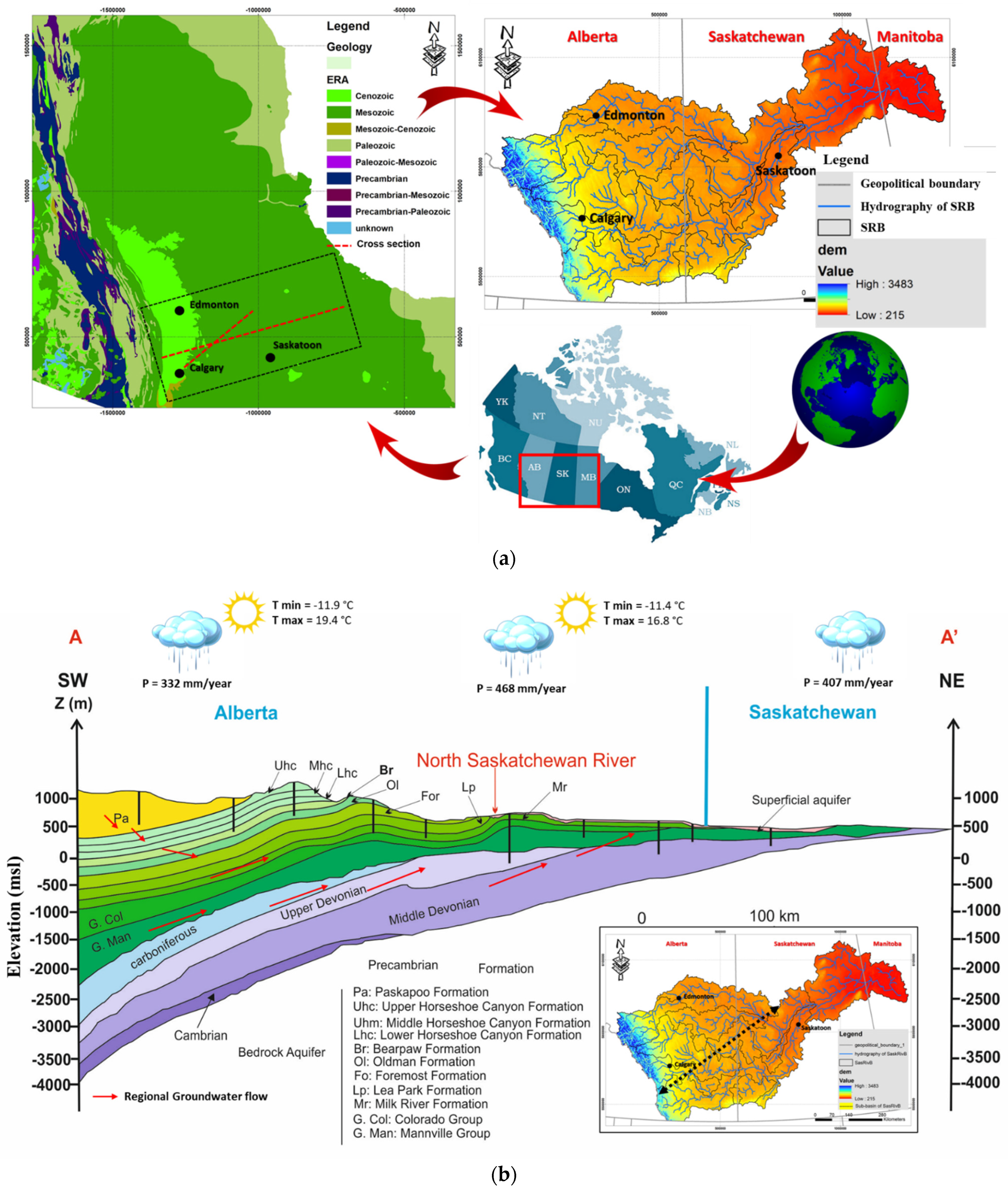
The Canadian Prairies region is located in the central part of Canada, encompassing the provinces of Alberta (AB), Saskatchewan (SK), and Manitoba (MB) (Figure 1). This region is known for its vast grasslands, fertile farmlands, and rolling hills. It is an important agricultural and energy-producing region, with a diverse economy that includes farming in the southern part, oil and gas extraction, and manufacturing. The climate is characterized by long cold winters and short warm summers, which are favourable for growing annual crops (wheat, barley, and canola, among others). Groundwater exploitation in the Canadian Prairies has been a concern for many decades. The region has experienced substantial population growth and industrialization, which has led to increased demand for water resources. Groundwater is a critical resource for several usages (drinking water, irrigation, and industrial purposes). The high pressure imposed on groundwater exploitation has led to several negative impacts, including declining water levels and quality, as well as increased pumping costs. Over-pumping of groundwater can cause aquifer depletion and eventually jeopardize the long-term sustainability of water resources. In addition, groundwater could also be contaminated by human activities, such as agricultural runoff, with serious implications for the environment and public health. Further information regarding water resources in the Canadian Prairies can be found in [27].

The geological map of the SRB (Figure 1) shows extensive Upper Cretaceous outcrops. These outcrops extend across the entire interior shelf area. The lower Cretaceous series extends along the edges of the basin forming a halo. The Upper Cretaceous includes a series that is formed mainly by deposits of sands, shales, coals, and clays. The most recent series outcrop in the southwestern part of the basin. These Upper Cretaceous series are of Campanian age (83.6–72 Ma BP) and are spatially discontinuous. They also include the Palaeocene (66–56 Ma), Miocene (23–5 Ma), and Quaternary series (2.6 Ma to present) of the Cenozoic Era. The reader interested in these geological aspects will find more information in [28,29].

On a regional scale, the Saskatchewan Basin (SRB) is situated within the broader geological context of the Interior Platform domain. Within this domain, the predominant rock formations are of Cretaceous age. Specifically, the outcropping series in this region are primarily from the Cretaceous period. It is worth noting that in some areas, these Cretaceous series are covered by more recent Quaternary deposits. The natural boundaries of the basin are defined by various structural features and geometries. To the southwest, the basin is limited by the Cordilleran Orogeny, which gave rise to the formation of the Rocky Mountains. This mountainous region is characterized by large-scale faults, folded geological structures, and a thrust zone. On the northeast side of the Interior Platform domain, the basin is delimited by the Bear, Slave, and Churchill regions. These areas exhibit distinct folding patterns and basin zones, often bounded by normal faults. The eastern boundary of the basin is marked by volcanic zones, signifying the presence of volcanic activity in that region. A glance at the stratigraphic column for the Saskatchewan Basin, as depicted in Figure 1, reveals extensive outcrops of Upper Cretaceous formations. These Upper Cretaceous formations are widespread throughout the Interior Platform domain. In addition to the Upper Cretaceous rocks, the Lower Cretaceous series extends to the edges of the basin, creating a surrounding halo-like pattern. The Upper Cretaceous series in the Saskatchewan Basin predominantly consists of deposits such as sands, shales, coal, and clays. Notably, the Upper Cretaceous series are primarily of Campanian age. These formations are spatially discontinuous and incorporate deposits from the Paleocene, Miocene, and Quaternary periods. This rich geological history contributes to the complex stratigraphy of the region.

3. Long-Term In-Situ and Remote Sensing Data

To achieve better characterization of aquifers and their responses to climate change, it is essential to collect the maximum quantity of information that is available, process it and verify its homogeneity so that modelling of flows could be as realistic as possible. Before interpreting the hydrogeological data, preliminary verification steps are essential, given that they often originate from different sources (different provinces), and their acquisition protocol is harmonized neither in space nor in time. Points within the monitoring network can vary from one campaign to another, and the dates of these campaigns are not necessarily controlled; greater attention is focused on the periods (high water level and low water level periods) than on the dates themselves. In this study, we collected and archived all available hydrogeological data from different agencies and government sites. The data that were collected are summarized in

Table 1. Summary of hydrogeological and remote sensing data that were collected.

Category	Data Type	Description	Sources
Climate	Precipitation + Temperature + Wind + Humidity relative + Sunshine	Daily measurements (2002–2019)	Source: The POWER Project, supported by NASA Earth Science’s Applied Sciences Program https://power.larc.nasa.gov/
Hydrology–Hydrogeology	Hydraulic wells	Structure, Lithology, Hydrodynamic parameters	Source 1 (Alberta): Alberta Water Well Information Database https://www.alberta.ca/alberta-water-well-information-database.aspx
		Pump tests conducted on public and private water wells	Source 2 (Saskatchewan): Water Security Agency, Saskatchewan https://www.wsask.ca/water-info/ground-water/observation-well-network/
	Piezometry	Piezometric histories for several monitoring points	Source 1 (Alberta): Groundwater Observation Well Network, Alberta https://www.alberta.ca/lookup/groundwater-observation-well-network.aspx
			Source 2 (Saskatchewan): Water Security Agency, Saskatchewan https://www.wsask.ca/water-info/ground-water/observation-well-network/
	Surface water	Gauging in control sections: water level, daily, monthly, and annual flow, and their characteristics (Conductance, Topography, among others)	Environment and Climate Change Canada Data Explorer, HYDAT database, https://www.canada.ca/fr/environnement-changement-climatique/services/eau-apercu/volume/surveillance/releves/produits-donnees-services/archives-nationales-hydat.html
	Soil data	SWAT-Food and Agriculture Organization (FAO) database	https://www.fao.org/land-water/land/land-governance/land-resources-planning-toolbox/category/details/en/c/1111246/
	GLDAS (Global Land Data Assimilation System)	Soil moisture, canopy water and snow-water equivalent	https://ldas.gsfc.nasa.gov/gldas
Geology	Stratigraphy and tectonics	1:250,000 geological maps that have been digitized	GEOSCAN (Geological Survey of Canada [GSC] Publications Database, https://geoscan.nrcan.gc.ca/starweb/geoscan/servlet.starweb?path=geoscan/geoscan_f.web
Gas and Oil Wells	Header	Licensee, status, fluid (water or gas), type (exploitation or injection), depths, location,	Petro Ninja Maps, https://petroninja.com/
	Drill/Summary	Casing, cements, completion summary
	Geology of the well	Stratigraphic log: depths and formation
Remote Sensing Data	Gravimetric data GRACE/GRACE-FO	GRACE data (Gravity Recovery and Climate Experiment)	https://grace.jpl.nasa.gov/data/get-data/
	Modis	Net Evapotranspiration 8-Day L4 Global 500 m (Mod16a2)	https://lpdaac.usgs.gov/products/myd16a2v006/
	Earth data	NASA Shuttle Radar Topography Mission (SRTM)	https://earthdata.nasa.gov/nasa-shuttle-radar-topography-mission-srtm-version-3-0-global-1-arc-second-data-released-over-asia-and-australia
	TRMM	The Tropical Rainfall Measuring Mission	https://disc.gsfc.nasa.gov/
	NARR	North American Regional Reanalysis	https://www.ncei.noaa.gov/products/weather-climate-models/north-american-regional
	Land Cover	ESA. Land Cover CCI Product User Guide Version 2.	http://maps.elie.ucl.ac.be/CCI/viewer/download/ESACCI-LC-Ph2-PUGv2_2.0.pdf

Note: All web links for data access were tested at the date of the submission of the paper (10 August 2023).

. The hydrogeological data in question are of two different origins: archival hydrogeological data and remote sensing data. In the second step, we verified, checked, and harmonized the data.

4. Methodology

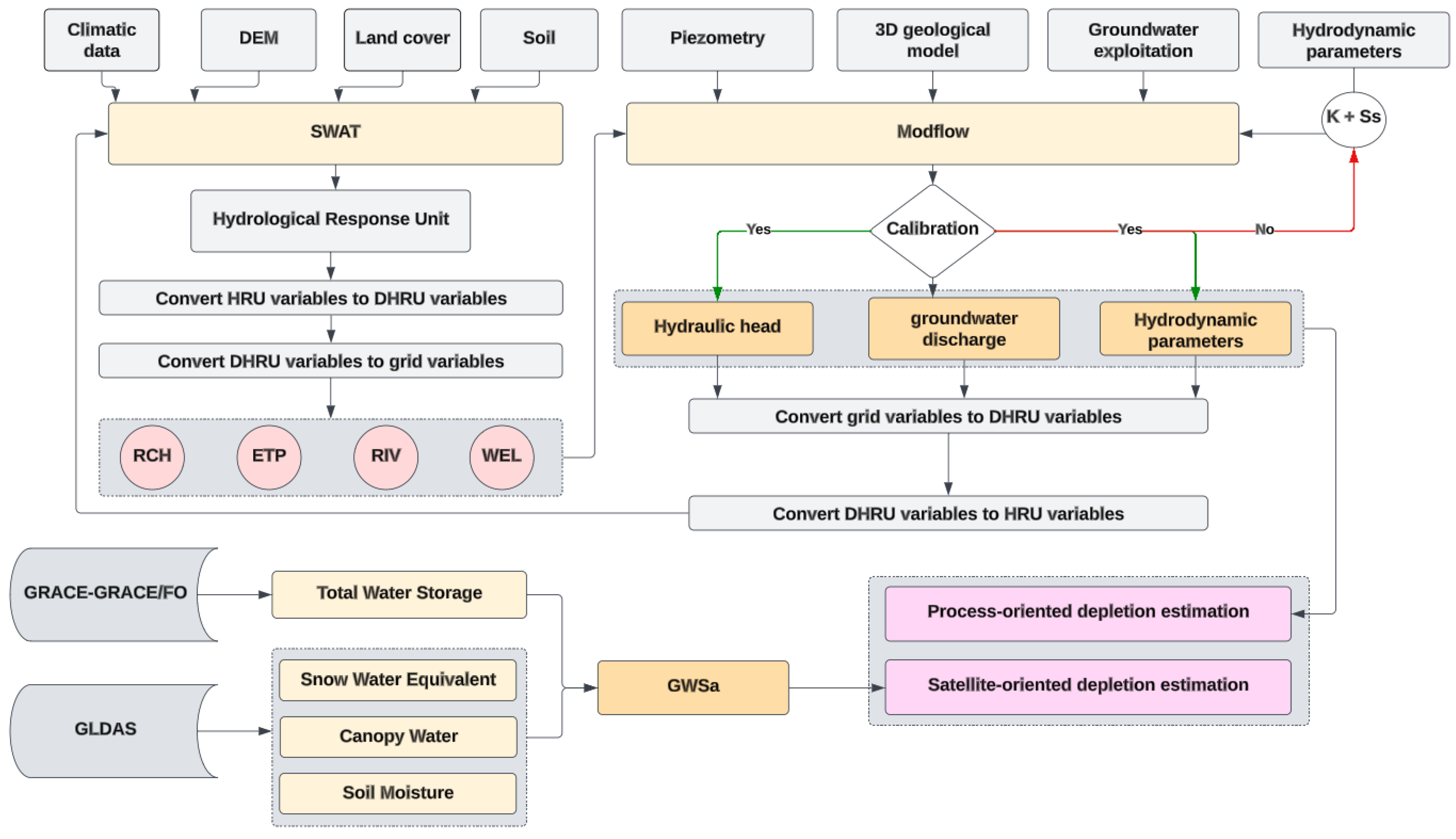
The overall research methodology can be divided into three major steps, according to the specific objectives, including (i) groundwater depletion estimation using the coupled SWAT-MODFLOW model, (ii) groundwater depletion estimation using GRACE and GRACE-FO, and (iii) the comparison and analysis of retrieved groundwater depletion variations. The overall process is summarized in Figure 2. Prior to these different steps, the meticulous task of pre-processing and harmonization of the various in situ and remote sensing data that were collected was conducted to construct the database that was required for groundwater estimation from both process-oriented and satellite-based approaches over the SRB.

As indicated in Table 1, the climatic data include precipitation, temperature, relative humidity, wind speed, and solar radiation. These data were extracted from the NASA POWER Project. The processing of these data was performed using two different codes that were developed in R to download and create the datasets that are ready for SWAT inputs.

The digital elevation model (DEM) was extracted from SRTM and processed with ArcGIS (Version 10.6.1, ESRI). The land cover map was clipped from the ESA Land Cover CCI Product, also using ArcGIS and according to the SRB limits. Soil data were extracted from the SWAT-Food and Agriculture Organization (FAO) database.

For stream data, these were exploited in the form of hydrometric information (i.e., flow and water level). These data are regularly collected by Environment and Climate Change Canada and compiled into the Hydat database. Hydat (National Hydrological Data Archive, Water Survey of Canada, ECCC) provides daily and monthly average hydrometric measurements that are collected at ground stations. In total, data from 102 stations were downloaded through the Hydat interface.

4.1. Groundwater Storage Variation from a Coupled SWAT-MODFLOW Model

This section describes the steps that were followed to reach Specific Objective 1 of the research regarding the implementation of the coupled model for estimating groundwater variation.

4.1.1. SWAT Model Set-Up

SWAT and MODFLOW are two widely used computer models for simulating water and nutrient flow in watersheds and aquifers, respectively. The combination of these two models provides a comprehensive framework for simulating and analyzing water resources management and planning. In a SWAT-MODFLOW coupling framework, the output of the SWAT model (e.g., surface water flow and water quality) can be used as inputs to MODFLOW; the results of MODFLOW (e.g., groundwater levels and spring flow) can be used as inputs to the SWAT model. This integration allows for a more accurate and comprehensive simulation of water flow and water quality changes in both surface water and groundwater systems.

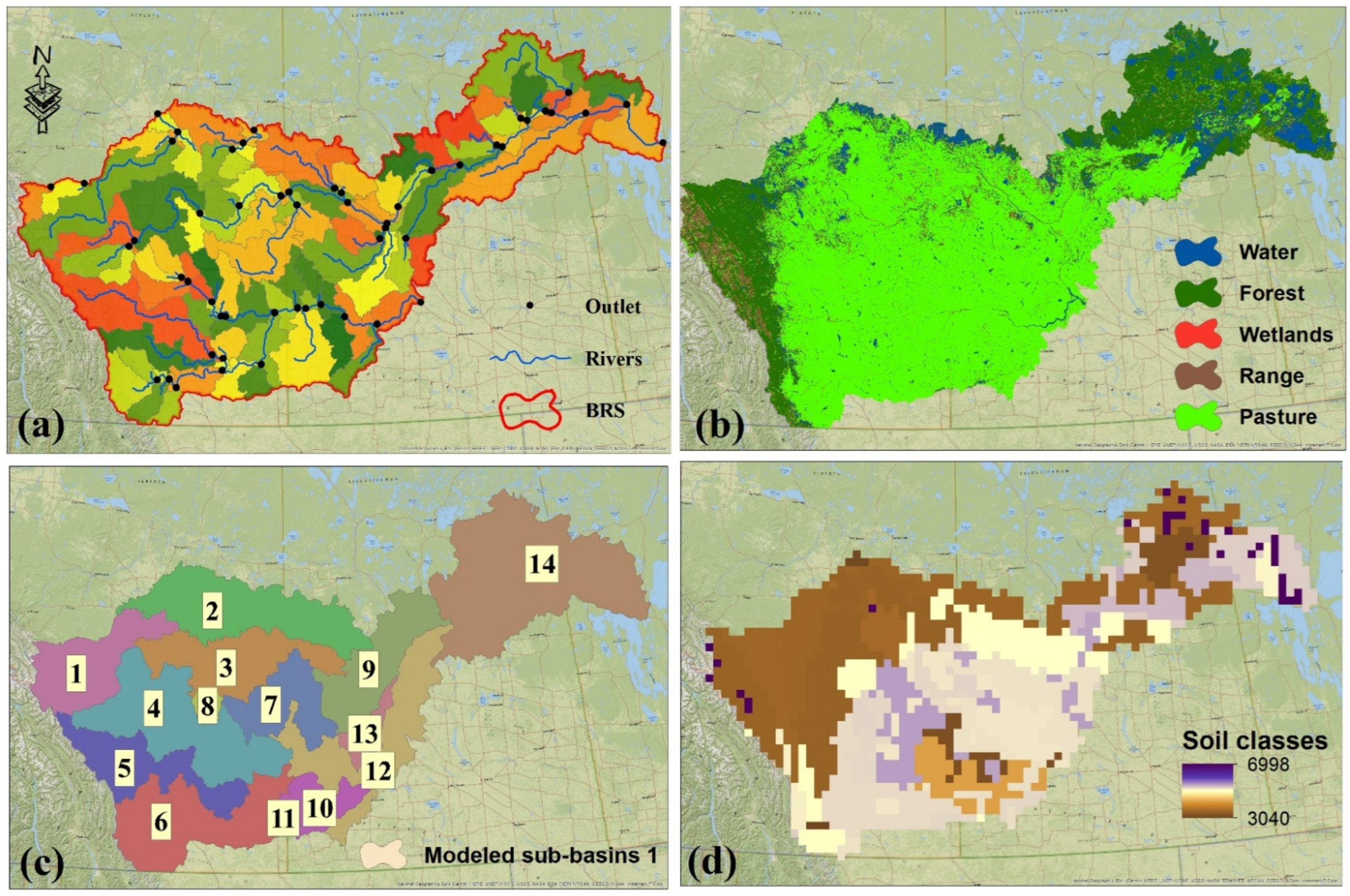
For hydrological modelling by SWAT, we used the ArcGIS-ArcView extension and interface (with SWAT) ArcSWAT 24 version. This version is incorporated into ArcMap 10.6 and works with SWAT 2012.10.6. As mentioned in Section 2, inputs to the SWAT model include topography, land use, soil texture and lithology, climate data, and water bodies (lakes and reservoirs, among others). Division of the SRB into sub-basins was accomplished after resampling the DEM (30 m) to yield 14 sub-basins (Figure 3c). The land use map that was extracted from ESA (Land Cover CCI Product) data and the soil map that was extracted from the FAO-SWAT database were used to define the hydrological response units (HRUs). The slope map was reclassified into 3 classes (<2%, 2–6%, >6%). For the land cover data, two land use maps were used: the first one was for the period 2002–2010 and the second one was for 2010–2019. Based on the combination of land use, soil, and slope, the watershed was discretized into 179 HRUs (Figure 3a).

As shown in Figure 3b, the land cover classes are identified according to the SWAT classification: Open Water (WATR), Mixed Forest (FRST), Pasture (PAST), and Vegetation (RNGE) (Figure 3b). The snow and wetland classes were not considered given their minimal areas. Most of the SRB is occupied by pasture, for more than 70% of its total area. At the same time, most of this area has a slope of <3%. Therefore, we are in a flat area of plateau type. It is dominated by grazing areas.

SWAT modelling in the SRB allows separate prediction of runoff for each HRU with routing to obtain total runoff for the watershed. This increases the accuracy and gives a much better physical representation of the water balance of the basin.

4.1.2. Groundwater Modelling Using MODFLOW

For groundwater modelling, MODFLOW-2000 was used (Harbaugh et al., 2000). The MODFLOW hydrogeologic sheet model is a finite-difference algorithm. The combination of all recognized physical laws that are necessary to represent the flow phenomenon, for the same elementary volume, yields the fundamental equation of motion or the diffusivity equation (Harbaugh et al., 2000). The equation is written as:

$$\frac{\delta }{\delta x}\left(K_{xx}·\frac{\partial h}{\partial x}\right)+\frac{\partial }{\partial y}\left(K_{yy}·\frac{\partial h}{\partial y}\right)+\frac{\partial }{\partial z}\left(K_{zz}·\frac{\partial h}{\partial z}\right)=S_s·\frac{\partial h}{\partial t}+\omega$$

(1)

where K is the hydraulic conductivity tensor, h is the piezometric rating, S_s is the specific storage coefficient, and ω is the volumetric flux per unit volume of sources and (or) sinks of water.

The diffusivity equation with added boundary conditions is a mathematical representation of the groundwater flow system. A solution to this equation, in the analytical sense, is a function h = h (x, y, z, t). Except for a few simple systems, analytical solutions to this equation are rarely possible; hence, several numerical methods are adapted to obtain an approximate solution to the problem [30]. One approach is the finite-difference method, in which the continuous system that is described by the equation is replaced by an arrangement of discrete values in space and time; the partial derivatives are replaced by terms that are calculated from the difference between values of the piezometric elevations at these points. These processes ultimately result in a linear system in which the unknowns are the piezometric ratings [15]. Put quite simply, the diffusivity equation governing flow in heterogeneous and anisotropic media is solved by the finite-difference method, whereby the flow domain is divided into blocks in which the hydrodynamic properties are assumed to be uniform. The system of equations resulting from the flow equation and its application to the whole domain can be solved by different numerical methods, which are implemented in MODFLOW [15]. These include the preconditioned conjugate gradient method [31], preconditioned Cholesky method, or Strongly Implicit Procedure [32].

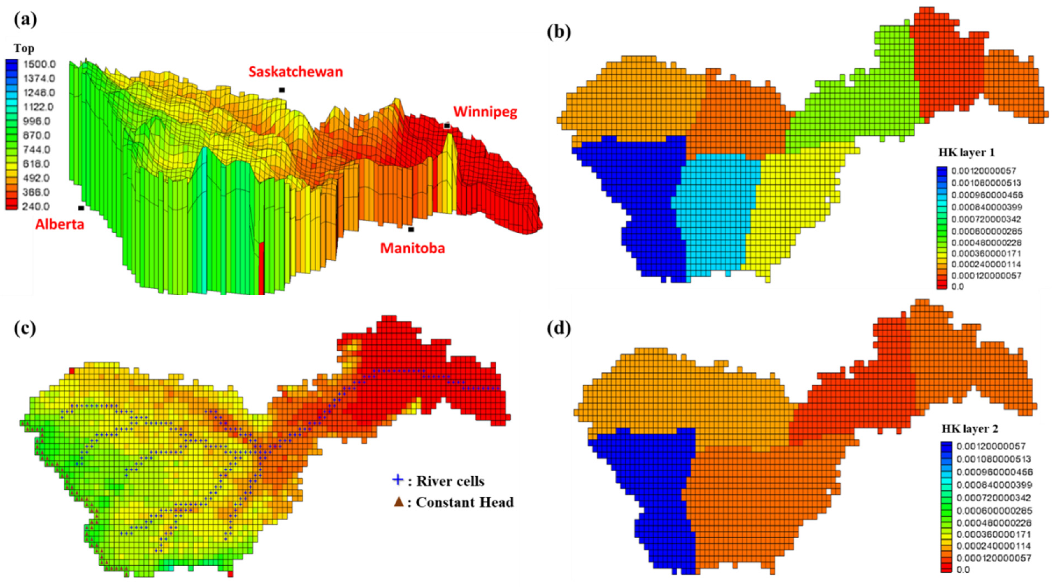
Modelling was performed using Groundwater Modeling System-GMS 10.0 software (Aquaveo LLC, Provo, UT, USA), which allows the simulation of water and contaminant transfers in a multilayer system based upon the finite-difference method. The modelling domain is inscribed in a matrix of 50 columns and 100 rows, i.e., 5000 square and regular meshes of 25 km to the side. The model is composed of two aquifer layers (K = 2): (i) The first layer refers to the surface horizon (Figure 4a,c). It represents the water table that is captured by the surface wells. (ii) The second layer includes all deep horizons, i.e., the two permeable levels that are contained in the Paskapoo, Horseshoe Canyon, and Oldman Formations.

These formations were chosen based on the availability of exploitation data and the availability of a 3D geological model that was developed by [33]. This model was constructed using an implicit 3D method based upon the integration of data from hydraulic boreholes, oil boreholes, surface geology, cross-sections, and a DEM. The geometry of the geological layers is characterized, which allows us to estimate variation in the thickness of the aquifer layers. This model has been exported in GRID format and has been very smoothly integrated into the GMS.

As shown in Table 1, many sources of remote sensing data were used in the modelling work. In fact, on the north portion of the modelled region, the Snow Water Equivalent (SWE) values that were extracted from the North American Regional Reanalysis data (National Centers for Environmental Prediction, NOAA) were integrated as a Constant Head (CHD) boundary condition. The river discharge (RIV package, MODFLOW) and recharge rates (RCH package, MODFLOW) estimates were integrated directly from the SWAT model outputs.

In the first phase, the model was calibrated in a steady state for the year 2002. This consists of simulating a quasi-stationary state of the system, which is not influenced by withdrawals from the aquifer. Steady-state calibration ensures consistency between transmissivity (m²/s) and the boundary conditions that were adopted by the model. In the second step, the model is calibrated in a transient regime (from 2003 to 2019). To do this, the model simulation was performed over a historically known period during which the system has undergone strong disturbances that are related to withdrawals. Comparison of calculated piezometric results with the observed series allows us to judge the degree of representativeness provided by the model that was developed.

Since there is no known reference state with good accuracy over the whole domain, the calibration procedure that was adopted consisted of simulating the behaviour of the model in a steady state by mainly adjusting the horizontal and vertical transmissivities, checking that the piezometric map that was obtained agrees well with the observed one, adapting the initial conditions to simulate the model for the 2002 period, and then comparing the calculated and observed piezometric series. When the piezometric evolution is not reconstituted at the level of a piezometer in spite of modifications that were applied to the coefficient of storage, we return to the computation in a steady state to readjust the transmissivities or the coefficient of drainage in the zone in question. The transient calculation is then repeated until the calibration is satisfactory.

4.1.3. Coupling SWAT-MODFLOW

The SWAT-MODFLOW coupling is based on a sequential transmission procedure between SWAT (HRU) and MODFLOW (GRID) computing units. The hydrological flows are transmitted in daily order, day by day, from the HRUs to the GRIDs and from the GRIDs to the HRUs. Readers can find a tutorial for using ArcMap routines to link SWAT (RHU, sub-basins) and MODFLOW (grid cells) computational units at the following link: https://swat.tamu.edu/software/swat-MODFLOW/ (accessed on 10 August 2023). Two software tools also have been published to automate model coupling and model simulations, thereby limiting human error and decreasing preparation time. SWATMOD-Prep [33,34] uses a standalone Python script to perform the necessary geographic couplings and prepare the necessary input files. QSWATMOD [34] is a QGIS plug-in tool that reads SWAT shapefiles, reads or creates MODFLOW shapefiles, performs spatial linkage operations, writes linkage input files, runs SWAT-MODFLOW simulations, and provides visualization tools for stream hydrographs, groundwater levels, groundwater budget fluxes (recharge, groundwater, and surface water exchange), and watershed-scale temporal water budgets.

In this study, we used the SUFI-2 (Sequential Uncertainty Fitting) algorithm implemented in the SWAT-CUP tool to calibrate and validate the SRB model, and to assess the uncertainty. The SWAT model calibration was done considering both the relative and replace modes.

Table 2. SWAT- MODFLOW model calibration parameters.

Calibration Parameters	Definition	Initial Interval	Calibrated Value
Relative mode
CN2	Initial SCS runoff curve number for moisture condition II	[−0.75–0.75]	−0.641
OV_N	Manning coefficient of the river network as a whole	[−0.5–0.5]	−0.117
Sol_AWC	Available water capacity in the soil layer	[−0.5–0.5]	−0.4810
GW_Delay	Aquifer recharge time	[−0.15–0.15]	−0.0314
Replace mode
SURLAG	Runoff delay coefficient	[−0.25–0.25]	0.1421
Sol_K	Hydraulic conductivity at saturation	0–500	274.1420
GWQMN	Groundwater contribution threshold to channel flow, baseflow	0–5000	3901.2214
GW_Revap	Evaporation coefficient from groundwater	0.02–0.2	0.14570
RCHDP	Coefficient of percolation to the deep-water table	0–1	0.02134
CH_N2	Manning coefficient of principal channels	0.02–0.06	0.05115
CH_K2	Permeability of the banks of the main canals	20–200	241.3640
EPCO	Plant factor of soil evaporation as a function of depth	0–1	0.7994
Alpha_BF	Groundwater depletion coefficient	0.95–1	0.91147

defines the calibration parameters in each mode. In total, 20 iterations and 1000 simulations were performed. This number of iterations is considered important in SWAT modelling, but it was necessary due to the vastness of the basin and the large number of sub-catchments. Finally, after parameter calibration, variations in the coefficient of determination (R²) and the percentage of measured data that were bracketed by the 95 percent prediction uncertainty (p-factor) were used to assess model performance (see Section 4.4 for performance metrics). The final model was calibrated for the 2002–2014 period and validated for the 2015–2019 period.

Groundwater Storage variation GWS(SWAT-MODFLOW) was calculated using the approach of Iqbal et al. (2016). This approach is based on two important steps: (i) SWAT-MODFLOW simulated piezometric levels are transformed into Groundwater Piezometric Level anomalies (GPLa) by subtracting the average of variations between 2002 and 2019. (ii) The variation of GWS anomalies is then calculated by multiplying the GPLa by the specific yield (Sy) that is calibrated by MODFLOW. This approach is also applied to the observed piezometry.

4.2. Groundwater Storage Variations from GRACE/GRACE-FO Data

The methodology in this section responds to specific objective 2. GRACE and GRACE/FO TWS anomalies have been processed by different centres; CSR (UT Center for Space Research), GFZ (German Research Centre for Geosciences), and JPL (Jet Propulsion Laboratory) (Landerer and Swenson, 2012). TWS consists of surface and sub-surface storage compartments, such as snow water equivalent, surface water, soil moisture, snow, groundwater, and canopy water (Chen et al., 2016). The GRCTellus Land RL06 release of GRACE and GRACE/FO data from these centres is available in two different solutions, i.e., spherical harmonic and mascon (Mass Concentration blocks). We used JPL monthly spherical harmonic solution data, which are available at 1° × 1° resolution from 2002 to 2019 (https://grace.jpl.nasa.gov/data/get-data/monthly-mass-grids-land/ (accessed on 10 August 2023)). Months for which GRACE observations were missing were filled by linear interpolation and by averaging the values of two months before and after the month with missing data, as suggested by previous studies (Long et al., 2015; Ali et al., 2021). A scaling factor was applied to restore the original signal in GRACE data that was lost during the pre-processing [35].

Given that TWS is a single integrated quantity including the different water components, it is necessary to use other sources of data to isolate and estimate groundwater anomalies from it. Hydrological models are often used for that purpose. In this study, we used the Global Land Data Assimilation System (GLDAS) to extract the other water balance parameters, i.e., soil moisture (Hsol), snow and ice water equivalent (SWE), and canopy water (WCan). These parameters were then converted into anomalies, i.e., the differences between the monthly averages and the average over the whole period of the time series in each case. Finally, groundwater anomalies (GWS) were computed based on the balance equation [36], where:

$$\mathrm{T}\mathrm{W}\mathrm{S}=\mathrm{G}\mathrm{W}\mathrm{S}+\mathrm{H}\mathrm{s}\mathrm{o}\mathrm{l}+\mathrm{S}\mathrm{W}\mathrm{E}+\mathrm{W}\mathrm{C}\mathrm{a}\mathrm{n}$$

(2)

Note that all components in the equation are anomalies. Thus, GWS could be estimated as:

$$\mathrm{G}\mathrm{W}\mathrm{S}=\mathrm{T}\mathrm{W}\mathrm{S}-\left(\mathrm{H}\mathrm{s}\mathrm{o}\mathrm{l}+\mathrm{S}\mathrm{W}\mathrm{E}+\mathrm{W}\mathrm{C}\mathrm{a}\mathrm{n}\right)$$

(3)

GWS was validated using observational data that were taken from piezometric wells in the region. These data are available in the form of piezometric levels (GPL). For the purpose of the study, we converted GPL into groundwater storage variations (GPLa) by applying the same approach that was proposed by Iqbal et al. (2016). This approach was also used to estimate GWS anomalies from SWAT-MODFLOW (see Section 4.3).

4.3. Depletion from SWAT-MODFLOW and GRACE/GRACE-FO Data

Depletion can be calculated using coupled SWAT-MODFLOW model outputs for each Budget Zone as well as from the GRACE-GRACE/FO data. The general steps for calculating the average depletion are as follows:

First, it is important to identify the well or piezometer locations for each budget zone in which depletion is to be calculated and average the piezometry variations for the budget zone using SWAT-MODFLOW.

Inter-monthly depletion for each budget zone can be calculated by taking the difference between initial and final water table levels and dividing this result by the duration of the simulation (here, equal to 1 month):

$$Depletion (in mm per month)={GPLa}_i-{GPLa}_{i-1}$$

(4)

where GPLa is groundwater piezometric level anomalies, which were extracted from observed data or SWAT-MODFLOW or GRACE data, and i is a monthly counter from April 2002 to December 2019.

4.4. Performance Metrics

The following accuracy metrics evaluated the performance of the different observed and simulated flows (outputs of SWAT), together with the observed and simulated heads (outputs of MODFLOW): coefficient of determination (R²), Nash-Sutcliffe efficiency (NSE; [37], and percent BIAS (PBIAS). These three metrics are computed as follows:

$$R^2=\left(\frac{{\sum }_{i=1}^N\left[\left(X-(\sum _{i=1}^{N}P/N\left)\right)\times (X_{simulated}-(\sum _{i=1}^N{X}_{simulated}/N\right))\right]}{\sqrt{{\sum }_{i=1}^N\left[{\left(X-(\sum _{i=1}^{N}X/N)\right)}^2\times {(X_{simulated}-(\sum _{i=1}^N{X}_{simulated}/N\left)\right)}^2\right]}}\right)$$

(5)

$$NSE=1-\left[\frac{\sum _{i=1}^N{\left(X_{}^i-X_{simulated}^i\right)}^2}{\sum _{i=1}^N{\left(X_{}^i-X_{mean}^{}\right)}^2}\right]$$

(6)

$$PBIAS=\left[\frac{\sum _{i=1}^n{\left(X_{}^i-X_{simulated}^i\right)\times 100}^{}}{\sum _{i=1}^n{\left(X_{}^i\right)}^{}}\right]$$

(7)

where X_simulated is the simulated flow, X is the observed flow, $X_{mean}^{}$ the mean between the observed and simulated value, i is a counter and N is the number of data points.

Furthermore, the p_factor was used to quantify uncertainties between observed and simulated flows and is defined as the percentage of observed data framed by the 95% prediction uncertainty (95 PPU). The 95 PPU is calculated at the 2.5% and 97.5% levels of the cumulative distribution of an output variable that are obtained by Latin hypercube sampling. In other words, it is calculated from the 2.5 and 97.5 percentiles of the cumulative distribution for each simulated point.

5. Results

5.1. Groundwater Storage from the Coupled SWAT-MODFLOW

5.1.1. SWAT Model Calibration and Validation

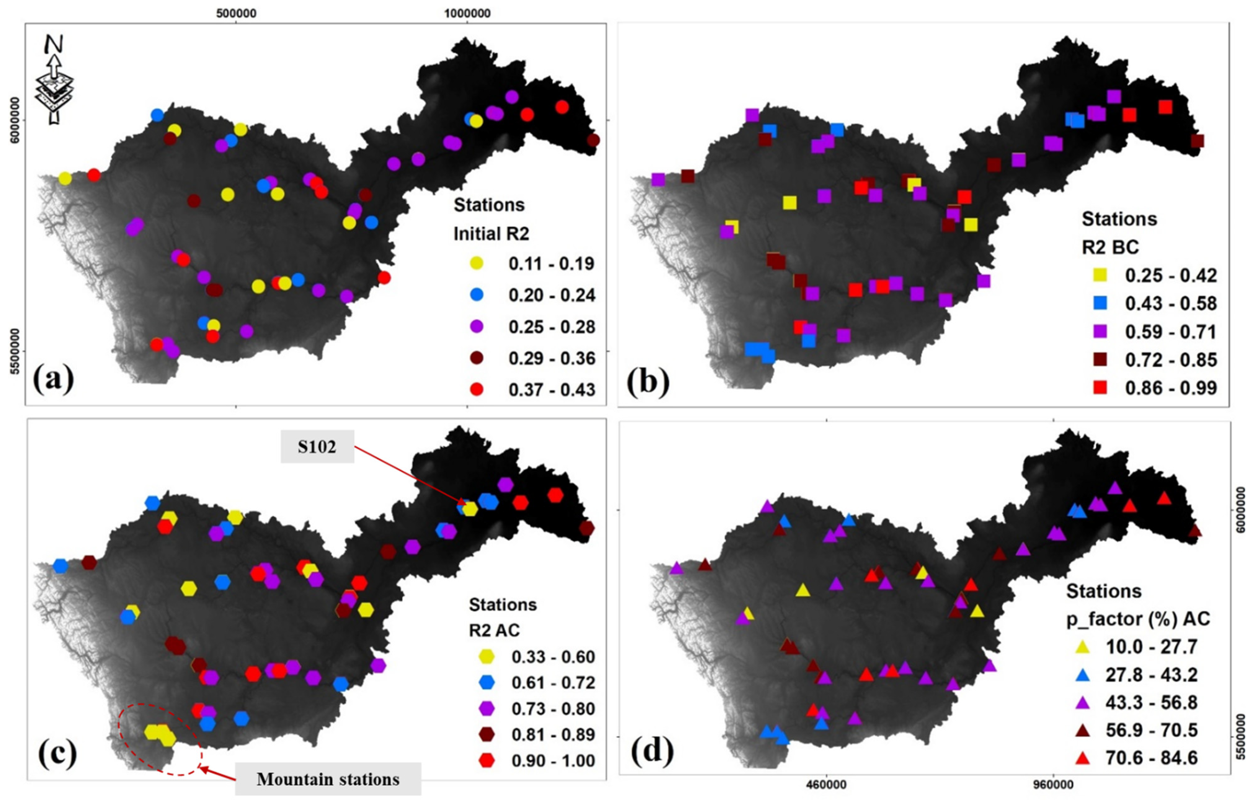
First, the SWAT model was run without calibration, and the simulated river flows were compared to the observed flows that were extracted from the Hydat hydrometric database. Figure 5 summarizes the performance metrics: (5a) initial R² prior to SWAT calibration and coupling; (5b) R² after SWAT calibration and before coupling; (5c) R² after calibration and after coupling with MODFLOW; and (5d) p_factor after coupling.

As shown in Figure 4, the model (prior to calibration) exhibits R² values between 0.11 and 0.43, with an average of 0.27 between observed and simulated flows. To improve the SWAT model’s estimates of river discharge, a multi-station and multi-objective calibration was performed before coupling. Following this exercise, the model calibration results show R² values ranging from 0.25 to 0.99 between observed and simulated flows. Most of the SRB stations that were considered (68%) show significant R²-values ranging from 0.59 to 0.99, with an average value of 0.79. This shows that the multi-station calibration attempts were successful and that the SWAT model appropriately reflects the precipitation, runoff, water percolation, and groundwater recharge regime of the SRB. Yet, 12% of the stations exhibited low R²–values (between 0.25 and 0.42; i.e., not statistically significant) despite multiple calibration attempts. Further investigation will be undertaken to better understand the local hydrological processes over these stations.

At the beginning of the calibration work, three stations (southwestern region of the basin, within the Rocky Mountains, AB; Figure 5c) showed poor performance. During calibration, several tests were performed to determine the sensitivity of these stations to climatic parameters. They are influenced by temperature, although the area is dominated by snowfall. Therefore, we adjusted the snowmelt factor and found a considerable improvement in R² for these stations (i.e., between 0.43 and 0.58).

A possible source of uncertainty in our SWAT modelling may be linked to the integration of data that are related to water bodies (dams and lakes). Due to their important role in regulating surface runoff, we were able to incorporate 19 dams into the model. The choice of the dams was based on the proximity of the hydrometric station, their important role in total runoff, and the availability of a continuous long-term hydrometric dataset. We noticed an improvement in estimates of the stations, which are downstream of the dams, but no improvement for the mountainous stations.

5.1.2. MODFLOW Calibration and Validation

The piezometric level that was simulated by MODFLOW was calibrated using 27 piezometers that had a continuous record from 2002 through 2019. The stations that were used for the SWAT model calibration are also integrated into the MODFLOW model to define water levels in the different rivers of the SRB.

Figure 5 presents the calibration results.

The first calculations show a piezometric level in the first layer that was strongly influenced by the piezometric level of the second layer. This is a consequence of the increasing exploitation of groundwater in the Province of Alberta. We further reduced the vertical connection between the two layers over the entire domain except in the northern part of the basin, which lies in the Province of Saskatchewan, where the two water tables are merged. After about ten tests during which transmissivity and the drainage coefficient were modified, the calculated piezometric maps showed a pattern similar to the reference piezometric levels for both modelled layers; therefore, the calibration process was stopped (Figure 5a).

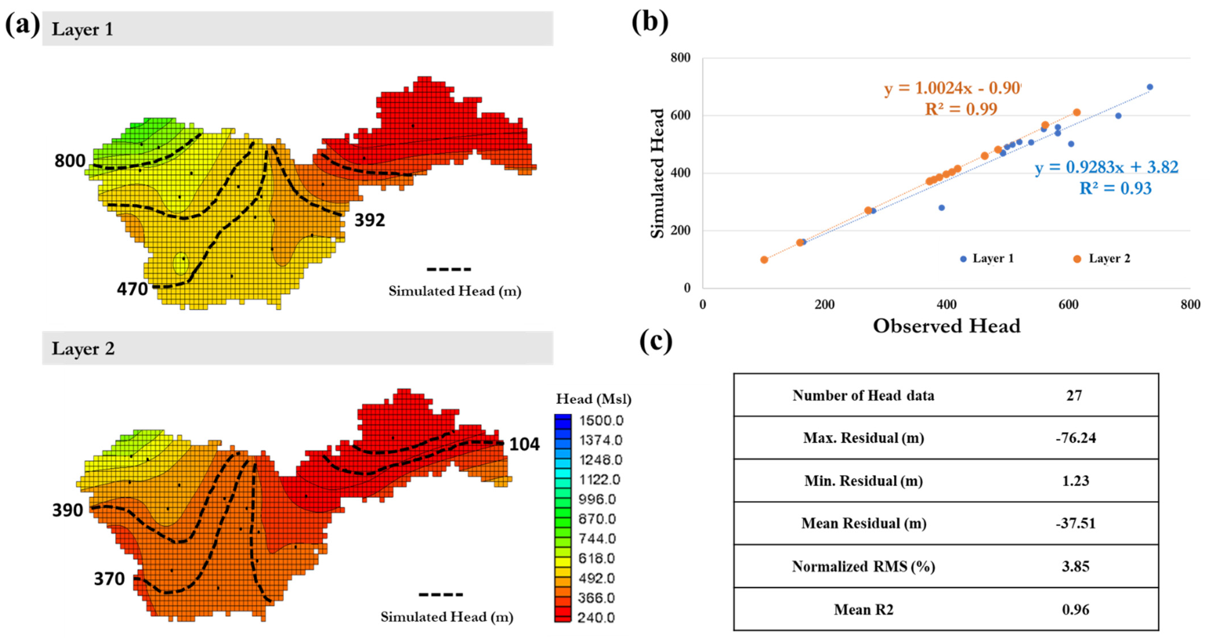
The performance metrics that were used to evaluate the calibration of the MODFLOW model show an accurate calibration (Figure 6b). The best statistical metric values are found on the Saskatchewan plain: mean R² = 0.96, and mean residual was equal to −37.5 m (Figure 6c). These values are considered sufficient for the evaluation of a robust and realistic model [37,38,39]. Yet, these values could be improved after coupling with SWAT.

Figure 6 shows the spatial variation in the observed and simulated piezometry for the year 2002 for the two modelled layers. The variation shows that the isopieces (i.e., lines of equal groundwater pressure) of layer 1 are spaced apart and that the hydraulic gradient is average. The layer 1 piezometric map for this layer shows that the flow of water from the water table generally follows a main NW-SE direction. The direction of groundwater flow coincides substantially with the direction of surface water flow that drains the watercourse following the topographic slope. The isopiece curves are generally convex, indicating a linear supply from the streams. Towards the north of the sector, the isopiece curves are tightly spaced. The hydraulic gradient is on the order of 7‰. This curve pattern reflects good water circulation, witnessing good transmissivity of the land, amplified by the slope of the land. The hydraulic gradient of this water table becomes steadily weaker as it moves toward the centre (Figure 6), down to about 4 ‰. Towards the southeast, in the area around Saskatoon (SK), the piezometric level coincides with the topographic surface in the vicinity of Lake Winnipeg (MB), indicating its emergence.

The simulated piezometric map for Layer 2 (Figure 6a) shows that groundwater flow generally follows a major direction, NS and WE. The direction of groundwater flow coincides substantially with the direction of surface water flow that drains the stream following the topographic slope. To the northwest, the isopiece curves are tight due to a high hydraulic gradient of about 21‰ (Figure 6). Towards the northeast, the curves become increasingly more widely spaced. From Saskatoon (SK), the spacing between curves becomes very large with a hydraulic gradient equal to 1‰ (Figure 6). These variations in hydraulic gradient are thought to be due primarily to heterogeneity in the lithology and reduction in the thicknesses of the deep-water table in the area.

5.1.3. Coupling SWAT-MODFLOW

The coupling of SWAT and MODFLOW was performed according to the approach that was presented in Section 4.1.3. The results of the performance metrics are shown in Figure 5. After coupling, the R²-values improved with the range of variation explained shifting from 0.25–0.99 to 0.33–1.00. The mountainous stations (in yellow in Figure 5c) show slight improvements (R² between 0.33 and 0.60). Station S102 (see location in Figure 5c) showed degradation in calibration quality following coupling (R² decreased from 0.54 to 0.42). In fact, S102 is the only station that exhibited degradation in calibration quality between the observed and simulated flow. This degradation is mainly related to the hydrogeological nature of this region where layer 1 and layer 2 are geologically communicating. The p-factor values after coupling vary between 10 and 85%, showing that the SWAT-MODFLOW model was ready to be used to quantify the water balance and the variation of aquifer storage.

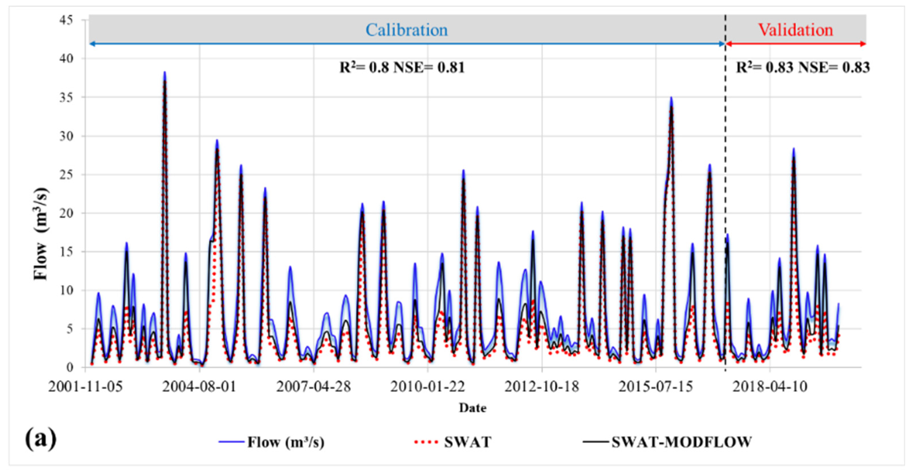
For illustrative purposes, two gauging stations are selected to exemplify and discuss the calibration quality of the SWAT-MODFLOW model (

Table 3. Characteristics of the selected gauging stations.

Gauge Name	Latitude	Longitude	Drainage Area (km2)	Regional Office
Deep valley creek near Valleyview, AB	54°25′49.7″ N	117°43′16.7″ W	635	Calgary
Smoothstone River below Emmeline Lake, SK	55°9′48.0″ N	106°12′25.0″ W	6020	Regina

). The stations were chosen according to their drainage area and performance metrics.

Figure 7 shows the monthly observed and simulated SWAT and SWAT-MODFLOW flows for the selected. Figure 6a represents the results for a gauging station with a low drainage area (635 km²). It shows a good calibration and validation result (R² = 0.83 and NSE = 0.83). The peaks at this station representing flood flows are well estimated for most events. Low water flows are better represented but with a certain lag of ±1.71 m³/s. At the time of the calibration attempts, some parameters could be varied, such as SURLAG, CN2, and RCHDP. Increasing these parameters leads to an increase in the flood flows, which will be overestimated. Thus, exaggerated values of these flows will lead to increased runoff and decreased recharge of aquifers; this creates a contradiction with respect to the typical behaviour of the basin. If we accept the underestimation of baseflows, this would lead to a considerable increase in the performance indices (R², NSE). Therefore, we accepted the underestimation conditions for this station, which we consider acceptable according to the conceptual model that was established for the SRB. In addition, SWAT-MODFLOW showed marked improvement in calibration results compared to SWAT. For this type of gauge with a limited drainage area, our coupled model is able to reproduce the flow correctly and more accurately than with SWAT alone.

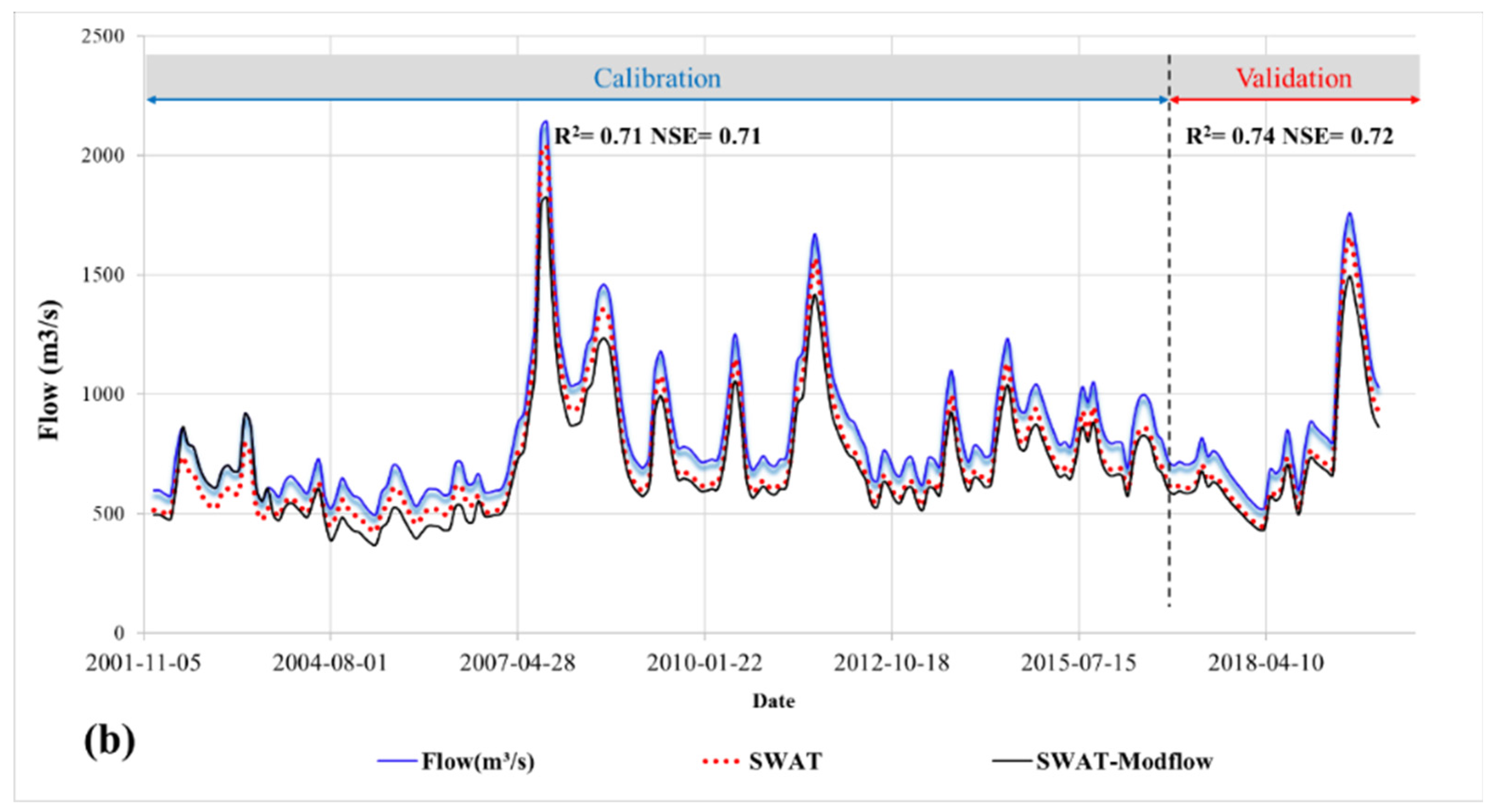
Figure 7b shows the case of a station with a large drainage area (6020 km²). The calibration and validation results show less interesting, but statistically significant performance metrics (R² = 0.74 and NSE = 0.72). The SWAT model in this case appropriately represents the observed flows, but we note degradation in the results after coupling. The SWAT-MODFLOW model more poorly translates the observed flows for this case with an important drainage area.

Among the outputs of the coupled SWAT-MODFLOW model, we show evapotranspiration, runoff, soil moisture, groundwater recharge, and deep groundwater recharge in Figure 8. The most important simplification to the study is applied to the spatial resolution of the MODFLOW mesh, i.e., 25 km by 25 km. Yet, we must consider the potential effects of the uncertainties that may be introduced and related to SWAT-MODFLOW model inputs when interpreting the results.

The values shown in Figure 8 are aggregated for each modelled sub-basin at a monthly time step from 2002 to 2019. At first glance, the SRB sub-basins do not function in the same way according to the modelling results. In fact, evapotranspiration (Figure 8b) shows a similar trend to simulated precipitation in the mountainous part of the SRB but a less pronounced trend in the central part of the basin. For the nearby Lake Winnipeg, there are no similarities between evapotranspiration and precipitation. The high values (between 42.1 and 46.9 mm) in this area are mainly related to mixed and coniferous forests, and to the conspicuous presence of wetlands in this region. In the centre of the SRB, there are still important values of evapotranspiration (between 34.8 and 42 mm) given major agricultural activity (Figure 8b).

For example, runoff varies from 1.98 to 14.2 mm in the northern part of the SRB (Figure 8c). This response is mainly due to the changing slope from mountainous areas to the Canadian prairie plains. Soil moisture subsequently varies between 34.5 and 45.6 mm. Its variations are influenced by the presence of forest and snow cover. The highest values occur in the mountainous areas that are dominated by the presence of snow. Soil moisture levels are also high in the central region, where there are extensive irrigated areas. Minimum soil moisture is observed in the northern SRB that is covered by forests (34.5–45.6 mm, Figure 8d). The topography of the area could also have an influence here. Slopes can have a thinner layer of soil due to erosion, which can reduce soil moisture.

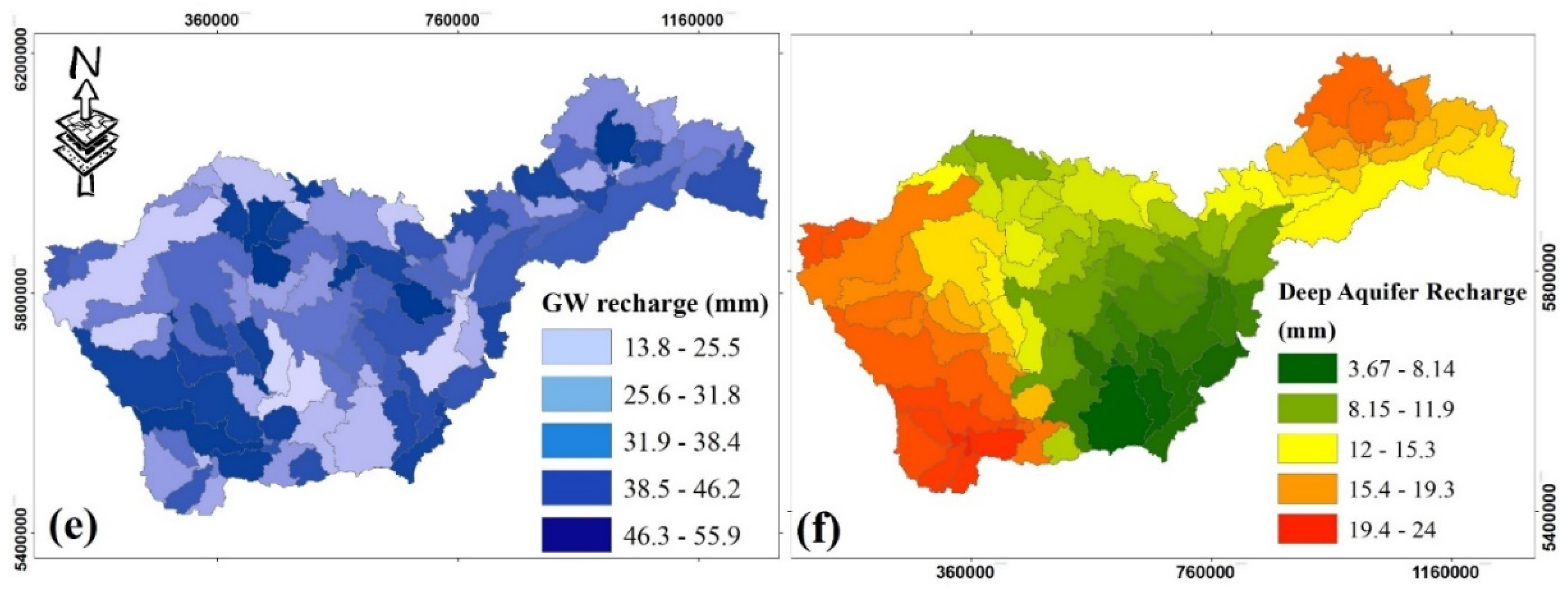
For recharge, the SWAT model simulates groundwater recharge and deep aquifer recharge (Figure 8e,f). The quantity of water entering the aquifers is discharged into the rivers in the form of vertical flows if piezometric conditions are favourable. The recharge map of the superficial aquifers shows heterogeneity at the level of the modelled sub-basins. This recharge varies between 13.8 and 55.9 mm. Indeed, the recharge process depends not only upon all of the parameters mentioned above (evapotranspiration, runoff, and soil moisture) but also on the snow water equivalent, which is translated here into the runoff. We also note that topography plays an important role in recharge. Areas at higher elevations often have steeper slopes and may exhibit faster groundwater recharge. It should also be remembered that some soils have limited storage capacity and, hence, limited recharge.

Recharge values for deep aquifers range from 3.67 to 24.00 mm (Figure 8f). The centre of the SRB basin shows the lowest recharge values (3.67 to 11.9 mm). The groundwater recharge maps show a large quantity of recharge in mountainous areas. This confirms that an important part of the recharge water ends up in the rivers as a vertical flow, while a minimal quantity reaches the deep aquifer. In examining the evapotranspiration map, a considerable portion (62%) of this water leaves in the form of evapotranspiration, indicating that sustainable water (water that reaches the deep aquifers) is vulnerable and could be threatened by over-exploitation.

5.2. Groundwater Storage Variation from GRACE/GRACE-FO

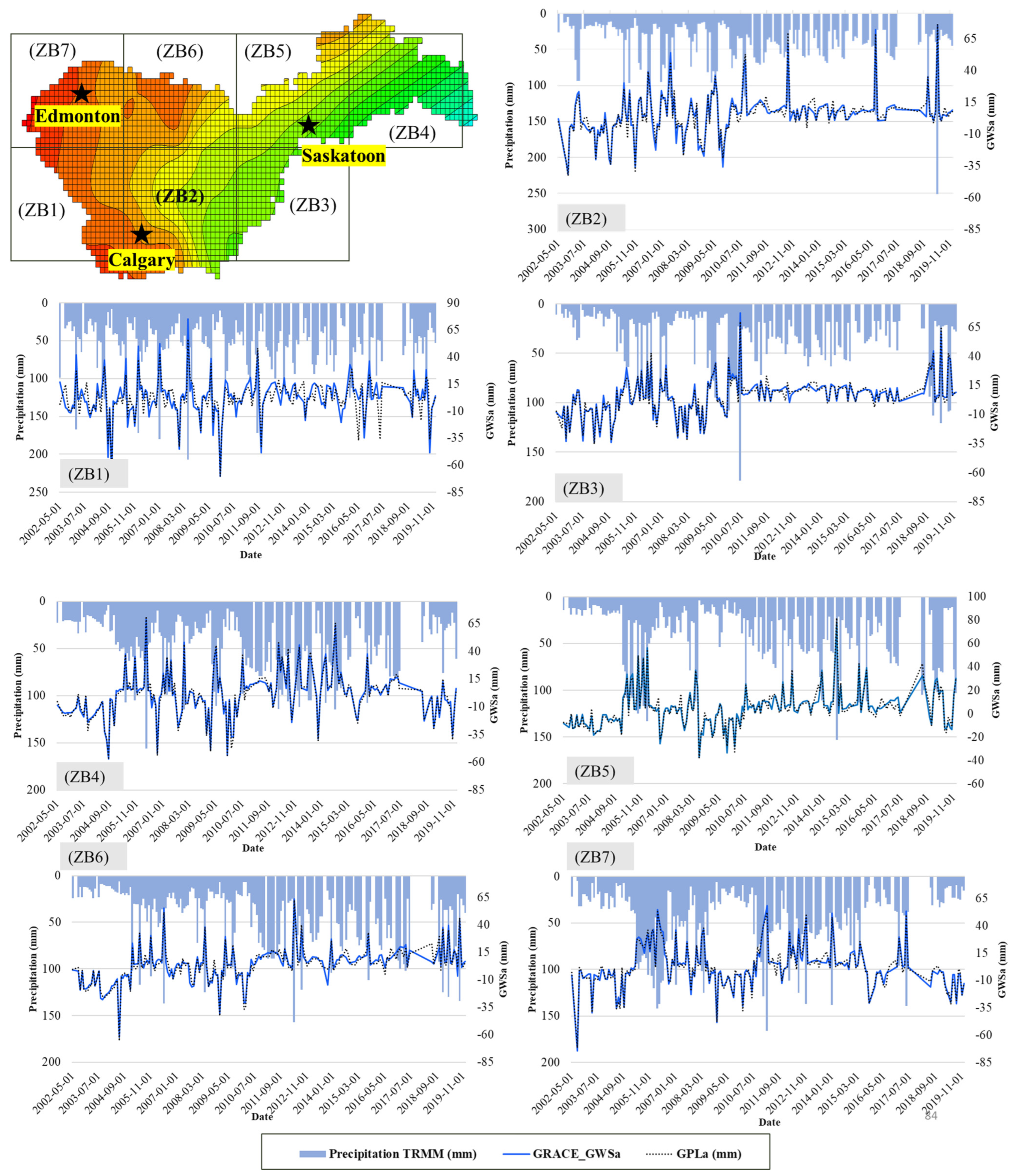
The approach that was used to estimate groundwater storage anomalies from GRACE and GRACE/FO is described in Section 4.2. Figure 9 shows a comparison between the temporal variation of GWS and in situ GPLa in the SRB using the same zone budget splitting (ZBs: 1 to 7), as was performed for SWAT-MODFLOW. Precipitation information was included in Figure 8 to help interpret the relationship between variations in GWS in the SRB.

Comparison between GRACE-based GWS and GPLa (From observed piezometry) is summarized in

Table 4. Comparison statistics between GWS from GRACE/GRACE-FO and GPLa (observed piezometry).

Zone Budget	R2 (GWS/GPLa)	NSE (GWS/GPLa)
ZB1	0.67	0.66
ZB2	0.89	0.86
ZB3	0.88	0.86
ZB4	0.90	0.91
ZB5	0.89	0.86
ZB6	0.87	0.86
ZB7	0.71	0.68

. Significant correlations were found for all budget areas, except for ZB1 and ZB7, which have the lowest values (R² = 0.67, NSE = 0.66; and R² = 0.71, NSE = 0.68, respectively). These areas are classified as recharge areas of the SRB aquifer system, which undergo the combined action of SWE and intensive groundwater exploitation; furthermore, the nature of the landscape results in medium groundwater storage potential.

The general trend in GWS variations for all zone budgets shows a sawtooth pattern (Figure 9), which confirms that the SRB not only undergoes episodes of recharge but also includes episodes of extensive groundwater drop. ZB1 corresponds to the Rocky Mountains Foothills. The moderate correlation (R² = 0.67) between GWS and GPLa (Table 3) could be explained by the steep slopes and rocky materials that are present, which in turn influences groundwater flow. Yet, the reasonable accuracy of the results (NSE = 0.66) in estimating groundwater storage variations from the piezometric water-level measurements exemplifies the potential usefulness of GRACE/GRACE-FO data in detecting groundwater storage variation.

Zone Budget ZB2 and ZB3 correspond to the agricultural plains where groundwater use is intensive. Both zones exhibit high correlation and NSE between GRACE/GRACE-FO and GPLa results, as summarized in Table 4 (R² = 0.89 and R² = 0.88, respectively; NSE = 0.86). In agricultural areas, groundwater is frequently used for crop irrigation, which can lead to over-exploitation of aquifers. Recharge of aquifers can be limited due to high precipitation, and, at the same time, high temperatures that promote evaporation more than recharge and surface runoff that prevents water infiltration into the soil. In addition, these agricultural areas include several piezometers with comprehensive data histories, which make comparisons more accurate. This suggests that the proposed method may be useful for tracking changes in groundwater storage in the agricultural plains.

ZB4 corresponds to wetlands and boreal forest transitions. Strong results that were obtained (R² = 0.90, NSE = 0.91) could be explained by the presence of an extensive network of piezometers. Zone ZB5 is influenced by high surface water pressure due to the presence of wetlands around Lake Winnipeg. Here, also there is strong concordance between GRACE and GPLa estimated groundwater storage values (R² = 0.89, NSE = 0.86). ZB6 is a transition zone to boreal forests, with moderate groundwater development. It provides results that are very similar to ZB5. Finally, ZB7 is a mountainous area, where the relationships that were found are relatively moderate and in the same order as those in ZB1 (R² = 0.71, NSE = 0.68). Mountainous conditions may make the correlation between GWS and GLPa less direct, due to the complexity of groundwater flow and storage processes [40].

The lowest GWS values were observed in summer (−80 mm in June 2002 for ZB7) and the highest values in mid-autumn (+77 mm in October 2018). Three significant groundwater droughts were observed respectively, in October 2003, December 2009, and November 2018. Compared to TRMM precipitation in the Regina area, these were attributed to the 2003, 2009, and 2018 droughts with a lag, which is consistent with the response time of the aquifer.

For the Saskatchewan region, the GWS anomalies showed several groundwater dynamics responses for all ZBs. In ZB2 and ZB3, GWS variations had a monotonic trend with a few sudden spikes. This trend could be explained by the variation between good recharge and intensive exploitation of groundwater resources in these two areas. These areas are known for their intensive agricultural activities that consume large quantities of groundwater. Given the low flow of the South Saskatchewan River, farmers use groundwater intensively.

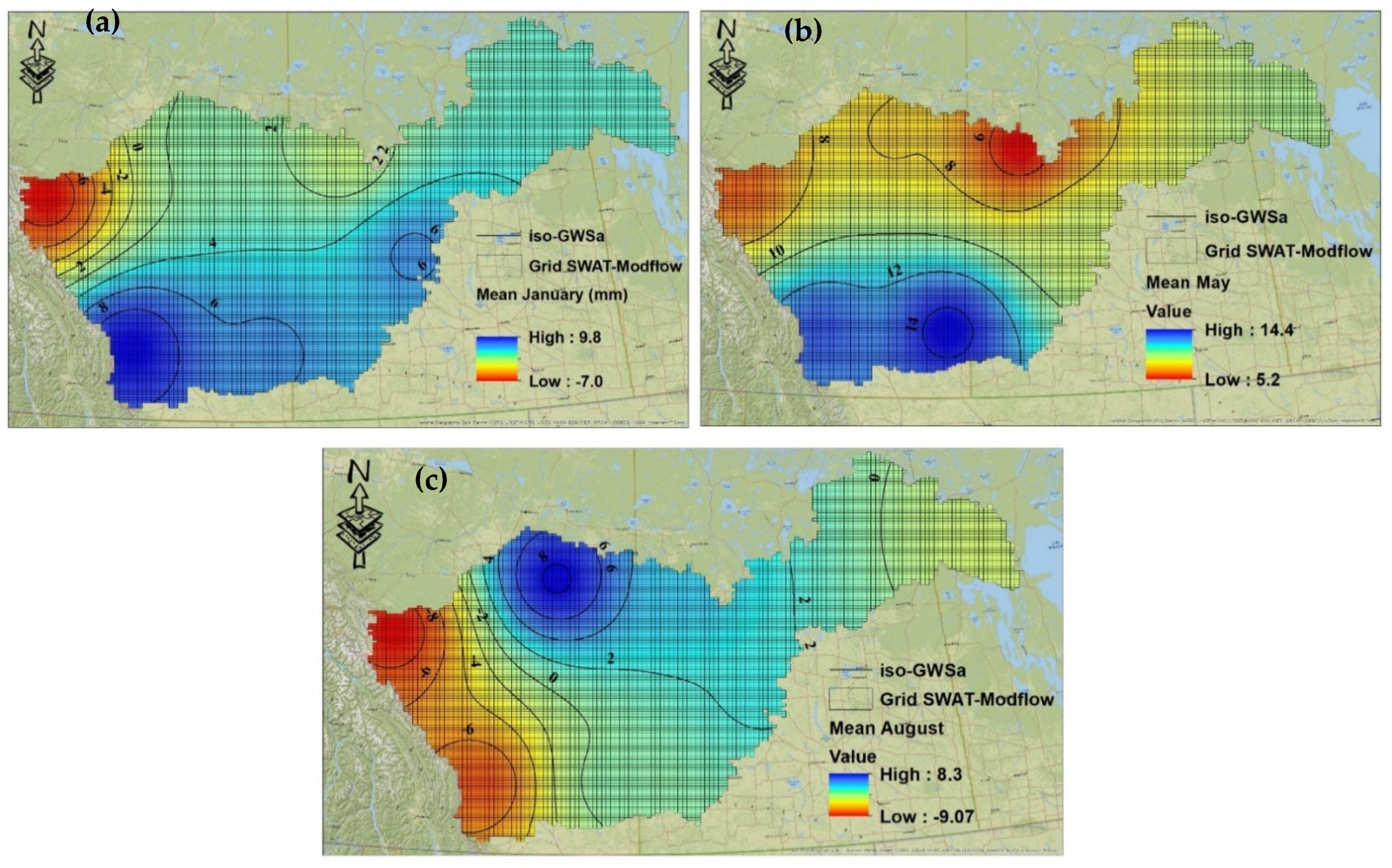
Figure 10 presents the spatial variability in groundwater storage that was derived from the GRACE/GRACE-FO data for January, May, and August.

During January, which is the peak of winter in the Canadian prairies, we observe negative GWS values across all ZBs, reflecting the freezing of surface water and almost zero recharge (Figure 10a). This is particularly notable in ZB4, which includes GWS values as low as −60 mm. At this time, farmers in the region may rely heavily upon groundwater extraction for agricultural purposes, including bovine breeding.

In May (Figure 10b), which marks the end of the snowmelt, positive GWS values are observed across all ZBs, with the highest values in ZB2 and ZB3. This response can be attributed to water from snow thaw, soil moisture, and canopy water, all of which contribute to increased recharge of the groundwater.

During August (Figure 10c), which is a transitional period between late summer and early autumn, negative GWS values become increasingly pronounced in most areas, again indicating that groundwater is being heavily exploited. This is particularly evident in ZB2 and ZB3, which experience intense groundwater extraction for irrigation during the summer growing season. ZB5, which is under pressure from surface water usage, also shows negative GWS values during this period. These findings highlight the need for sustainable water management practices that would ensure the long-term availability of groundwater resources in the Canadian prairies.

In Figure 10b, the positive values of GWS variations (between +5.2 mm and 14.4 mm) during the month of August show the potential of natural recharge in the filling of renewable reserves. Yet, this map also shows that in the study area, the recharge is difficult to locate, and infiltration is the main source of recharge:

• – Infiltration occurs directly on the outcrops in the mountainous regions. This recharge depends upon the physical conditions of the soil, and the intensity and duration of rainfall and snowmelt. This zone constitutes a fractured zone, which favours direct recharge of aquifers [41].
• – Infiltration of runoff water in ZB2 and ZB3, along rivers and aquifer boundaries that are even more complex in their hydraulic mechanisms, is considered only through their volume contributions to aquifer recharge. This infiltration is favoured not only by the deceleration of river velocity due to the flat topography in these two regions, but also by the hydraulic infrastructure of water exploitation.

5.3. Groundwater Depletion Estimation

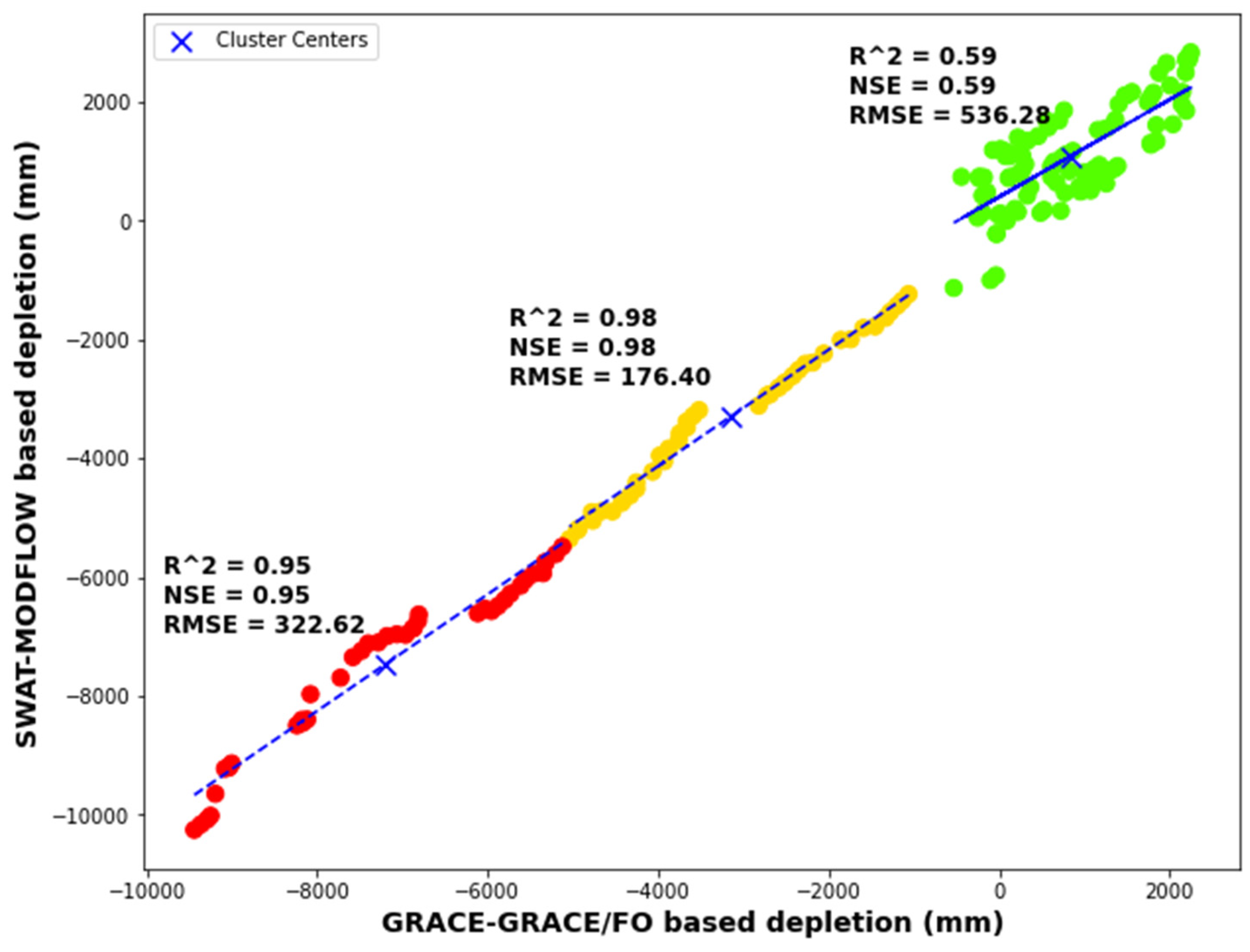
The approach that was used to estimate groundwater depletion is described in Section 4.3. Based on the GWS and GPLa comparison results, groundwater depletion was calculated using the coupled SWAT-MODFLOW hydrodynamic model and the GRACE-GRACE/FO data. The results show substantial agreement between the two methods (Figure 10). The significant finding of this analysis was the substantial agreement observed between the two methods. Figure 11 visually illustrates this agreement, underscoring the reliability and consistency of the coupled SWAT-MODFLOW hydrodynamic model and the GRACE-GRACE/FO data in estimating groundwater depletion. Between −10 m and −5.5 m (R2 ≈ 0.95): In this range, there is a strong positive correlation (as indicated by the high R2 value) between the GPLa and GRACE-based depletion calculations. This suggests that the two methods closely agree and provide consistent estimations of groundwater depletion within this depth interval. The high R² value of approximately 0.95 indicates that the relationship between the datasets is robust and can be described by a linear model with a high degree of accuracy.

Between −5.5 m and −2 m (R² ≈ 0.98): Within this range, the correlation is even stronger, with an R2 value of around 0.98. This signifies an excellent agreement between the GPLa and GRACE-based calculations, indicating that the two methods are highly consistent in estimating groundwater depletion in this depth interval. The relationship between the datasets is very close to a perfect linear fit, further enhancing confidence in the accuracy of the depletion estimates.

Between 0 and 3 m (R² ≈ 0.59): In this range, the R² value drops to approximately 0.59. While there is still a positive correlation between the GPLa and GRACE-based depletion calculations, it is weaker compared to the previous two intervals. This suggests that the two methods provide somewhat divergent estimations of groundwater depletion in this specific depth range.

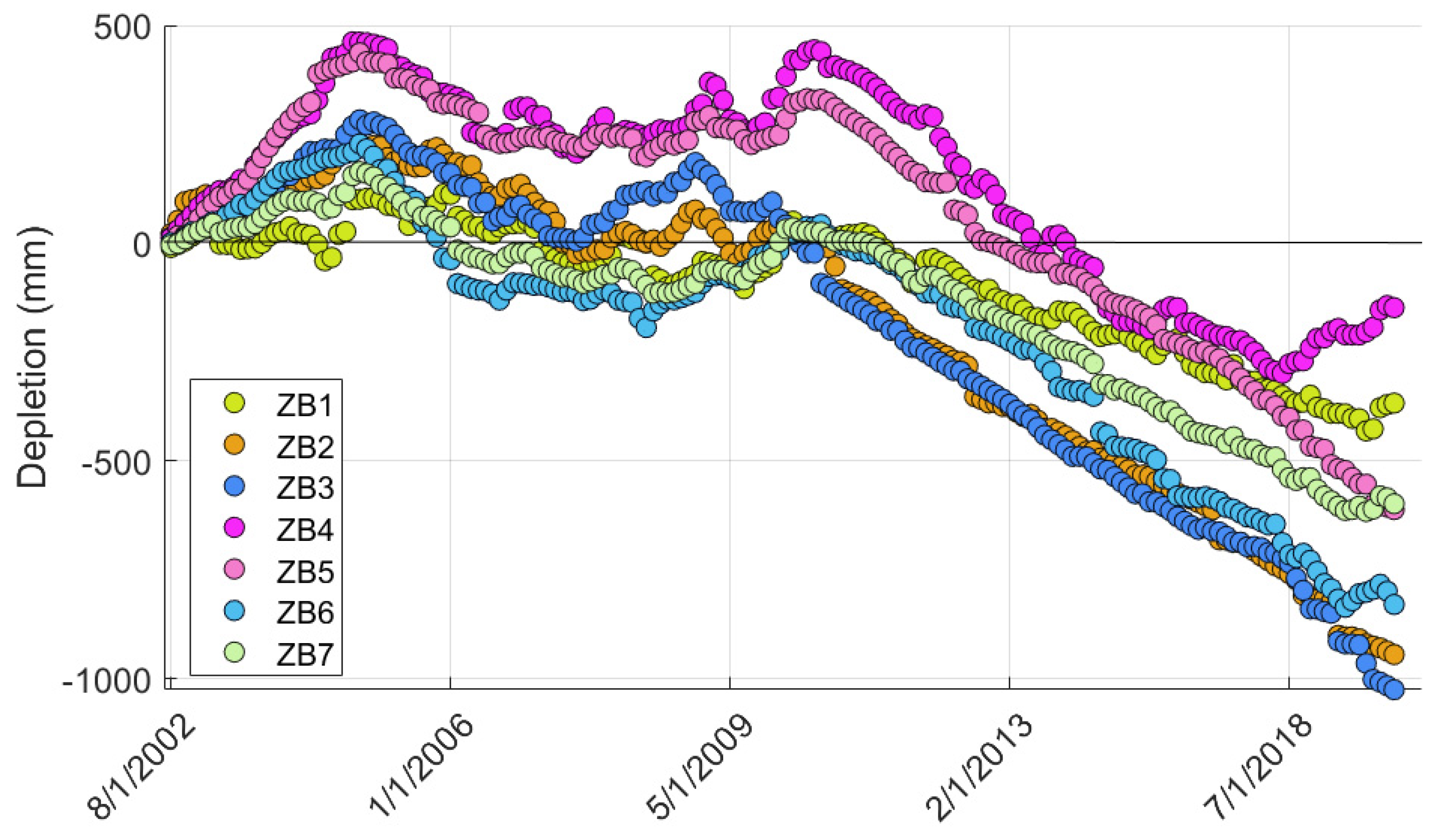
Figure 12 shows the cumulative depletion of the SRB aquifer system for ZB1 to ZB7. In this figure, positive values of depletion are considered as a refill of reserves due to diffuse recharge, and negative values represent an alternative over-exploitation of groundwater resources. Overall, the cumulative depletion of the SRB aquifer system shows two important phases: a recharge/exploitation phase (from 2002 to 2011); and an over-exploitation phase (from 2011 to 2019).

During the first phase, recharge is substantial for budget zone 4 and 5. An average of +0.35 m was added to the groundwater reserves in the period 2002–2011. This is mainly related to the fact that rainfall is higher in the northern SRB. Recharge is less pronounced in ZB1 and ZB7. The recharge peaks are observed during the months of April and May of each year and do not exceed +0.23 m for ZB1. Moreover, an increasing trend of depletion is observed in ZB2 and ZB3. In these areas, the minimal recharge of the aquifers shows small upwelling that does not even reach +0.19 m, on average. This shows the adverse effects of water exploitation on agriculture.

For phase 2, a generalized downward trend is observed. All the ZBs show a significant depletion, with a recorded maximum of −1 m for ZB3. The exploitation of groundwater in this area remains an important issue as many communities and industries depend on groundwater for their water needs. In fact, groundwater in this area is an essential source for crop irrigation, drinking water supply, mining, and power generation. For the same phase, the impact of the exploitation strategy is moderate: the maximum depletion values (up to −1 m) are observed at the water catchment area (agricultural and industrial zone) and at the boundary between the two provinces Alberta and Saskatchewan. This appears to be due to reduced recharge from SWE and exchange between deeper aquifers by both vertical drainage and horizontal percolation. These depletions quickly reached −1 m over the entire SRB after a short period from 2011 to 2018. The resulting depletions appear to be more or less down gradient more pronounced in the following years but with a more generalized spatial distribution over the central part of the SRB. However, these depletions are highly variable from year to year and very sensitive to variations in direct recharge.

In reality, aquifer recharge can decrease despite increased liquid precipitation in the SRB [42] for several reasons. Possible explanations include: (i) evapotranspiration can reduce the amount of water that seeps into the soil to reach aquifers; and (ii) the amount of water stored in the aquifer decreases, resulting from excessive extraction when water is pumped from an aquifer faster than it can be replaced by natural recharge. This can occur when water demand is high, such as in areas with high agricultural or industrial use. Finally, (iii) temperature augmentation can decrease recharge. Indeed, models indicate that climate change may result not only in an increase in the intensity of precipitation but also in an increase in the frequency of droughts [43]. If precipitation occurs as heavy downpours that are not absorbed by the soil, aquifer recharge may be reduced. In summary, reduced aquifer recharge can be due to a combination of factors, including natural factors such as evapotranspiration and climate change, as well as anthropogenic factors such as urbanization and excessive water extraction.

6. Discussion

Process-oriented methods like SWAT-MODFLOW can be used to assess the impacts of human activities on groundwater resources and to inform sustainable groundwater management decisions [18,43,44]. However, as with any model, results must be interpreted with caution and validated with field data and other sources of information to ensure accuracy [45,46]. In fact, process-oriented methods are modelling methods that aim to represent the physical processes involved in groundwater depletion. These methods use mathematical equations to simulate the flow of water in aquifers and interactions with other components of the hydrologic system, such as rivers, lakes, and precipitation [18,34]. For the case of SRB, the SWAT-MODFLOW coupled model is used as a process-oriented method.

This method demonstrated its usefulness for estimating surface water-groundwater interactions and depletion estimation, but it also has some limitations. The input data uncertainty is the most important limitation. Indeed, the SWAT-MODFLOW model requires accurate hydrologic data to calculate depletion, including aquifer permeability, hydraulic conductivity, and groundwater recharge. Yet, one of the key advantages of using SWAT-MODFLOW is that it allows the modelling of water dynamics in a watershed in an integrated manner, considering both surface and subsurface flows. This allows for a better understanding of the complex interactions between the two systems and a more accurate assessment of available water resources. In addition, SWAT-MODFLOW is a robust and well-established model that has been widely used in many studies for water management, environmental impact assessment, land use planning, and more. In summary, choosing SWAT-MODFLOW to model water dynamics in the SRB was an attractive option because of its ability to model surface and groundwater flows in an integrated manner, as well as its robustness and reliability as a groundwater and surface water simulation model.

The most important challenge in the study was data consistency. Model coupling also requires careful data management, ensuring that input and output data are compatible between the two models. Errors in the data can lead to erroneous results and biased predictions. Uncertainty in these data can affect the accuracy of the depletion calculation results. Furthermore, geographic limitations are important. The coupled SWAT-MODFLOW model may have geographic limitations in its ability to estimate groundwater depletion, particularly in areas with complex geology and heterogeneous aquifers like the SRB. Finally, the model requires significant resources for data collection, model calibration, and running simulations, which can be costly and require specialized technical expertise.

Despite these limitations, the coupled SWAT-MODFLOW model remains a useful tool for estimating depletion and understanding surface water-groundwater interactions. It is important to consider the limitations of the model when interpreting the results and to compare them to other sources of information to validate the conclusions.

From another perspective, satellite data-oriented methods (or remote sensing methods) are techniques that are used to obtain information about the Earth’s surface using satellite images [47]. These methods are used in many fields, such as agriculture, forestry, geology, meteorology, environmental monitoring, and natural resource management. Satellite data-driven methods can be used to calculate groundwater depletion by measuring changes in the ground surface [48,49,50]. Groundwater depletion occurs when the pressure exerted by groundwater pumping exceeds the recharge capacity of the water table, resulting in a drop in the water table.

GRACE and GRACE-FO data are satellite data that can be used to calculate water table depletion. Our second specific objective was to calculate GWS and depletion using this mission. These data have shown good accuracy in detecting changes in groundwater storage and in calculating groundwater depletion. Gravitational field variations measured by the GRACE and GRACE-FO satellites are correlated with changes in the amount of water in the groundwater table and demonstrate a good correlation with the observed data GPLa. For the case of SRB, these data can therefore provide information on groundwater level changes over large areas, including areas where field measurements are difficult or impossible. Their usefulness in tracking long-term trends in groundwater depletion in areas of high groundwater pumping and low groundwater recharge was impressive. These data can also help water managers identify areas where water resources are under pressure and where action needs to be taken to preserve them. For example, the study of (REF) introduces a parametric reservoir operation model, enhancing hydrological models’ accuracy. Two parameterization strategies are proposed, improving simulation accuracy in regulated basins, and offering versatility for widespread application. This study addresses the crucial influence of reservoirs on watershed systems by introducing a parametric reservoir operation model. It emphasizes the need for accurate representation of reservoir effects, which significantly impact streamflow magnitude and timing. The model based on piecewise-linear relationships between reservoir storage, inflow, and release, aims to approximate real reservoir operations.

Although this method was widely used to calculate GWS and has provided accurate results, it also has limitations. The most important limitation is the spatial coverage, which is relatively low and may limit its ability to detect local changes in groundwater depletion.

The second limitation is the measurement of total depletion: GRACE/GRACE-FO measures total groundwater depletion, which can include both anthropogenic factors (such as excessive groundwater use) and natural factors (such as climate variations). Therefore, it can be difficult to distinguish between human and natural effects on groundwater depletion. We cannot forget the validation of results. In fact, GRACE/GRACE-FO results need to be validated in the field by other measurement methods, such as water level measurements in wells. This validation may be difficult in areas where monitoring data are sparse.

The state of groundwater depletion in the SRB could be assessed using both methods (SWAT-MODFLOW and GRACE/GRACE-FO data). The comparison between these methods shows good agreement. Both methods show that the depletion in the SRB can reach 1 m in some areas. This may be due to the combined action of climate change and overexploitation, particularly in areas where intensive agriculture and mining are practiced (ZB2 and ZB3). Industrial activities, including gas extraction and hydraulic fracturing, use also an important amount of water, with a consequence on groundwater. Prolonged droughts can reduce precipitation and groundwater recharge, which can lead to lower groundwater levels, which can have serious consequences for ecosystems, economic activities, and communities that depend upon the resource.

7. Conclusions

In this study, a coupled SWAT-MODFLOW model and GRACE/GRACE-FO satellite gravimetry data were respectively used to estimate groundwater depletion in the SRB. According to the results that we obtained, the process-oriented coupled SWAT-MODFLOW model can simulate surface and subsurface flows and their interactions with accuracy. Depletions estimated by this model reach 1 m in some areas, such as central Alberta and Saskatchewan, revealing great pressure on groundwater resources in these regions. A quite similar result was found with satellite gravimetry data from GRACE/GRACE-FO. Both model and satellite-based approaches were used in this study, generating convincing performance metrics compared to those obtained for in situ piezometric data. These methods appear well adapted to elucidate the hydrodynamic functioning of aquifers at the scale of SRB. Future work will explore the use of artificial intelligence approaches to better estimate groundwater from satellite gravimetry and to facilitate their integration into coupled models. Moreover, anthropogenic activities in this basin, such as excessive groundwater pumping for irrigation, industrial use, or municipal water supply, can significantly affect groundwater levels. Over-extraction of groundwater can lead to the lowering of water tables, causing a decline in groundwater levels. Additionally, land-use changes associated with agriculture and urbanization can impact the recharge of aquifers, reducing the replenishment of groundwater resources. Effective management and regulation of anthropogenic impacts on groundwater are essential to maintain sustainable groundwater levels and preserve the region’s water resources.