Review

Dynamic Groundwater Contamination Vulnerability Assessment Techniques: A Systematic Review

1
Faculty of Engineering and Design, Atlantic Technological University, ATU Sligo, Ash Lane, Ballytivnan, F91 YW50 Sligo, Ireland
2
Department of Building & Civil Engineering, Atlantic Technological University, Dublin Road, H91 T8NW Galway, Ireland
3
School of Engineering, Trinity College Dublin, College Green, D02 PN40 Dublin, Ireland
*
Author to whom correspondence should be addressed.
Hydrology 2023, 10(9), 182; https://doi.org/10.3390/hydrology10090182
Submission received: 11 July 2023 / Revised: 10 August 2023 / Accepted: 18 August 2023 / Published: 4 September 2023
(This article belongs to the Section Hydrological and Hydrodynamic Processes and Modelling)

Abstract

:
Assuring the quantity and quality of groundwater resources is essential for the well-being of human and ecological health, society, and the economy. For the last few decades, groundwater vulnerability modeling techniques have become essential for groundwater protection and management. Groundwater contamination is highly dynamic due to its dependency on recharge, which is a function of time-dependent parameters such as precipitation and evapotranspiration. Therefore, it is necessary to consider the time-series analysis in the “approximation” process to model the dynamic vulnerability of groundwater contamination. This systematic literature review (SLR) aims to critically review the methods used to evaluate the spatiotemporal assessment of groundwater vulnerability. The PRISMA method was employed to search web platforms and refine the collected research articles by applying certain inclusion and exclusion criteria. Despite the enormous growth in this field in recent years, spatiotemporal variations in precipitation and evapotranspiration were not considered considerably. Groundwater contamination vulnerability assessment needs to integrate the multicriteria decision support tools for better analysis of the subsurface flow, residence time, and groundwater recharge. Holistic approaches need to be formulated to evaluate the groundwater contamination in changing climatic scenarios and uncertainties, which can provide knowledge and tools with which to prepare sustainable groundwater management strategies.

1. Introduction

Groundwater is an essential source of fresh water, supplying water for agricultural, domestic, and industrial demand. It also supports the various needs of the ecosystems across the world. Groundwater makes up the world’s largest freshwater reservoir, accounting for 99% of the liquid freshwater stock on Earth [1]. According to a recent report by the United Nations, groundwater comprises almost half of the world’s drinking water, around 40% of the water used for irrigation, and one-third of the water sup-ply required for industry [2]. This vital source of life has become a significant concern in the last few decades because of its scarcity and vulnerability to pollution. Enormous research studies have been conducted to quantify this vital issue [1,3,4,5,6,7,8,9,10]. Increasing water usage to meet the demands of an increasing population has led to significant groundwater depletion in populated urban and rural areas due to agricultural land use. In many regions, aquifers have become susceptible to either complete or seasonal exhaustion [1]. The groundwater contamination vulnerability has also been increasing due to anthropogenic practices and geogenic involvement.
Water naturally contains several different dissolved inorganic constituents such as calcium, magnesium, sodium, potassium, chloride, sulfate, carbonate, etc. In addition, minor constituents may be present in the water, such as iron, manganese, fluoride, nitrate, and strontium. It may also contain trace elements, such as arsenic, lead, cadmium, and chromium, in amounts of only a few micrograms per liter. The presence of these constituents or elements is dependent on the Earth’s strata holding the water. They are important from a water-quality perspective [11]. But when the natural occurrence elevates the concentration (acceptable for a specific purpose) of these elements, they harm human health and are called pollutants. As these contaminants originate from rock material by leaching or withering [12], this is called geogenic contamination. Geogenic contamination can be defined as a phenomenon caused by geologic process-es. Conversely, groundwater contamination is mainly a combination and sequence of surface and subsurface processes. These processes are directly involved in groundwater recharge. As the climate controls precipitation and evapotranspiration, climate change’s impact alters the progression of recharge by directly speeding up or delaying the surface and subsurface processes.
Contamination and pollution are not the same. The first is the presence of a sub-stance in an amount above the background concentration level. On the other hand, pollution is contamination that results in or can create adverse biological effects to the resident community. In this paper, we intend to combinedly discuss the spatiotemporal aspects of the groundwater contamination and groundwater pollution. Deeper aquifers may be less affected by biological and chemical substances; however, contamination of shallow groundwater sources has become endemic due to human interference with the near-surface or subsurface water flow pathways. Agricultural fertilizers, pesticides, solvents, and chemicals are used in the manufacturing industries, mining, energy production, commercial applications, and pharmaceuticals industry, and human waste-induced pathogens lead to chronic contamination of shallow and deep ground-water worldwide [1]. On a regional scale, groundwater can also be contaminated by geogenic factors (naturally occurring elevated concentrations of certain elements) through adsorption/desorption kinetics associated with soil or rock minerals such as arsenic and fluoride [1]. In addition, groundwater quality is also susceptible to various climate change effects, such as changing precipitation patterns, increasing evapotranspiration (ET), etc.
Pesticides’ fates and transport in the subsurface under agricultural land use are sensitive to climate change-induced changes in rainfall seasonality and intensity, as well as changed rates of recharge [13,14]. Furthermore, climate change and increasing global urbanization may also increase the risk of flooding. This urban flooding increases the loading of common urban pollutants like oil, solvents, and sewage into groundwater [15,16]. In short, the groundwater system is continuously changing due to its dynamic interactions with physical and socio-economic systems. The observed or expected groundwater state changes often diverge from what is most desirable, and it is far beyond the scope of a single individual to control these changes. Groundwater is a common pool resource but can cause significant discrepancies between the interests and preferences of individuals compared to those of a local community. These reasons motivate and justify increased studies and interventions in groundwater resource management [10].
“Vulnerability is not an absolute characteristic, but rather a relative, non-measurable, dimensionless property indicating where contamination is most likely to occur” [17]. The concept of aquifer vulnerability was introduced by [18]. It was defined as “the possibility of percolation and diffusion of contaminants from the surface into natural water table reservoirs, under natural conditions”. Ref. [19] described groundwater vulnerability as “an intrinsic property of a groundwater system that depends on the sensitivity of that system to human and/or natural impacts”. According to [20], the vulnerability of groundwater can be intrinsic or specific depending upon the nature of the contamination. Intrinsic vulnerability is a function of hydrogeological factors by which pollutants can reach and diffuse into groundwater when introduced to the surface [19]. Intrinsic vulnerability is sensitive to natural or geogenic contamination and does not consider anthropogenic activities [21]. Specific vulnerability refers to the susceptibility to a particular and/or a group of pollutants based on contaminant properties, attenuation processes, and transport characteristics [22,23]. Specific vulnerability refers to the impact of specific land use. In other words, this integrates the risk of the contaminants generated by human activities [17].
Ref. [23] described three main approaches with which to assess the qualitative vulnerability of groundwater. The first approach (knowledge-based) evaluates the vulnerability considering transport processes only in the unsaturated zones and ignores those in the saturated zones (e.g., aquifer media). The second approach (data-driven) considers groundwater flow and contaminant transport processes in the aquifer systems. This approach is based on the demarcation of regions to protect the wellheads for groundwater supply systems. The final (process-based) approach is based on a holistic method to assess the aquifer vulnerability, considering both surface and subsurface processes. Based on the above generic approaches (knowledge-based, data-driven, and process based) suggested by [23], groundwater vulnerability modeling techniques can broadly be classified into three categories (overlay and index-based models, statistical models, and process-based models). Models are computer-based programs which can represent an approximation of the field situations [24]. Based on the purpose of the study, groundwater models are generally used to predict space and time, interpret the system dynamics, and analyze the flow in a conceptual hydrogeological setting [24].
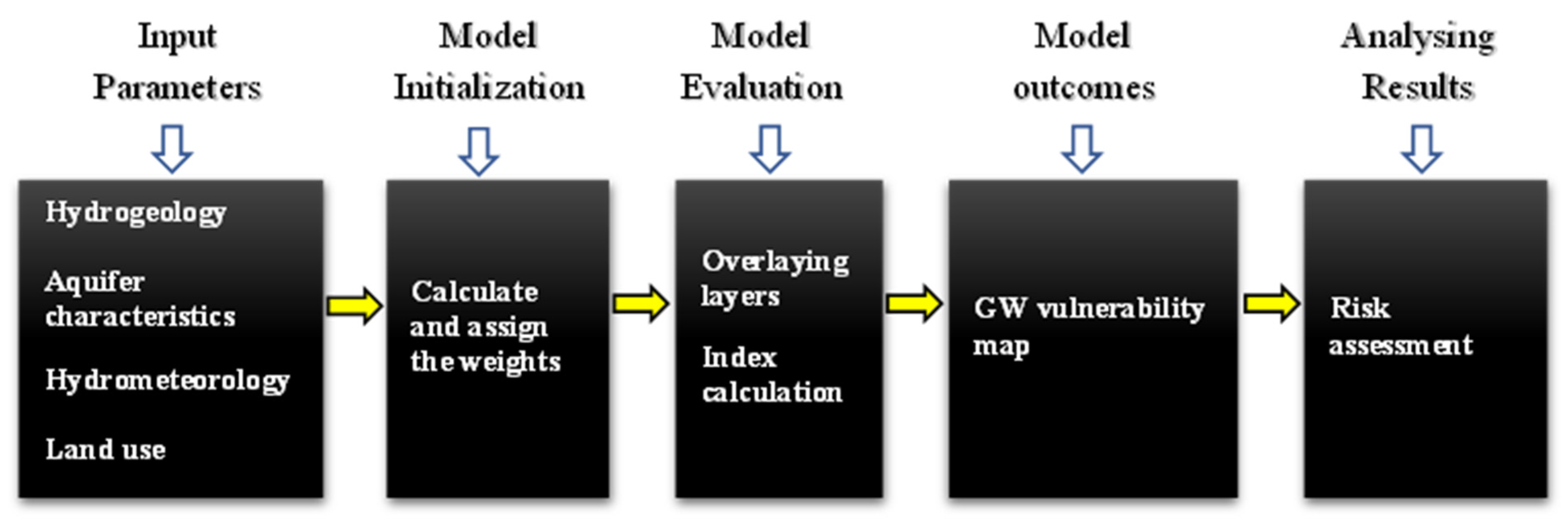
Overlay and index-based method (knowledge-based): These methods combine physiographic variables and assign them numerical ratings to map the physiographic and anthropogenic characteristics of the study area. Later, these numerical ratings are superimposed onto each other to develop a composite susceptibility index. These rating systems are equal or weighted depending upon the relative degree of their control in the entire assessment [25].
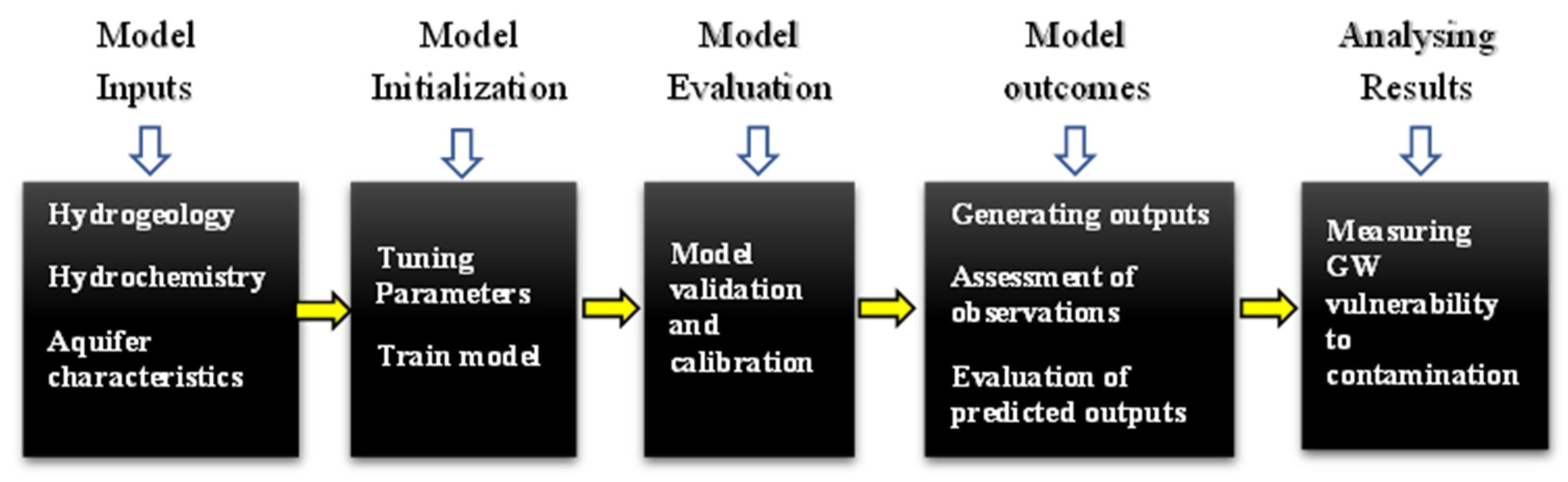
Statistical method (data-driven): These techniques combine contamination concentration, natural factors (e.g., recharge or surface and sub-surface processes), and a potential source of contamination, i.e., land use (e.g., pollution from agricultural fertilizer and septic tanks), to establish a relationship among them, which can quantify the groundwater’s vulnerability to contamination. These methods are based on the processes of map correlation and map integration. In the statistical methods, the known occurrence of the contamination (training points/response variables) is combined with spatial data (explanatory variables/predicting factors) to explain the relationship between each factor and the training points [26].
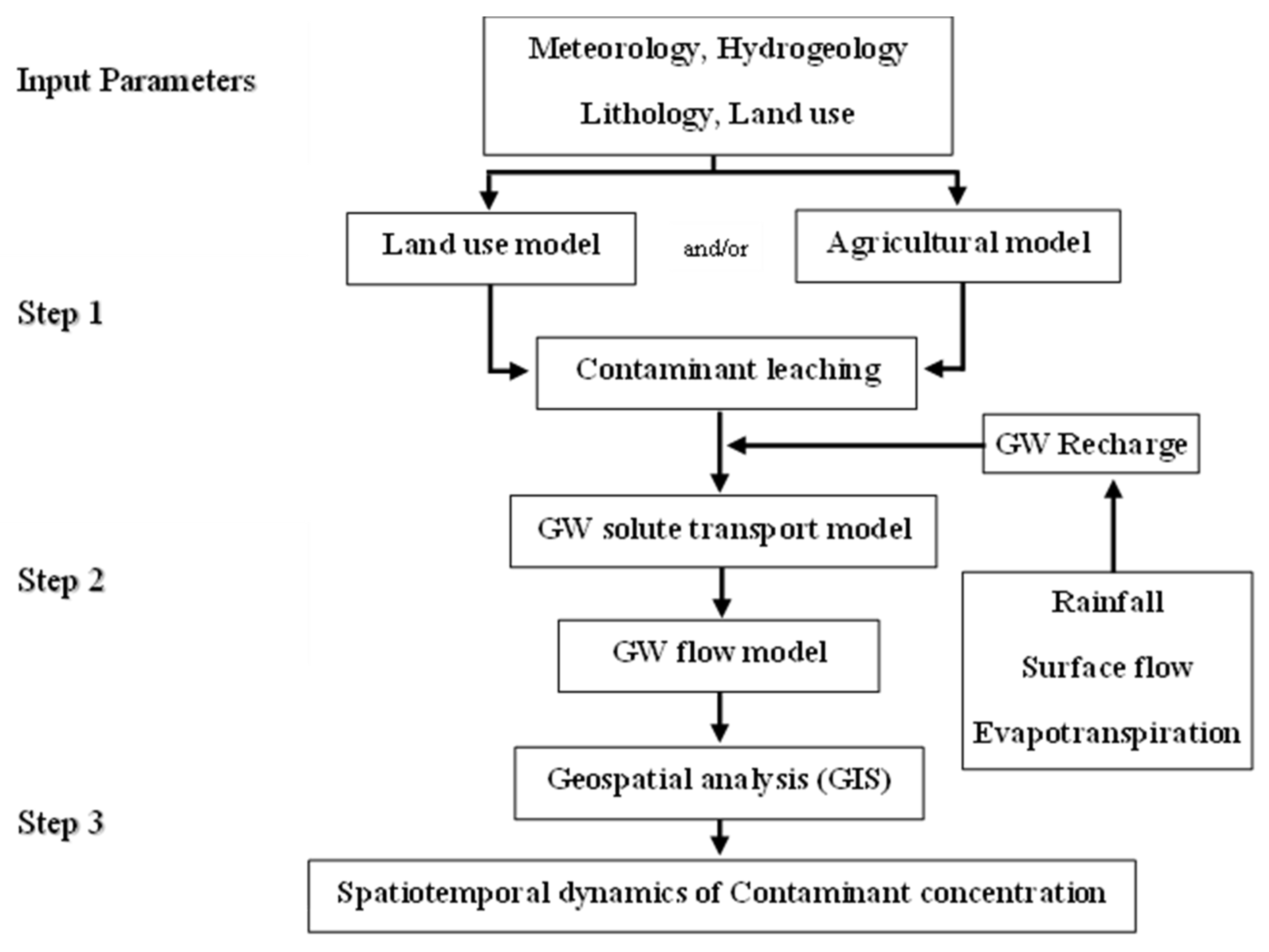
Process-based method (physical process-based): Process-based methods are based on a quantitative approach which employs mathematical simulations for the assessment of groundwater vulnerability. These methods are helpful in calculating the fate and transport of solutes, groundwater flow, and contaminant concentration in the vadose zone and/or aquifers. These approaches are also suitable for creating reference criteria which can be clearly identifiable. These reference criteria are required for the simulation and validation of the model [4]. These can predict the consequences of a proposed action which can be used for deciding on land-use policies.
The lists of widely used approaches (overlay and index-based, statistical, and process-based) are presented in Supplementary Materials S1.
Aside from the above classification, groundwater vulnerability assessment studies can be classified into two categories based on the purpose of the study, and these are “resource” protection or “source” protection. Resource protection is based on protecting the aquifer in order to safeguard the entire underlying groundwater body. It only considers vertical seepage in the unsaturated zone to the uppermost groundwater surface [4]. Source protection is based on protecting a spring or well from contamination by considering vertical seepage in the unsaturated as well as the lateral flow in the saturated zone [4,6].

Spatiotemporal Assessment of Groundwater Vulnerability

Traditionally, models of groundwater contamination were based on the “static” hypothesis that groundwater’s vulnerability to contamination is not time-dependent. However, groundwater’s vulnerability is inherently dependent on groundwater recharge, which is mainly controlled by precipitation and evapotranspiration as well as the surface- and subsurface-level structure of the ground. Therefore, groundwater recharge is highly time-dependent, and strategies for evaluating future groundwater vulnerability in a changing climate and land-use scenarios must consider the “dynamic” concept of vulnerability [21]. Most environmental processes depend on space and time, with time series and spatial data series being strongly reliant on each other. According to the deterministic theory of spatiotemporal hydrogeological variability, a time series is a systematic pattern that helps to identify the trend/periodic factor/shift and/or the combination thereof [27,28] first introduced the concept of spatiotemporal vulnerability in hydrology. It was defined as “the ability of this system to cope with external, natural and anthropogenic impacts that affect its state and character in time and space”. The application of spatiotemporal analysis became a part of groundwater vulnerability assessment during the last three decades, along with the significant development of quantitative applications in the hydrological domain. Studies have shown that spatiotemporal assessment has evolved as a powerful tool for investigating hydrologic/hydrogeologic time series data for surface and subsurface flows. The time dependency of groundwater’s vulnerability to contamination is already well defined, and many researchers have conducted several studies to analyze groundwater’s temporal vulnerability using various qualitative and quantitative approaches.
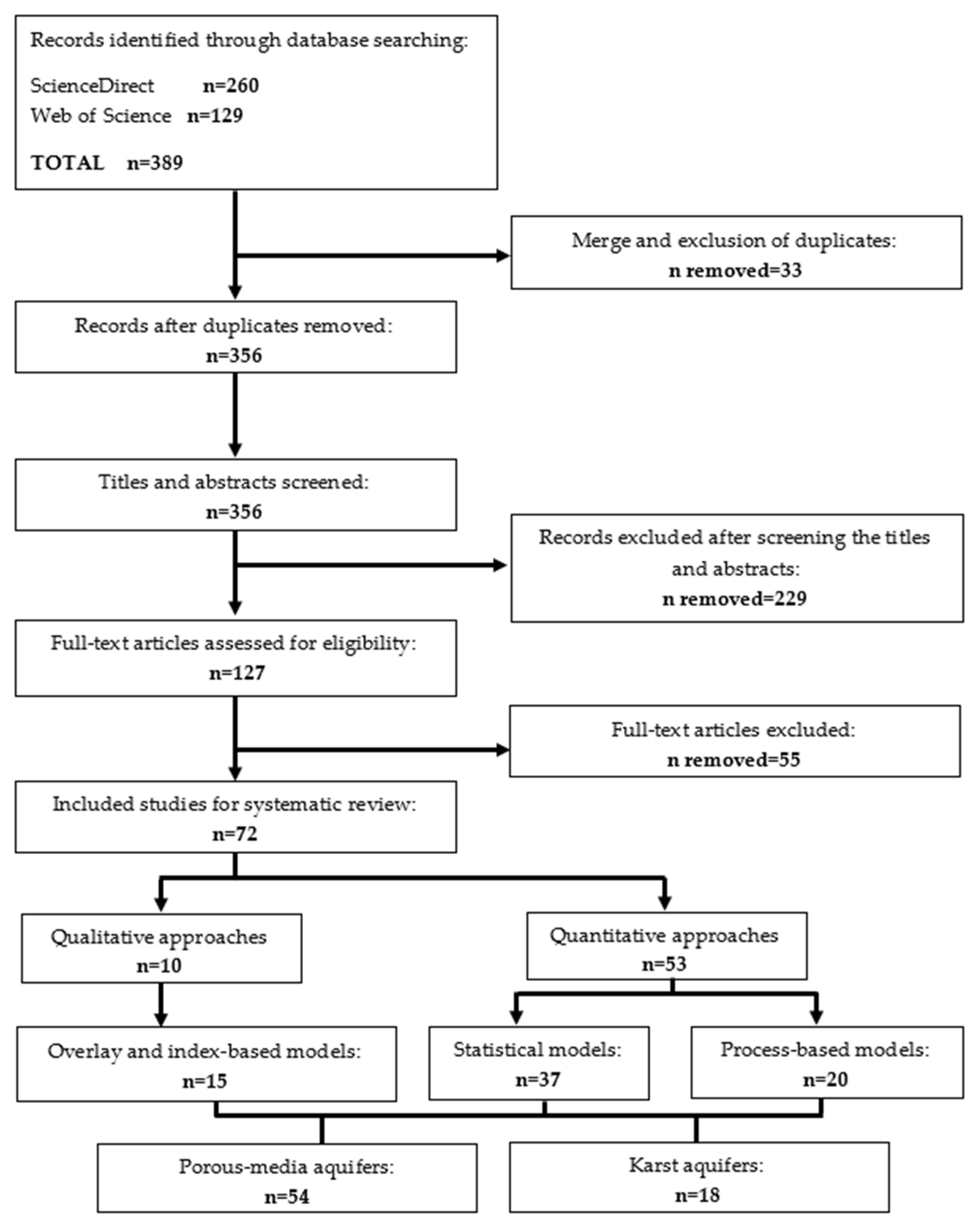
This review paper aims to evaluate the recent developments in spatiotemporal assessment techniques for groundwater contamination. Although, in recent years, many reviews have demonstrated the trend in modeling techniques for groundwater vulnerability assessment [4,5,29,30], a comprehensive review showing the application of a potential temporal analysis of groundwater vulnerability is lacking. This paper systematically reviews recent advancements in dynamic vulnerability of groundwater contamination and highlights the research gaps in terms of simulating the models and setting up the time-dependent drivers. This article only reviewed studies which mainly evaluated the chemical substances released from anthropogenic activities and geogenic processes. Studies on bacteriological pollution were not included in this paper as they are out of the scope of this review. In the future, a separate review article can be presented concentrating only on bacteriological pollution.

2. Methodology

The review process employed the guidelines of Preferred Reporting Items for Systematic Reviews and Meta-Analyses/PRISMA [31] to identify the state of knowledge of dynamic groundwater contamination vulnerability models. A systematic review of published studies on spatiotemporal vulnerability assessment for groundwater contamination was carried out. PRISMA provides a reliable structure with which to assess the existing research articles and to define the inclusion and exclusion criteria. PRISMA follows four main steps. The first is identifying the data sources and limiting the search criteria, then including or excluding the sample according to set standards based on the purpose of the review. Third is extracting the data of interest from the final selection. Finally, the findings are analyzed and summarized. We are aware that all relevant articles may not have been included in the review. However, a significant number were extracted through our PRISMA search. In some cases, particular references were included for discussion despite not being included in the review process. The PRISMA flow diagram is presented in Figure 1.
The literature search was conducted using Web of Science (WoS) and ScienceDirect (SD). Articles published in groundwater- and environmental management-related journals listed in Science Citation Index Expanded (SCIE) were considered for this review. The search procedure was divided into two segments: one for porous media aquifers (2010–2021) and one for karst aquifers (2000–2021). The literature search was performed in WoS and SD using the Boolean operators AND, OR, and NOT. The details of the search criteria can be found in Supplementary Materials S2.
Inclusion and exclusion criteria were imposed at three different stages. Title and keywords: studies must have been conducted to assess the groundwater contamination vulnerability (i.e., exclusion of surface water pollution, soil pollution, forest and wetland pollution, watershed dynamics and catchment management, riverbank morphology, and filtration). Abstract: the research must have modeled the spatiotemporal dynamics of groundwater contamination vulnerability only for inland aquifers (i.e., exclusion of groundwater management and remediation, human health, coastal aquifers, and groundwater salinity). Full text: the research studies must have used modeling techniques to analyze and predict the regional-scale contamination vulnerability, not only the qualitative explanation of observed spatiotemporal data. In the above procedure, when adequate information was not present to exclude an article in the first stage, it was included in the next step and so forth until full-text assessment was conducted. The details of the search criteria can be found in Supplementary Material S2. Finally, 72 articles were selected through full-text examination for this systematic literature review.

3. Results and Discussion

This systematic literature review separated the porous media aquifers from the karst aquifers, then reviewed the dynamic vulnerability assessment techniques. This will be described in two different sections, below.

3.1. Porous Aquifer Vulnerability Assessment

3.1.1. Overlay and Index-Based Models

Overlay and index-based models are mainly subjective/knowledge-based methods. These are the oldest groundwater contamination modeling techniques. The execution of these methods is easy and demands minimal parameters to assess groundwater vulnerability (Figure 2). The index-based models employed in the last decade for the assessment of dynamic groundwater vulnerability assessment are IEA-UEF [32], WQI [33], m-HPI [34], GOD [35], Pesticide DRASTIC [36], DRASTIC [37], GWV [38,39], and NPI [40].
This review identified that two revolutionary indices (DRASTIC and GOD) are still popular among researchers who employ index-based analysis in their spatiotemporal vulnerability studies. However, these have been modified and/or integrated according to the needs of the studies. Ref. [36] integrated statistical analysis, such as hierarchical cluster analyses (HCA), and discriminant analysis to establish the relationships between the locations and to determine the seasonal effect, respectively. Ref. [37] integrated the analytical hierarchy process (AHP) theory with DRASTIC to modify the weightings and ratings based on the experience and knowledge of specialists or users. AHP was also incorporated by [35] using the GOD modeling technique. As GOD is a static model, the assessment of the spatiotemporal variations was computed using ANOVA. During the last decade, besides vulnerability, many spatiotemporal groundwater quality assessments have studied water quality index (WQI), the immune evolutionary algorithm–universal exponential formula (IEA-UEF), modified heavy metal pollution index (m-HPI), and nitrate pollution index (NPI). The WQI [33] and an updated and integrated version of the WQI called the IEA-UEF [32] assessed the groundwater quality samples collected for a certain period to investigate the contaminants influencing the groundwater quality and/or to specify the groundwater quality zones. Two new approaches, m-HPI [34] and NPI [40], were introduced in order to analyze the spatiotemporal trend of heavy metal and nitrate, respectively, based on the collected groundwater samples for a given period. These models (WQI, IEA-UEF, m-HPI, and NPI) employed kriging and/or inverse distance weighting (IDW) method to fulfill the need for spatial trend analysis. All of these models are suitable for groundwater quality assessment. Understanding the groundwater quality status and tracking the pollution trend is crucial. However, these trends are meaningless when not incorporated with the physico-hydrological parameters. It is essential to know the geogenic or anthropogenic history of the aquifer systems and the geophysical processes to draw meaningful conclusions regarding the analysis and policy making. Therefore, these models are lacking in terms of defining the dynamic groundwater vulnerability. Refs. [38,39] presented a long-term predictive model. They predicted the groundwater vulnerability for three periods: past (1961–1990), present (2011–2040), and future (2041–2070). They employed the groundwater vulnerability (GWV) method to assess and predict the long-term vulnerability. This method uses various important climatic parameters to evaluate and predict the groundwater vulnerability scenario while considering climate change. A summary of the index-based groundwater vulnerability assessment models reviewed in this paper is presented in Table 1.

3.1.2. Statistical Models

Statistical models are based on data-driven methods, ranging from conditional probability analysis and regression to descriptive statistics. Statistical involvement allows objective methods to determine the relationship between the level of contamination and predictor factors. Over the last decade, many attempts have been initiated to calculate groundwater’s vulnerability to contamination using statistical modeling techniques (Figure 3).
Previously, many reviews accumulated these models and presented detailed critical reviews [4,5,30]. This review was conducted only to evaluate the time series statistical analysis developed in the last decade for groundwater vulnerability analysis. These models are classified into the following categories: (i) spatial interpolations, (ii) multivariate statistics, (iii) spatial autocorrelations, (iv) artificial intelligence, (v) regressions, (vi) Bayesian networks, (vii) decision trees, (viii) probabilistic methods, and (x) cluster analysis.

Spatial Interpolations

In groundwater vulnerability assessment, spatial interpolation uses information on sample location points to predict and map the unsampled locations. Depending on their probabilistic nature, spatial interpolation techniques can be divided into deterministic (e.g., IDW) and geostatistical (e.g., Kriging) approaches. This review found that kriging was the most often used for groundwater vulnerability estimation. Ref. [41] employed disjunctive kriging (DK), along with ordinary kriging and cokriging, to assess the probability of non-point source groundwater contamination under the influence of agricultural land use. They collected groundwater samples according to the summer crop cycle from 2004 to 2006. The results indicate that interannual climate variation and fertilization control nitrate contamination. Therefore, from an agri-environmental perspective, this method can achieve a reliable outcome for the decision-makers. Ref. [42] employed ordinary point kriging to assess the spatiotemporal groundwater contamination in the Mediterranean region. They monitored the groundwater table depth and contours, pH, EC, and NO3 during the pre-monsoon (June) and post-monsoon (October) seasons in 2009 and 2010 from 220 monitoring wells. The outcome reported how rainfall patterns can change the evapotranspiration pattern, which controls the amount of NO3 leaching (higher temperature and lower relative humidity can increase evapotranspiration and minimize the risk of NO3 leaching).
Ref. [43] proposed a common decision framework combining monitoring data and ordinary block kriging-based modeling simulation to investigate the vulnerability of groundwater pesticides. Water samples were collected from 2005 to 2009 to analyze five plant protection products (PPPs), such as terbuthylazine (Tba), glyphosate (Gly), pendimethalin (Pend), s-metolachlor (s-Met), and chlorpyriphos (Cpyr), as well as a terbuthylazine metabolite called desethyl-terbuthylazine (d-Tba). This approach combines spatial modeling of environmental fate and long-term monitoring information on the occurrence of PPPs in wells. The VULPES system [44] was employed for modeling purposes. VULPES helped to identify the potential pesticide vulnerability zones on a territorial scale, and monitoring provided the known occurrences of contamination. This dual characteristic of a single model provides policymakers with a more reliable set of information with which to decide on pesticide use, creating guidelines and directions for further investigation.
Ref. [45] presented a groundwater nitrate vulnerability assessment for an arid or semiarid region. Water quality data on nitrate concentration were sampled (Na, Cl, SO4, and NO3) from 2000 to 2013. To understand the spatial distribution of the concentration and the temporal extent of the distribution, an ANOVA-based (analysis of variance) method, least significant difference (LSD), and ordinary kriging (OK) were employed. In addition, a coefficient of variation dimensionless index was fitted to compare the NO3 variations in pollution plumes. The outcome resulted in a significant explanation of the relationship between nitrate concentration, sediments, and hydrogeological situations. The high permeability of coarse-grained sediments reduced the residence time of the contaminants in unsaturated zones, and the nitrate was able to reach the groundwater quickly with the help of vertical streams.
Similarly, Refs. [46,47] also used OK to assess the spatiotemporal variation of fluoride and nitrogen concentrations, respectively. In addition, Ref. [46] used PCA and Varimax Rotation to identify the significant and derive the factors. Seasonal variability in fluoride concentration can be seen due to weathering from carbonate minerals. Ref. [48] employed OK to assess the dynamics of nitrate concentration. Water samples were collected from July 2018 to September 2019, and the analysis was conducted by dividing the samples into four seasons, i.e., fall (September–November), winter (December–February), spring (March–May), and summer (June–August), to identify the seasonal variability.
Ref. [49] integrated OK and IK to estimate the spatio-seasonal distribution of nitrate concentration and to create a zonation map of the distribution. Groundwater samples were collected during the summer (July 2012 and September 2012) and winter (April 2012 and March 2013). Later, a semivariogram was fitted to identify the spatial dependency of nitrate values. Ref. [50] conducted a study to map the seasonal and annual GW arsenic contamination. Two interpolation methods, Thiessen polygon and OK, as well as a regression model were integrated to map the arsenic concentration and predict the future trend using time series data. Arsenic concentration samples were collected before and after the monsoon seasons from 2006 to 2008. An evident seasonal fluctuation was found with a high concentration in post-monsoon seasons due to the leaching of arsenic from soil lattices (where arsenic is present as arsenical ore), following the process of percolation of rainwater through soil grains. Ref. [51] employed the inverse distance weighted (IDW) method and PCA to investigate the pesticide concentration in groundwater.
Ref. [52] employed a semivariogram to assess the impacts of land-use change and agricultural activities on groundwater contamination. Water samples for nitrate concentration were collected in 2002 and 2007 to compare the water quality. A spherical isotropic model was fitted to the empirical semivariances. This method combined the spatially distributed variables and nitrate concentrations throughout the classified range. Cross-validation was conducted using kriging. Similarly, Ref. [53] investigated the nitrate input to the subsurface through GW recharge using variogram geostatistical analysis. Water samples from 13 streams were collected every two weeks from January 2010 to February 2011 to assess the discharge, EC, nitrate concentration, pH, and water temperature. Time series analysis of these parameters explained the relationships between different hydrological responses in a common rainfall regime.

Multivariate Statistics

In the past decade, many multivariate analyses were conducted to analyze the spatiotemporal distribution of contaminants in the groundwater. Principal component analysis (PCA) is one of the most significant and widely used parameter-identifying tools and data reduction techniques for almost all environmental studies. This literature review found that in the recent past, PCA integrated with factor analysis (FA), hierarchical cluster analysis (HCA), regressions, or spatial interpolation methods was intensively used in the vulnerability assessment of groundwater contamination. Ref. [54] presented a GIS-based study by combining PCA and IDW to investigate the nitrogen sources in groundwater under various land use scenarios. Ref. [55] combined PCA and FA to track the urban pollution source and the concentration level. FA was employed to reduce the involvement of less significant parameters within each component. This reduction procedure involved extracting a different set of varifactors by rotating the axes defined by the PCA extraction. A K-means-based cluster analysis (CA) was employed on the FA-extracted varifactors to analyze the similarities in the water quality. Ref. [56] employed PCA to track the source and transport of chlorate in the groundwater under agricultural land use. Ref. [57] investigated the spatiotemporal vulnerability of GW quality using a robust PCA (ROBPCA) method. To avoid the drawbacks of classical PCA (such as anomalous observations, overestimating the variance, etc.), they compared and proposed ROBPCA for the measurement of the seasonal and hydro-chemical characteristics of the aquifer. ROBPCA is a useful method for identifying spatiotemporal variations in GW quality when hydro-chemical processes are diverse and anomalous samples are available.
Ref. [58] quantified the trend of groundwater contamination by evaluating the spatiotemporal variations in the water quality parameters. They integrated a GIS-based groundwater quality index (GQI), HCA, and PCA to map the groundwater quality zones, identify the potential sources of contamination, investigate the process of geochemical change in GW quality, and identify the responsible factors, respectively. The Kriging interpolation technique was also fitted to demonstrate the spatial distribution of the specified significant principal components. Ref. [59] studied the fluoride concentration using FA. We already discussed that this approach is useful for replacing large matrices by introducing new variables. They created land use maps for the years of 2001–2003 (ETM+) and 2004–2008 (TM) using a supervised (maximum likelihood) method to understand the influence of paddy fields on groundwater fluoride concentration. A probability occurrence was calculated to identify the distribution of fluoride concentration with time. Ref. [60] employed FA and HCA to map the chemical variability in groundwater as well as their probable sources. FA is a two-dimensional approach which can analyze two-way datasets, such as samples Î chemical variables or samples Î seasons. To overcome this limitation in implementing the multiway analysis, a multi-way PARAFAC [61] was introduced.

Regression Models

Ref. [62] investigated nitrate contamination using the generalized additive mixed models (GAMMs) suggested by [63]. These regression models are used primarily for spatiotemporal trend identification in complex monitoring data. Ref. [64] employed a combined multiple regression and multi-tracer method to predict the spatiotemporal distribution of nitrate in the groundwater and the factors contributing to its sources. Time series (1980, 1995, and 2000) land use maps were used to estimate the land use pattern at the time of recharge of “young water”. This temporal analysis was conducted using the linear interpolation method [65]. A simple material balance model [66] was fitted to estimate the nitrate concentration mixed by different recharge sources given the known amount of water recharged into shallow aquifers. Ref. [67] studied the sources and dynamics of colloid concentration in a shallow aquifer. A combined statistical approach was employed to measure the vulnerability. Partial redundancy analysis (pRDA) represented the quantitative variation in the flow discharge and the physicochemical dynamics. Structural equation modeling (SEM) was employed to test the relationships between colloid concentration in the fracture flow and the rainfall hydraulics and flow chemistries. Pearson correlation and multi-linear regression analysis (stepwise method) were also employed to map the relationship between the dynamics of colloid concentration and the flow/water physicochemical properties. Ref. [68] investigated the relative merits of measuring GW quality data by comparing the spatial and spatiotemporal statistical models. They compared spatial kriging (a spatial modeling technique), spatial P-splines, and spatiotemporal P-splines (both common nonparametric regression approaches). The outcome revealed that the splines worked better than kriging, as they had a “ballooning” issue when introducing a Matérn covariance structure. On the other hand, kriging requires a large sample size and more computation than splines for spatiotemporal analysis.

Artificial Intelligence

Ref. [69] proposed a feed-forward multilayer artificial neural network (ANN) to investigate the pollution sources in terms of duration of activity, magnitude, and location. A back propagation neural network (BPNN) was employed to identify the source characteristics. The Latin hypercube sampling (LHS) approach generated temporal varying source fluxes. These outputs were used in groundwater flow and the transport simulation model. The information generated through this process was used in the ANN model-building processes. Breakthrough curves (BTC) were also obtained for the specific contamination scenarios. The parameters of the BTC were used as inputs for the ANN model. Ref. [70] introduced a highly nonlinear simulation model called a deep regularization neural network (DRNN). They developed a hybrid heuristic approach by integrating a differential evolution Markov chain (DEMC) method for a global search and a particle swarm optimization (PSO) method for a local search. This integrated method was able to deliver reliable information on pollution source characteristics and hydraulic parameters. Ref. [71] developed an early warning, fuzzy-logic-based QTR model of groundwater pollution (groundwater quality (Q), groundwater quality trend (T), and groundwater pollution risk (R)) for regional risk assessment. The DRASTIC method was integrated with the QTR model to understand the intrinsic vulnerability of the groundwater and to address the pollution source loading based on collected information.

Spatial Autocorrelation

Ref. [72] evaluated the spatiotemporal trend of fluoride concentration by combining two different statistical methods: Moran’s I [73] and Local Indicators of Spatial Association (LISA) [74]. LISA is a distance-based method that quantifies the extent of clustering of the high or low values of the parameter of interest and how the values in the neighboring locations vary within a specified bandwidth (distance). LISA provides a better indication of the clustering of the spatial units by calculating local Moran’s I for each unit.

Bayesian Networks

Ref. [7] introduced an integrated approach to assess the time-dependent vulnerability of groundwater to non-point source contamination. A data-driven Bayesian method (weights of evidence (WofE)) was employed to determine the relationship between temporal changes in land use and GW pollution and to forecast future trends. Ref. [75] introduced a new regret-based optimization model to identify the pollution source in the GW system. Groundwater flow and contaminant transport were calculated using MODFLOW and MT3D. A Monte Carlo analysis was employed to measure the impacts of risk and uncertainty in the model parameters and inputs. A Bayesian network model was trained and validated based on the outputs of the Monte Carlo analysis.

Other Statistical Methods

Ref. [76] proposed a detailed decision tree with which to measure the lag time and transport of contaminants in the groundwater. This approach can map the GW vulnerability and comply with the management strategies suggested by the WFD and GWD. Ref. [77] employed the PRACTICAL simulation model [78] to investigate the relationship between nitrate occurrence and contextual variables, i.e., rainfall and recharge. PRACTICAL quantifies the monthly recharge amount by considering a set of contextual parameters in the calculations. Sequential Gaussian simulation was employed to generate simulated scenarios regarding nitrate concentration for each hydrological year to evaluate the values above and below the threshold of 50 mg-NO3/1, and to determine the average of the simulated nitrate concentrations. Ref. [79] presented an integrated 3D hydrogeochemistry model to investigate the fate and transport of nitrate in a glacial sediment catchment. For this study, they synthesized geological, hydrogeochemical, and geophysical information to map the spatiotemporal variability of nitrate concentration in a glacial landscape. A K-means cluster analysis was employed to analyze the impact of subsurface hydrogeology on nitrate’s removal and transport in groundwater. A summary of the index-based groundwater vulnerability assessment models reviewed in this paper is presented in Table 2.

Physical/Process-Based Methods

The dynamic concept of GW vulnerability is mainly controlled by various surface and subsurface processes, such as spatial and temporal variation of GW recharge and its storage across multiple flow systems with different residence times. Therefore, these processes should be considered in a GW vulnerability assessment in order to better manage GW resources. Furthermore, processes-based methods can deal with the contaminant’s fate and transport, making them suitable for understanding how anthropogenic activities and climate change may affect this vital source [21]. A general flow diagram presenting the simulation procedure of a process-based model is shown in Figure 4.
During the early 1980s, numerical models became very popular for groundwater vulnerability assessment, especially for resource protection. MODFLOW, suggested by [80], remained a valuable tool with which to model the fate and transport of the contaminant over time. Several process-based studies presented in this review followed the MODFLOW method to assess the dynamic groundwater vulnerability assessment. Ref. [81] evaluated the intrinsic GW susceptibility in 11 study areas across the United States by integrating MODFLOW and an advection-based particle-tracking scheme (MODPATH). These combined methods can explain the complex spatiotemporal relationship between climate and aquifer characteristics, which are responsible for solute transport based on the present scenario but cannot make future predictions. Ref. [82] integrated MT3DMS with MODFLOW to estimate the nitrogen loading in a shallow aquifer and predict the nitrate concentration in response to land use change. Ref. [83] fitted a one-dimensional model called the Nitrogen Loss and Environmental Assessment Package (NLEAP) [84], along with MODFLOW and MT3DMS, to simulate the nitrogen dynamics in the crop–soil system. Ref. [85] used the modified version of NLEAP integrated with GIS (NLEAP-GIS) to simulate the potential nitrate leaching beyond the crop root zone, i.e., 0–100 cm in rotation croplands. NLEAP-GIS can more efficiently parametrize the model with time series parameters controlled by management practices.
Ref. [86] simulated 3D groundwater flow and high spatial resolution streamline-based transport to track the nonpoint pollution transport under agricultural land use using the Non-Point Source Assessment Tool (NPSAT) method. It is a physically based modeling framework that can also generate contaminant breakthrough curves for many spatially distributed compliance discharge surfaces. A flow diagram depicting the simulation initialization of NPSAT is presented in Figure 5. The results displayed that, regardless of the degree of aquifer heterogeneity, the temporal dynamics of the nitrate exceedance probability and nitrate variability between wells are strongly controlled by the variability of well construction and spatiotemporal nitrate sources. Ref. [87] introduced a new transfer function model called the extended transfer function model (TFM-ext) to simulate the spatiotemporal distribution of non-point source (NPS) solutes in the unsaturated zones. This method is based on Jury’s transfer functions, defined as the probability density functions of the NPS travel time at a given depth and time. This method integrates a transfer-function-based statistical method and the physical properties of soil to estimate the solute travel times at a certain depth.
Ref. [88] employed the soil and water assessment tool (SWAT) model to map nitrate leaching due to intensive agricultural land use. The model was calibrated using several hydrological, morphological, lithological, climatic, and land use parameters ranging from daily to yearly temporal scales. Later qualitative model validation was carried out using existing groundwater nitrate concentration data. The model outputs presented good runoff, crop yield, and nitrate simulation and measured the uncertainty. Ref. [89] applied a reactive chemical transport model (PHREEQC [90]) and a variable saturated groundwater flow and transport model (FEMWATER [91]) to assess the vertical transport of nitrogen compounds in various soil types.
Ref. [92] presented a stochastic algorithm in combination with flow and transport models and a stochastic management approach to deal with nonpoint agriculture pollution. For this study, they coupled a stochastic inverse model (to identify non-Gaussian parameters) with a groundwater quality assessment model (to measure the nonpoint agriculture pollution). The gradual conditioning (GC) method was used as a stochastic inverse model to simulate the conductivity (K) fields. For groundwater quality assessment, a hydro-economic model suggested by [93] was used. This model’s response matrix (RM) depicted the influence of contamination sources on concentrations at the control sites over time. To obtain the RM, they used MODFLOW and MT3DMS. Finally, they carried out the uncertainty assessment using a Monte Carlo simulation. Ref. [94] adopted HYDRUS-1D modeling, coupled with MODFLOW and MT3DMS, to measure the groundwater’s vulnerability to nitrate leaching as an impact of fertilization. HYDRUS-1D investigated the distribution of nitrate in the unsaturated zone above the groundwater table. Soil and cropping parameters were taken as inputs in HYDRUS-1D to calculate solute transport as the next step with MT3DMS. Simultaneously, another HYDRUS-1D was simulated with climate data, geology, and hydrogeological properties in order to run the flow model. Finally, the results were combined using a GIS platform to understand the spatiotemporal variation of nitrate in the aquifer. This depicted the responses of groundwater nitrate in different scenarios. Ref. [95] investigated the reactive transport of selenium (Se) coupled with nitrogen in a regional-scale irrigated aquifer system using a new technique called UZF-RT3D. This is a multispecies, variably saturated, reactive transport model. The model parameters were estimated in a series of steps (Figure 6). This model successfully depicts the major spatiotemporal patterns in Se and NO3 contamination and transport and provides a tool with which to develop remediation strategies.
Ref. [96] presented a study identifying unknown groundwater pollution sources using a classical nonlinear optimization model integrated with flow and transport simulation techniques. To estimate the flow and transport processes, they employed a two-dimensional hybrid Galerkin finite element, and an integrated finite difference method called SUTRA [97]. To identify the unknown pollution sources irrespective of their spatiotemporal characteristics, optimal source identification models (OSIM1 and OSIM2) were employed. In addition, a normalized error estimate for source fluxes (NEEf) was fitted to quantify the model’s performance. Ref. [98] introduced a new technique for source identification by applying a hybrid approach. This method integrated the blind source separation (BSS) technique [99] based on non-negative matrix factorization (NMF) [100] coupled with a custom-made semi-supervised k-means clustering algorithm [101]. The new methodology was called NMFk, where k is the known number of sources. The NMFk algorithm is based on geochemical contamination data, ratios of two constituents (isotope ratios), and delta notations, i.e., standard normalized stable isotope ratios. A summary of the process-based groundwater vulnerability assessment models reviewed in this paper is presented in Table 3.

3.2. Karst Aquifer Vulnerability Assessment

Karst aquifers are one of the most important sources of fresh water, supplying water to fulfil the demand of 25% of the global population [102]. These aquifers provide a significant amount of drinking water in Europe; for some regions, they are the only source of fresh water. The contamination vulnerability of these vital freshwater sources significantly threatens the vast population fulfilling their demand for drinking water. Karst aquifers are susceptible to hydrological changes in the recharge regions. Karst aquifers represent a unique hydrogeological process through the conduit (pipe-like flow system) and diffuse (through fractures and pores) flow systems [21]. Due to these dual characteristics of karst systems, they present more pronounced surface and subsurface interrelationships, making them vulnerable to contaminants in two different ways. Fast travel time and low storage capacity in conduit flow make karsts sensitive to “short-lived” pollutants. On the other hand, in diffuse systems, “persistent” contaminants can be stored and released over a long period of time [21]. Because of these unique vulnerability scenarios, karst aquifers need special attention regarding groundwater vulnerability assessment.

3.2.1. Overlay and Index-Based Method

Ref. [103] evaluated intrinsic and specific vulnerability using the DRASTIC and DRASTIC Pesticide methods. A susceptibility index (SI) was also employed to visualize the temporal changes in specific vulnerability. Due to the typical sub-surface flow system in the karst aquifers, vertical seepage and lateral flow should be considered in order to map the karst groundwater vulnerability in terms of source and resource protection. Ref. [104] measured the spatiotemporal groundwater contamination using the COP method. They integrated the geographically weighted regression (GWR) and used elevation, land-use, geology, and normalized differentiate vegetative index (NDVI) parameters to describe the spatial dynamics of relationships among the variables. Ref. [6] introduced the Slovene Approach by modifying COP [105] to add a K (Karst) factor into the COP index. C, O, and P refer to the concentration of flow, overlying layers, and precipitation regime, respectively, where K is the Karst saturated zone. COP is a well-established index-based method used to map the intrinsic resource vulnerability. The Slovene Approach suggests superimposing the resource vulnerability map with the K factor to measure the source vulnerability. This method can estimate the groundwater flow dynamics, karstification, and variability of flow dynamics in different hydrologic conditions [6]. This method was also implemented by [106] in a large and densely populated karst region of north-east Italy and southeast Slovenia. Ref. [107] proposed an upgraded version of COP + K called the time-dependent model (TDM). TDM has three main components: surface water travel time, vertical travel time through the unsaturated zone, and horizontal travel time. In a different study, Ref. [108] combined COP + K and TDM to map the groundwater source vulnerability and to develop sanitary protection zonation maps.

3.2.2. Statistical Method

Ref. [109] developed a GIS tool integrated with the residence time distribution (RTD) model to measure the lumped parameters based on vulnerability mapping parameters. This method links the temporal groundwater quality with the vulnerability concept based on equivalent lumped parameters. This semi-objective method is based on the probability distribution of residence times and can represent a better groundwater vulnerability assessment for decision making. Ref. [110] applied PCA in order to analyze the spatiotemporal patterns of multiple pesticide compounds in a chalk aquifer. Ref. [111] evaluated the physical and chemical properties of groundwater to assess the hydrological and geochemical processes, using FA to identify the spatiotemporal variations of contaminants and the potential sources. A hierarchical cluster analysis (HCA) was also employed in order to minimize and cluster the parameters falling into similar groups based on the FA. Refs. [112,113] used the GIS-based IDW interpolation method to assess the phthalate and pesticide concentrations, respectively, in the groundwater.

3.2.3. Process-Based Method

Ref. [21] drew the attention of the hydrogeologist to the variation in spatiotemporal groundwater recharge. They suggested that the consideration of movement tracking of groundwater flow and its discharge at various springs should become essential. It is, therefore, crucial to understand these processes in order to track the water storage and residence time in multiple systems. They suggested a numerical modeling technique for the broader understanding of dynamic karst aquifer vulnerability and its relationship with climate change to achieve better quantification. They employed the recharge, conduit flow, and diffuse flow (RCD) rainfall-discharge model, “RCD-seasonal” [8], to simulate the discharge and substance concentration of the investigated spring. This is a lumped parameter model based on a conceptual model of the karst aquifer system where water flows through three main compartments: the recharge (soil and epikarst system), conduit/fast flow, and diffuse/slow flow systems (Figure 7). In a different study, [9] presented an enhanced spatiotemporal karst vulnerability assessment method by combining mapping with modeling techniques. First, they employed the ABG approach [114] to delineate the recharge areas of the investigated springs. Then, the EPIK method was used to map the intrinsic vulnerability. Finally, RCD was employed to evaluate the spring’s vulnerability. Ref. [115] also employed the RCD method integrated with a 3D geological model to explain the dynamic intrinsic vulnerability of the karst aquifers.
Ref. [116] employed the SWAT modeling technique to assess the spatiotemporal recharge rate and groundwater nitrogen loading. For this model, a digital elevation model (DEM), land use, soil characteristics, climate data (precipitation and evapotranspiration), hydrogeological parameters (surface runoff, infiltration, return flow, percolation, and transport losses), and crop-related processes (crop yields, nutrient cycling, and pesticide movement) were considered as input parameters for the model. Ref. [117] presented a combined method (PaPRIKa for groundwater vulnerability mapping and FEFLOW [118] for groundwater flow modeling) to estimate the karst aquifer’s vulnerability. Ref. [119] also employed FEFLOW to investigate the impact of the geometry and interface conditions around a karstic conduit on the spatiotemporal distribution of water exchanges between the conduit and the surrounding aquifer. Ref. [120] used a lumped model called BICHE to map the nitrate transfer and its temporal trend. BICHE refers to Bilan CHimique des Eaux or water chemistry balance developed by BRGM [121], which simulates the nitrate transfer coupled with hydrogeological functioning at the catchment scale. This model’s conceptual structure (Figure 8) was represented by a cascade of linear tanks interacting through mathematical functions to explain the fluxes (water or nitrate) between the tanks. The results showed that this model was able to accurately simulate the (long-term) temporal trends of water and nitrate evolution in three hydrogeological and agricultural contexts. A summary of the groundwater vulnerability assessment models for the karst aquifers reviewed in this paper is presented in Table 4.

4. Overview of the Dynamic Groundwater Vulnerability Assessment Techniques

In this literature review, we found that an enormous amount of work has been carried out in the last decade. It has been observed that quantitative approaches (i.e., statistical and process-based) were most famous for the qualitative vulnerability assessment of groundwater, followed by index-based methods. Nitrate was the main indicator considered for groundwater vulnerability assessment, and very few studies concentrated on other contaminants, like vanadium, ammonia, selenium, nitrogen, fluoride, chlorate, arsenic, some pesticides, etc. The countries studied in the research articles or case studies reviewed in this paper were primarily from China and India, followed by some European countries and the rest of the world.
This systematic review revealed that, among the qualitative or overlay and index-based methods, DRASTIC, GOD, and COP, which were introduced during the late 1980s, are still popular among researchers. These methods have been modified or used with others to calculate the spatiotemporal risk of groundwater contamination. Over time, land use has become an integral part of these methods, as it demonstrates the involvement of humans in groundwater contamination. Due to advanced capabilities, GIS technology is crucial to these groundwater vulnerability assessments. DRASTIC offers the flexibility to add some extra parameters or ignore the existing parameters according to the purpose of the study. The review presented many studies that modified the DRASTIC to include temporal land use change and agricultural nitrate contamination [36,37,103]. GOD is also a popular vulnerability assessment method, but it lacks in terms of explaining the spatiotemporal heterogeneity involved in subsurface processes. To overcome this negligence, Ref. [35] estimated groundwater potential and incorporated land use into their study.
There are many new, modified, or integrated groundwater contamination modeling techniques which have been suggested in the past decade (IEA-UEF [32], WQI [33], m-HPI [34], GWV [38,39], and NPI [40]). Distinguishing the natural factors from the anthropogenic ones is crucial, and the chemical composition of groundwater quality alone cannot describe the scenario. Many conventional tools and techniques are available, but they are also unable to constitute a proper direction. To map the dynamic groundwater vulnerability, studies should be more concentrated on combined or integrated applications such as multivariate statistical techniques, hierarchical cluster analysis, time series modeling, and GIS techniques to emphasize the efficient management of groundwater quality (e.g., [58]). Integration of climate models can also be useful in describing the spatiotemporal vulnerability generated due to climate change-related heterogeneities [38,39]. However, these studies are complex and need more information to justify future probabilities. In situ measurements of the groundwater table; continuous monitoring of groundwater discharge; and contamination modeling at a catchment scale using the hydrological characteristics of aquifers, terrain data, and land cover parameters will contribute to our ability to oversee the groundwater vulnerability over the period of a hydrological year. In continuation, a systematic analysis is also necessary in order to reflect whether the groundwater systematically becomes vulnerable or dependent on specific days or months, including outliers. To answer this question, a continuous monitoring network system must be employed to track the contaminant concentration and to explain the discrimination between permanent and temporary groundwater quality zones [33]. The key features of the index-based methods reviewed in this study are presented in Table 5.
This systematic review revealed that geostatistical applications have been used intensively to assess the spatiotemporal groundwater contamination vulnerability. The spatial interpolation modeling techniques, mostly the kriging methods, have demonstrated how seasonal variations in groundwater quality are mainly controlled by agricultural practices [41,42,45,46,47,49]. Kriging methods are good alternatives to using DRASTIC parameters, and are effective at predicting the spatial occurrences of the concentrations. But they are lacking in terms of specifying the temporal dynamics of the vulnerability. Agricultural landscapes are also susceptible to heterogeneity because of the fertilization regimes and climate/seasonal variations. Some studies have integrated variographic analyses in order to answer the seasonal changes [42,52,53]. Many combined multivariate statistics have also been applied in order to understand the spatiotemporal concentrations of pollutants under multiple land-use scenarios, including irrigated ones. Rainfall is a primary factor controlling the intensity of contamination source–pathway–receptor interactions through the process of recharge. Many studies have failed to explain the systematic involvement of rainfall in the due course of the fate and transport of pollutants, except a few [55,57,59,60].
The main advantage of the statistical methods is that they require less prior knowledge and rely on the availability and quality of data. This brings a significant disadvantage to these methods. If the datasets are not adequate or appropriate, they will severely constrain the model performance. And this can result in overestimating the outcome of the model when estimating the dynamics of aquifer vulnerability. Intensive and well-structured spatiotemporal monitoring networks, with the help of geostatistical methods, can fill this gap (e.g., [43]). The assessment of dynamic groundwater contamination also requires precise recognition of hydraulic parameters and long-term surveillance of contamination source release from sparse and discrete observation data. Unfortunately, models simulating solute transport are highly time-consuming and nonlinear. Deep learning or soft computation models (such as ANN) have presented promising results in terms of minimizing the expensive running cost and replacing high nonlinear simulation models. A detailed review was presented in [4], and readers are referred to this paper to understand the statistical, geostatistical, and soft computing methods. The major statistical methods reviewed in this study are presented in Table 6.
Due to many limitations, as previously discussed, qualitative methods (index-based and statistical) are unable to precisely predict the fate and transport of contaminants. And understanding of the fate and transport of contaminants plays a critical role in the evaluation of dynamic groundwater vulnerability. Ref. [23] suggested physical process-based methods, with their ability to assess hydrogeological processes in saturated and unsaturated zones, can systematically track the fate and transport of contaminants. MODFLOW and MODPATH are numerical methods which were developed during the 2000s and are still reliable tools for simulating flow and transport, respectively [81,82,83]. In the place of MODPATH, some studies have used MT3DMS, which also can simulate the transport of contaminants. Many advection–dispersion solute transport simulation models (such as HYDRUS-1D with MT3DMS) have also been employed in order to explain the dynamics of contaminants under various types of land use [94]. Many process-based methods have been integrated with GIS to assess the spatial distribution of contaminants, such as NLEAP. However, as they cannot predict the temporal distribution, other flow and transport models (e.g., MODFLOW, MT3DMS) have also been coupled to assess the spatiotemporal dynamics of groundwater vulnerability. Many additional flow and transport models, such as PHREEQC and FEMWATER from the 1990s, have also been used to calculate the dynamics of groundwater vulnerability [89]. But these models are mainly dedicated to identifying the spatial distribution of the contaminant concentrations. These studies did not adequately assess the temporal aspect of the dynamic vulnerability. Models like SWAT have also presented promising results when tracking the spatiotemporal nitrate leaching under agricultural land use at the hydrologic response unit level [88]. Although process-based models are the most modern mathematical equations used to calculate the flow, transport, and residence time, they require adequate prior knowledge of the nature of contaminant sources and local (large scale) scale surface and sub-surface interaction processes, as well as enough long-term monitoring data to reliably simulate the flow and transport. Due to limited access or negligence of this knowledge or these datasets, the outcomes will lead to the uncertainties produced by the aforementioned gaps being overlooked. Another crucial consideration with the process-based models is the boundary conditions and uncertainty in terms of the model parameters. With the recent advancement in evolutionary algorithms, it has become popular to employ the simulation–optimization models. But the problem with these population-based methods is that they are expensive in terms of time consumptions due to repetitive calculation of fitness functions. The key features of the process-based methods reviewed in this study are presented in Table 7.
Karst vulnerability is a binary concept which consists of short-term contamination through conduit flow and persistent contamination through diffuse flow vulnerability [21]. Contamination vulnerability assessment of these systems should comprise groundwater recharge zones, vulnerability maps, flow and transport mapping, and a time series vulnerability analysis. Index-based and statistical models for the karst assessment mainly consist of zonation mapping based on observed data. Models like DRASTIC, SI, and GWR, which have been reviewed in this study, integrate time series land use maps and GIS to determine the spatial distribution of contaminants. Still, the flow and transport are rarely considered. Ref. [6] introduced the Slovene Approach. This is an integrated COP [105] model with a K (Karst) factor.
The Slovene Approach presented a promising outcome in terms of estimating the groundwater flow dynamics, karstification, and variability of flow dynamics in different hydrologic conditions. Another model called TDM [107] is also based on calculating the travel time of surface water and vertical and horizontal flow in the unsaturated zone. The advantage of TDM is that it can calculate the travel time of surface water to the springs and represent the vulnerability as a factor of travel time. Statistical models such as IDW, PCA, FA, and HCA are qualitative assessments of the observed data. Ref. [109] incorporated the temporal aspect through the RTD method, a lumped parameter model used to address the residence time and temporal contamination spreading. But the limitation of these lumped parameter models is that they cannot address spatial variability. This review observed that only process-based methods have systematically modeled the karst vulnerability. However, few studies have used process-based methods (7 out of 18) for karst vulnerability assessment. PaPRIKa presented a useful tool by integrating the FEFLOW model and GIS to explain the seasonal changes in recharge and transient characteristics of the capture-zone boundaries of production wells and their relationships with the different land use scenarios. As this method is based on the degree of karstification, we need adequate and accurate input data on karstification. But this limitation can be overcome by involving intensive geophysical surveys, characterization of sedimentation, or dye tracer tests [
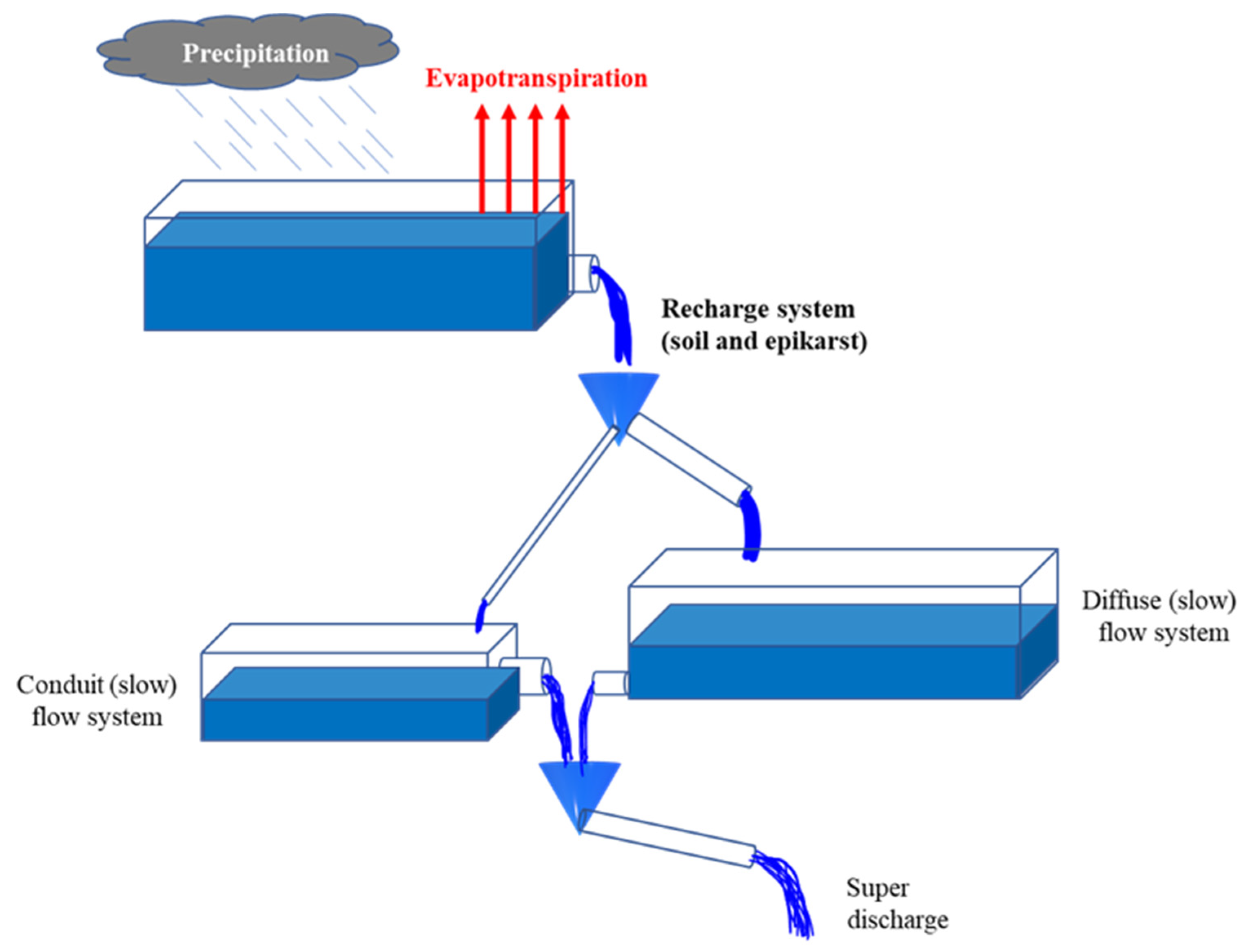
117]. Among the process-based methods, the lumped parameter model, RCD (recharge, conduit flow, diffuse flow), presented a suitable mathematical explanation of discharge and substance concentration. Refs. [9,21] elaborated on the fact that that karst vulnerability is not only a factor of recharge and discharge areas, but it also involves the individual springs in the discharge areas. As a global model, RCD cannot express the local factors related to groundwater recharge and point source pollution. This limitation can be avoided by integrating the catchment area’s vulnerability mapping (such as EPIK). In this literature review, among the karst vulnerability assessment, the RCD method presented an efficient explanation of the dynamic vulnerability distribution and temporal dependence of karst groundwater vulnerability.

5. Limitations and Future Directions

Significant developments have occurred in groundwater contamination vulnerability assessment in the last decade. Many integrated methods; GIS-based decision systems; and advanced techniques with combinations of index-based, statistical and/or process-based approaches have been employed to describe groundwater vulnerability. Despite these developments, some limitations still exist. The foundation of dynamic groundwater vulnerability relies on the recharge processes in unsaturated zones, which are the main pathways to carry the contaminants introduced on the land surface to the aquifers. In the last few decades, the main complexities arising in terms of assessing groundwater contamination vulnerability are climate change-induced uncertainties in general and human-induced impacts such as uncontrolled population growth in urban land use and pesticide load in agricultural fields in rural land use. To evaluate this complexity or identify the trend, almost all of the previous studies have been dependent upon deterministic methods, and they failed to consider stochasticity in the natural systems and the land use. Therefore, future studies should develop statistical methods based on stochastic approaches and process-based numerical techniques to trace the physical processes. Finally, a knowledge-based overlay and index-based method can be created for the zonation mapping of groundwater vulnerability. However, these data-driven processes have many limitations, such as the need for large datasets on controlling variables and contamination concentration, time consumption, complexity in geospatial evaluation, tracking the temporal aspects of the release of contaminants on the surface, and transportation through sub-surface flow. Therefore, identifying and setting up the time-dependent parameters, tracking the indicators, and looking at the proxies and their relationship with the groundwater contaminant concentration should be helpful tools to evaluate spatiotemporal groundwater vulnerability to contamination. For future studies, the following parameters and steps will be useful to develop a sophisticated model for groundwater vulnerability assessment.
Tracking the concentration of contaminants over a period depicts the temporal dependency (i.e., change detection over a month/season/year/longer period). These time-dependent changes are mainly based on anthropogenic activities on the Earth’s surface. Therefore, a more advanced assessment of land use and its variation over time is crucial to evaluating its sensitivity. Assessing the population growth and density over time will be a proxy for understanding the pollution load. More involvement of high-resolution time series and/or radar satellite images will be helpful. Tracking soil moisture could be a proxy for understanding the preferential flow. This is the primary transporter of agrochemicals under agricultural land use. Synthetic aperture radar (SAR) images will be a good option for tracking soil moisture over time and space. Slope is also one of the main associates in groundwater qualitative vulnerability assessment, but is widely neglected. Slope directly controls the rate of the soil’s percolation; surface runoff; and, indirectly, the soil moisture and groundwater recharge. Object-based image analysis (OBIA) can be used for land use classification instead of conventional pixel-based methods (i.e., supervised and unsupervised classification). OBIA is based on image segmentation, creating vector objects by clustering a small group of pixels. This technique is very useful for classifying agricultural fields and human settlements.

6. Conclusions

This paper presents a systematic review of the recent developments in the assessment of dynamic GW vulnerability to contamination. This review paper emphasized the time series analysis in the field of GW contamination vulnerability assessment conducted in the last decade. It was observed that quantitative approaches (i.e., statistical and process-based) have been the most popular for the assessment of GW qualitative vulnerability, followed by index-based approaches. The assessment approaches for GW contamination reviewed in this paper can be categorized into two groups: for resource protection and for source identification. Nitrate was the main indicator taken into consideration for the GW vulnerability assessment, and very few studies have concentrated on other contaminants like vanadium, ammonia, selenium, nitrogen, fluoride, chlorate, arsenic, some pesticides, etc. The countries studied in the research articles or case studies reviewed in this paper were primarily China and India, followed by some European countries and the rest of the world. This systematic review revealed that, among qualitative or overlay- and index-based methods such as DRASTIC and GOD, which were introduced during the late 1980s, are still popular choices for researchers. These methods have been modified or used alongside others to calculate the spatiotemporal risk of GW contamination. Over time, land use becomes an integral part of these methods to demonstrate the human involvement in the GW contamination. Due to advanced capabilities, GIS technology has become a crucial part of these GW vulnerability assessments. GIS is a unique tool which can be used to record, store, manipulate, and analyze the datasets and combine various data layers to demonstrate the vulnerability and demarcate the zones as per the GW quality. Sometimes, these methods are compared and validated with statistical tools such as kriging, PCA, and AHP. During the last decade, 1D, 2D, and 3D numerical models based on advection–dispersion equations have been used to identify the transport through the unsaturated as well as the saturated zones. Transport models such as HYDRUS-1D, MODFLOW, MODPATH, and MT3DMS have been found to be the most common and widely used methods.
All of the methods reviewed in this paper have their own advantages and limitations, as presented in Table 5, Table 6 and Table 7. Many fancy groundwater contamination assessment techniques which can demonstrate the dynamic vulnerability of the groundwater have been developed in the last decade. It can be concluded that many of the modeling techniques are lacking in terms of incorporating the foundation of the dynamic GW vulnerability, which relies on the recharge processes in unsaturated zones. There is a huge scope to improve the parameterization of the models in order to enable them to simulate the fate and transport of contaminants in saturated zones in a broader way. While dealing with the recharge, the surface water and groundwater interactions and their temporal variations should also be considered. It is also important to check the linearity or non-linearity of the dependent and predictor variables during the model execution procedure. In the assessment of intrinsic GW vulnerability, uncertainty is the main hindrance, and can never be eliminated. But this situation of uncertainty can be reduced, and assessment approaches can be improved by incorporating enhanced updated datasets, improved monitoring, and modern techniques. Holistic approaches need to be formulated to evaluate the groundwater contamination in an environment of changing climatic scenarios and uncertainties. Considering these fundamental situations, assessment techniques should present clear guidelines for sustainable groundwater management strategies.

Supplementary Materials

The following supporting information can be downloaded at: https://www.mdpi.com/article/10.3390/hydrology10090182/s1, Figure S1.: Statistical/Soft computing/Machine learning methods for GW contamination; Figure S2: Widely used Process-Based modelling techniques for GW contamination assessment; Table S1: Widely used Overlay and Index-based modelling techniques; Table S2: Search criteria and Boolean operators applied to Web of Science and ScienceDirect databases. (Porous media aquifers); Table S3: Search criteria and Boolean operators applied to Web of Science and ScienceDirect databases. (Karst aquifers); Table S4: Exclusion criteria followed by PRISMA for the need of this review.

Author Contributions

A.B.: conceptualization, methodology, original draft preparation; L.C.: supervision, reviewing and editing; N.J.: supervision and reviewing; L.G.: supervision, reviewing and editing; S.G.: supervision, conceptualization, methodology, reviewing and editing. All authors have read and agreed to the published version of the manuscript.

Funding

This research received no external funding.

Acknowledgments

The authors would like to acknowledge the support of Atlantic Technological University Sligo, Ireland, and funding from the CUA Bursary Scheme.

Conflicts of Interest

The authors declare no conflict of interest.

References

  1. Lall, U.; Josset, L.; Russo, T. A snapshot of the world’s groundwater challenges. Annu. Rev. Environ. Resour. 2020, 45, 171–194. [Google Scholar] [CrossRef]
  2. IGRAC. Groundwater Overview, Making the Invisible Visible. 2018. Available online: https://www.un-igrac.org/sites/default/files/resources/files/Groundwater%20overview%20-%20Making%20the%20invisible%20visible_Print.pdf (accessed on 29 July 2023).
  3. Dhenadhayalan, N.; Lin, K.C.; Saleh, T.A. Recent Advances in Functionalized Carbon Dots toward the Design of Efficient Materials for Sensing and Catalysis Applications. Small 2020, 16, e1905767. [Google Scholar] [CrossRef] [PubMed]
  4. Machiwal, D.; Jha, M.K.; Singh, V.P.; Mohan, C. Assessment and mapping of groundwater vulnerability to pollution: Current status and challenges. Earth Sci. Rev. 2018, 185, 901–927. [Google Scholar] [CrossRef]
  5. Machiwal, D.; Cloutier, V.; Güler, C.; Kazakis, N. A review of GIS-integrated statistical techniques for groundwater quality evaluation and protection. Environ. Earth Sci. 2018, 77, 681. [Google Scholar] [CrossRef]
  6. Ravbar, N.; Goldscheider, N. Proposed methodology of vulnerability and contamination risk mapping for the protection of karst aquifers in Slovenia (Predlog metodologije kartiranja ranljivosti in tveganja za onesnaženje voda za varovanje kraških vodonosnikov v Sloveniji). Acta Carsologica 2007, 36, 397–411. [Google Scholar]
  7. Stevenazzi, S.; Masetti, M.; Nghiem, S.V.; Sorichetta, A. Cartes de vulnérabilité des eaux souterraines déduites d’une method dépendante du temps utilisant des données satellitaires de scatteromètre. Hydrogeol. J. 2015, 23, 631–647. [Google Scholar] [CrossRef]
  8. Butscher, C.; Huggenberger, P. Intrinsic vulnerability assessment in karst areas: A numerical modeling approach. Water Resour. Res. 2008, 44. [Google Scholar] [CrossRef]
  9. Butscher, C.; Huggenberger, P. Enhanced vulnerability assessment in karst areas by combining mapping with modeling approaches. Sci. Total Environ. 2009, 407, 1153–1163. [Google Scholar] [CrossRef] [PubMed]
  10. Margat, J.; van der Gun, J. Groundwater around the World: A Geographic Synopsis; CRC Press: Boca Raton, FL, USA, 2013. [Google Scholar]
  11. Fetter, C.W. Applied Hydrogeology, 4th ed.; Prentice Hall: Hoboken, NJ, USA, 2001. [Google Scholar]
  12. Ghosh, N.C. Geogenic Contamination and Technologies for Safe Drinking Water Supply BT—Water and Sanitation in the New Millennium; Nath, K.J., Sharma, V.P., Eds.; Springer: New Delhi, India, 2017; pp. 81–95. [Google Scholar] [CrossRef]
  13. Bloomfield, J.P.; Williams, R.J.; Gooddy, D.C.; Cape, J.N.; Guha, P. Impacts of climate change on the fate and behaviour of pesticides in surface and groundwater—A UK perspective. Sci. Total Environ. 2006, 369, 163–177. [Google Scholar] [CrossRef]
  14. Kovalevskii, V.S. Effect of climate changes on groundwater. Water Resour. 2007, 34, 140–152. [Google Scholar] [CrossRef]
  15. Aureli, A.; Taniguchi, M. Groundwater Resources Assesment under the Pressures of Humanity and Climate Changes. Paris. 2006. Available online: https://iwlearn.net/resolveuid/01d776e51f524e6fa99c85b17686aece (accessed on 29 July 2023).
  16. Green, T.R. Linking Climate Change and Groundwater. In Integrated Groundwater Management: Concepts, Approaches and Challenges; Jakeman, A.J., Barreteau, O., Hunt, R.J., Rinaudo, J.D., Ross, A., Eds.; Springer: Berlin/Heidelberg, Germany, 2016; pp. 97–141. [Google Scholar] [CrossRef]
  17. Stigter, T.Y.; Ribeiro, L.; Dill, A.M.M.C. Evaluation of an intrinsic and a specific vulnerability assessment method in comparison with groundwater salinisation and nitrate contamination levels in two agricultural regions in the south of Portugal. Hydrogeol. J. 2006, 14, 79–99. [Google Scholar] [CrossRef]
  18. Margat, J. Vulnerabilite des Nappes d’eau Souterraine a la Pollution (Groundwater Vulnerability to Contamination); Bureau de Recherches Géologiques et Minières (BRGM): Orleans, France, 1968. [Google Scholar]
  19. Vrba, J.; Zaporozec, A. Guidebook on Mapping Groundwater Vulnerability; H. Heise: Hannover, Germany, 1994. [Google Scholar]
  20. National Research Council. Ground Water Vulnerability Assessment: Predicting Relative Contamination Potential Under Conditions of Uncertainty; The National Academies Press: Washington, DC, USA, 1993. [Google Scholar] [CrossRef]
  21. Butscher, C.; Huggenberger, P. Modeling the temporal variability of karst groundwater vulnerability, with implications for climate change. Environ. Sci. Technol. 2009, 43, 1665–1669. [Google Scholar] [CrossRef]
  22. Doerfliger, N.; Jeannin, P.-Y.; Zwahlen, F. Water Vulnerability Assessment in Karst Environments: A New Method of Defining Protection Areas Using a Multi-Attribute Approach and GIS Tools (EPIK Method); Springer: Berlin/Heidelberg, Germany, 1999. [Google Scholar]
  23. Gogu, R.C.; Dassargues, A. Current Trends and Future Challenges in Groundwater Vulnerability Assessment Using Overlay and Index Methods; Springer: Berlin/Heidelberg, Germany, 2000. [Google Scholar]
  24. Anderson, M.P.; Woessner, W.W. (Eds.) Chapter 1—Introduction. In Applied Groundwater Modeling; Academic Press: San Diego, CA, USA, 2002; pp. 1–11. [Google Scholar] [CrossRef]
  25. Boufekane, A.; Saighi, O. Application of Groundwater Vulnerability Overlay and Index Methods to the Jijel Plain Area (Algeria). Groundwater 2018, 56, 143–156. [Google Scholar] [CrossRef]
  26. Masetti, M.; Sterlacchini, S.; Ballabio, C.; Sorichetta, A.; Poli, S. Influence of threshold value in the use of statistical methods for groundwater vulnerability assessment. Sci. Total Environ. 2009, 407, 3836–3846. [Google Scholar] [CrossRef] [PubMed]
  27. Haan, C.T. Statistical Methods in Hydrology; Iowa State University Press: Ames, IA, USA, 1977. [Google Scholar]
  28. Sotornikova, R.; Vrba, J. The concept of vulnerability maps. In Proceedings of the International Conference on Vulnerability of Soil and Groundwater to Pollutants, The Hague, The Netherlands, 30 March–3 April 1987; pp. 471–476. [Google Scholar]
  29. Barbulescu, A. Assessing groundwater vulnerability: DRASTIC and DRASTIC-like methods: A review. Water 2020, 12, 1356. [Google Scholar] [CrossRef]
  30. Haghbin, M.; Sharafati, A.; Dixon, B.; Kumar, V. Application of Soft Computing Models for Simulating Nitrate Contamination in Groundwater: Comprehensive Review, Assessment and Future Opportunities. Arch. Comput. Methods Eng. 2020, 28, 3569–3591. [Google Scholar] [CrossRef]
  31. Liberati, A.; Altman, D.G.; Tetzlaff, J.; Mulrow, C.; Gøtzsche, P.C.; Ioannidis, J.P.A.; Clarke, M.; Devereaux, P.J.; Kleijnen, J.; Moher, D. The PRISMA statement for reporting systematic reviews and meta-analyses of studies that evaluate health care interventions: Explanation and elaboration. Ann. Intern. Med. 2009, 62, E1–E34. [Google Scholar] [CrossRef]
  32. Nan, Z.; Bo, L.; Changlai, X. Spatio-Temporal variation of groundwater contamination using IEA-UEF in urban areas of Jilin City, North-eastern China. Water Sci. Technol. Water Supply 2016, 16, 1277–1286. [Google Scholar] [CrossRef]
  33. Mahmood, K.; Ul-Haq, Z.; Batool, S.A.; Rana, A.D.; Tariq, S. Application of temporal GIS to track areas of significant concern regarding groundwater contamination. Environ. Earth Sci 2016, 75, 33. [Google Scholar] [CrossRef]
  34. Chaturvedi, A.; Bhattacharjee, S.; Singh, A.K.; Kumar, V. A new approach for indexing groundwater heavy metal pollution. Ecol. Indic. 2018, 87, 323–331. [Google Scholar] [CrossRef]
  35. Misi, A.; Gumindoga, W.; Hoko, Z. An assessment of groundwater potential and vulnerability in the Upper Manyame Sub-Catchment of Zimbabwe. Phys. Chem. Earth 2018, 105, 72–83. [Google Scholar] [CrossRef]
  36. Duttagupta, S.; Mukherjee, A.; Das, K.; Dutta, A.; Bhattacharya, A.; Bhattacharya, J. Groundwater vulnerability to pesticide pollution assessment in the alluvial aquifer of Western Bengal basin, India using overlay and index method. Geochemistry 2020, 80, 125601. [Google Scholar] [CrossRef]
  37. Vu, T.D.; Ni, C.F.; Li, W.C.; Truong, M.H. Modified index-overlay method to assess spatial-temporal variations of groundwater vulnerability and groundwater contamination risk in areas with variable activities of agriculture developments. Water 2019, 11, 2492. [Google Scholar] [CrossRef]
  38. Nistor, M.M. Vulnerability of groundwater resources under climate change in the Pannonian basin. Geo-Spat. Inf. Sci. 2019, 22, 345–358. [Google Scholar] [CrossRef]
  39. Haidu, I.; Nistor, M.M. Groundwater vulnerability assessment in the Grand Est region, France. Quat. Int. 2020, 547, 86–100. [Google Scholar] [CrossRef]
  40. Bahrami, M.; Zarei, A.R.; Rostami, F. Temporal and spatial assessment of groundwater contamination with nitrate by nitrate pollution index (NPI) and GIS (case study: Fasarud Plain, southern Iran). Env. Geochem Health 2020, 42, 3119–3130. [Google Scholar] [CrossRef] [PubMed]
  41. Mendes, M.P.; Ribeiro, L. Nitrate probability mapping in the northern aquifer alluvial system of the river Tagus (Portugal) using Disjunctive Kriging. Sci. Total Environ. 2010, 408, 1021–1034. [Google Scholar] [CrossRef]
  42. Kurunc, A.; Ersahin, S.; Sonmez, N.K.; Kaman, H.; Uz, I.; Uz, B.Y.; Aslan, G.E. Seasonal changes of spatial variation of some groundwater quality variables in a large irrigated coastal Mediterranean region of Turkey. Sci. Total Environ. 2016, 554–555, 53–63. [Google Scholar] [CrossRef] [PubMed]
  43. Di Guardo, A.; Finizio, A. A moni-modelling approach to manage groundwater risk to pesticide leaching at regional scale. Sci. Total Environ. 2016, 545–546, 200–209. [Google Scholar] [CrossRef]
  44. Di Guardo, A.; Finizio, A. A client-server software for the identification of groundwater vulnerability to pesticides at regional level. Sci. Total Environ. 2015, 530–531, 247–256. [Google Scholar] [CrossRef]
  45. Chitsazan, M.; Tabari, M.M.R.; Eilbeigi, M. Analysis of temporal and spatial variations in groundwater nitrate and development of its pollution plume: A case study in Karaj aquifer. Environ. Earth Sci. 2017, 76, 391. [Google Scholar] [CrossRef]
  46. Naaz, A.; Kumar, B.; Narayan, C.; Shukla, K.; Anshumali. Assessment of fluoride pollution in groundwaters of arid and semi-arid regions of tonalite–trondjhemite series in central India. Expo Health 2015, 7, 545–556. [Google Scholar] [CrossRef]
  47. He, X.; Qian, J.; Liu, Z.; Lu, Y.; Ma, L.; Zhao, W.; Kang, B. Temporal-Spatial Evolution of Groundwater Nitrogen Pollution Over Seven Years in a Highly Urbanized City in the Southern China. Bull. Environ. Contam. Toxicol. 2017, 99, 753–759. [Google Scholar] [CrossRef] [PubMed]
  48. Richards, G.; Gilmore, T.E.; Mittelstet, A.R.; Messer, T.L.; Snow, D.D. Baseflow nitrate dynamics within nested watersheds of an agricultural stream in Nebraska, USA. Agric. Ecosyst. Environ. 2021, 308, 107223. [Google Scholar] [CrossRef]
  49. Arslan, H.; Turan, N.A.; Demir, Y.; Güngör, A.; Cemek, B. Assessment of spatial and seasonal changes in groundwater nitrate pollution of agricultural lands through ordinary and indicator kriging techniques. Arch. Agron. Soil Sci. 2017, 63, 907–917. [Google Scholar] [CrossRef]
  50. Ghosh, M.; Pal, D.K.; Santra, S.C. Spatial mapping and modeling of arsenic contamination of groundwater and risk assessment through geospatial interpolation technique. Environ. Dev. Sustain. 2020, 22, 2861–2880. [Google Scholar] [CrossRef]
  51. Menchen, A.; las Heras, J.D.; Alday, J.J.G. Pesticide contamination in groundwater bodies in the Júcar River European Union Pilot Basin (SE Spain). Environ. Monit Assess 2017, 189, 146. [Google Scholar] [CrossRef]
  52. Chen, S.; Wu, W.; Hu, K.; Li, W. The effects of land use change and irrigation water resource on nitrate contamination in shallow groundwater at county scale. Ecol. Complex. 2010, 7, 131–138. [Google Scholar] [CrossRef]
  53. Boy-Roura, M.; Menció, A.; Mas-Pla, J. Temporal analysis of spring water data to assess nitrate inputs to groundwater in an agricultural area (Osona, NE Spain). Sci. Total Environ. 2013, 452–453, 433–445. [Google Scholar] [CrossRef]
  54. Li, Q.; Zhang, H.; Guo, S.; Fu, K.; Liao, L.; Xu, Y.; Cheng, S. Groundwater pollution source apportionment using principal component analysis in a multiple land-use area in southwestern China. Environ. Sci. Pollut. Res. 2020, 27, 9000–9011. [Google Scholar] [CrossRef]
  55. Azzellino, A.; Colombo, L.; Lombi, S.; Marchesi, V.; Piana, A.; Andrea, M.; Alberti, L. Groundwater diffuse pollution in functional urban areas: The need to define anthropogenic diffuse pollution background levels. Sci. Total Environ. 2019, 656, 1207–1222. [Google Scholar] [CrossRef]
  56. Mastrocicco, M.; Di Giuseppe, D.; Vincenzi, F.; Colombani, N.; Castaldelli, G. Chlorate origin and fate in shallow groundwater below agricultural landscapes. Environ. Pollut. 2017, 231, 1453–1462. [Google Scholar] [CrossRef]
  57. Jung, H.W.; Yun, S.T.; Kim, K.H.; Oh, S.S.; Kang, K.G. Role of an impermeable layer in controlling groundwater chemistry in a basaltic aquifer beneath an agricultural field, Jeju Island, South Korea. Appl. Geochem. 2014, 45, 82–93. [Google Scholar] [CrossRef]
  58. Machiwal, D.; Jha, M.K. Identifying sources of groundwater contamination in a hard-rock aquifer system using multivariate statistical analyses and GIS-based geostatistical modeling techniques. J. Hydrol. Reg. Stud. 2015, 4, 80–110. [Google Scholar] [CrossRef]
  59. Chatterjee, A.; Sarah, S.; Sreedevi, P.D.; Selles, A.; Ahmed, S. Demarcation of fluoride vulnerability zones in granitic aquifer, semi-arid region, Telengana, India. Arab. J. Geosci. 2017, 10, 558. [Google Scholar] [CrossRef]
  60. Jampani, M.; Huelsmann, S.; Liedl, R.; Sonkamble, S.; Ahmed, S.; Amerasinghe, P. Spatio-temporal distribution and chemical characterization of groundwater quality of a wastewater irrigated system: A case study. Sci. Total Environ. 2018, 636, 1089–1098. [Google Scholar] [CrossRef]
  61. Bro, R. Chemometrics and Intelligent Laboratory Systems Tutorial PARAFAC. Tutorial and Applications; Elsevier BV: Amsterdam, The Netherlands, 1997. [Google Scholar]
  62. Mellor, F.P.; Cey, E.E. Using generalized additive mixed models to assess spatial, temporal, and hydrologic controls on bacteria and nitrate in a vulnerable agricultural aquifer. J. Contam. Hydrol. 2015, 182, 104–116. [Google Scholar] [CrossRef] [PubMed]
  63. Wood, S.N. Generalized Additive Models: An Introduction with R; CRC Press: Boca Raton, FL, USA, 2017. [Google Scholar]
  64. Wang, S.; Tang, C.; Song, X.; Yuan, R.; Han, Z.; Pan, Y. Factors contributing to nitrate contamination in a groundwater recharge area of the North China Plain. Hydrol. Process. 2016, 30, 2271–2285. [Google Scholar] [CrossRef]
  65. Cao, Y.; Tang, C.; Song, X.; Liu, C.; Zhang, Y. Residence time as a key for comprehensive assessment of the relationship between changing land use and nitrates in regional groundwater systems. Environ. Sci. Process. Impacts 2013, 15, 876–885. [Google Scholar] [CrossRef]
  66. Wang, S.; Tang, C.; Song, X.; Wang, Q.; Zhang, Y.; Yuan, R. The impacts of a linear wastewater reservoir on groundwater recharge and geochemical evolution in a semi-arid area of the Lake Baiyangdian watershed, North China Plain. Sci. Total Environ. 2014, 482–483, 325–335. [Google Scholar] [CrossRef]
  67. Zhang, W.; Cheng, J.H.; Xian, Q.S.; Cui, J.F.; Tang, X.Y.; Wang, G.X. Dynamics and sources of colloids in shallow groundwater in lowland wells and fracture flow in sloping farmland. Water Res. 2019, 156, 252–263. [Google Scholar] [CrossRef]
  68. McLean, M.I.; Evers, L.; Bowman, A.W.; Bonte, M.; Jones, W.R. Statistical modelling of groundwater contamination monitoring data: A comparison of spatial and spatiotemporal methods. Sci. Total Environ. 2019, 652, 1339–1346. [Google Scholar] [CrossRef] [PubMed]
  69. Srivastava, D.; Singh, R.M. Breakthrough Curves Characterization and Identification of an Unknown Pollution Source in Groundwater System Using an Artificial Neural Network (ANN). Environ. Forensics 2014, 15, 175–189. [Google Scholar] [CrossRef]
  70. Pan, Z.; Lu, W.; Chang, Z.; Wang, H. Simultaneous identification of groundwater pollution source spatial–temporal characteristics and hydraulic parameters based on deep regularization neural network-hybrid heuristic algorithm. J. Hydrol. 2021, 600, 126586. [Google Scholar] [CrossRef]
  71. Huan, H.; Li, X.; Zhou, J.; Liu, W.; Li, J.; Liu, B.; Xi, B.; Jiang, Y. Groundwater pollution early warning based on QTR model for regional risk management: A case study in Luoyang city, China. Environ. Pollut. 2020, 259, 113900. [Google Scholar] [CrossRef] [PubMed]
  72. Chaudhuri, S.; Ale, S. Evaluation of Long-Term (1960–2010) Groundwater Fluoride Contamination in Texas. J. Environ. Qual. 2014, 43, 1404–1416. [Google Scholar] [CrossRef]
  73. Moran, P.A.P. Notes on Continuous Stochastic Phenomena. Biometrika 1950, 37, 17–23. [Google Scholar] [CrossRef]
  74. Chaudhuri, S.; Ale, S.; DeLaune, P.; Rajan, N. Spatio-temporal Variability of Groundwater Nitrate Concentration in Texas: 1960 to 2010. J. Environ. Qual 2012, 41, 1806–1817. [Google Scholar] [CrossRef] [PubMed]
  75. Bashi-Azghadi, S.N.; Kerachian, R.; Bazargan-Lari, M.R.; Nikoo, M.R. Pollution source identification in groundwater systems: Application of regret theory and Bayesian networks. Iran. J. Sci. Technol.—Trans. Civ. Eng. 2016, 40, 241–249. [Google Scholar] [CrossRef]
  76. Stumpp, C.; Żurek, A.J.; Wachniew, P.; Gargini, A.; Gemitzi, A.; Filippini, M.; Witczak, S. A decision tree tool supporting the assessment of groundwater vulnerability. Environ. Earth Sci. 2016, 75, 1057. [Google Scholar] [CrossRef]
  77. Ferreira, D.; Almeida, J.; Simes, M.; PrezMartin, M. Agricultural practices and geostatistical evaluation of nitrate pollution of groundwater in the Júcar River Basin District, Spain. Emir. J. Food Agric. 2016, 28, 415. [Google Scholar] [CrossRef]
  78. Pérez-Martín, M.A. Distributed Simulation Model of the Hydrological Cycle and Water Quality, Integrated in Geographic Information Systems for Large Basins. Contribution to the Analysis of Pressures and Impacts of the Water Framework Directive; Modelo Distribuido de Simulac; Universidad Politécnica de Valência: Valencia, Spain, 2005. [Google Scholar]
  79. Kim, H.; Sandersen, P.B.; Jakobsen, R.; Kallesøe, A.J.; Claes, N.; Blicher-Mathiesen, G.; Foged, N.; Aamand, J.; Hansen, B. A 3D hydrogeochemistry model of nitrate transport and fate in a glacial sediment catchment: A first step toward a numerical model. Sci. Total Environ. 2021, 776, 146041. [Google Scholar] [CrossRef]
  80. Mich el McDonald, G.; Harbaugh, A.W. Techniques of Water-Resources Investigations of the Uni tes Geological Survey, a Modu Finite-Diffe; USGS Publications: Denver, CO, USA, 1988.
  81. Wellman, T.P.; Kauffman, L.; Clark, B. A zonal evaluation of intrinsic susceptibility in selected principal aquifers of the United States. J. Hydrol. 2012, 440–441, 36–51. [Google Scholar] [CrossRef]
  82. Zhang, H.; Yang, R.; Wang, Y.; Ye, R. The evaluation and prediction of agriculture-related nitrate contamination in groundwater in Chengdu Plain, southwestern China. Hydrogeol. J. 2019, 27, 785–799. [Google Scholar] [CrossRef]
  83. Yang, L.; Zheng, C.; Andrews, C.B.; Wang, C. Applying a Regional Transport Modeling Framework to Manage Nitrate Contamination of Groundwater. Groundwater 2021, 59, 292–307. [Google Scholar] [CrossRef]
  84. Shaffer, M.J.; Halvorson, A.D. Nitrate Leaching and Economic Analysis Package (NLEAP): Chapter 13 Model Description and Application; Soil Science Society of America: Madison, WI, USA, 1991. [Google Scholar]
  85. Li, Z.; Wen, X.; Hu, C.; Li, X.; Li, S.; Zhang, X.; Hu, B. Regional simulation of nitrate leaching potential from winter wheat-summer maize rotation croplands on the North China Plain using the NLEAP-GIS model. Agric. Ecosyst. Environ. 2020, 294, 106861. [Google Scholar] [CrossRef]
  86. Kourakos, G.; Klein, F.; Cortis, A.; Harter, T. A groundwater nonpoint source pollution modeling framework to evaluate long-term dynamics of pollutant exceedance probabilities in wells and other discharge locations. Water Resour. Res. 2012, 48. [Google Scholar] [CrossRef]
  87. Bancheri, M.; Coppola, A.; Basile, A. A new transfer function model for the estimation of non-point-source solute travel times. J. Hydrol. 2021, 598, 126157. [Google Scholar] [CrossRef]
  88. Akhavan, S.; Abedi-Koupai, J.; Mousavi, S.F.; Afyuni, M.; Eslamian, S.S.; Abbaspour, K.C. Application of SWAT model to investigate nitrate leaching in Hamadan-Bahar Watershed, Iran. Agric. Ecosyst. Environ. 2010, 139, 675–688. [Google Scholar] [CrossRef]
  89. Kao, Y.H.; Liu, C.W.; Jang, C.S.; Zanh, S.W.; Lin, K.H. Assessment of nitrogen contamination of groundwater in paddy and upland fields. Paddy Water Environ. 2011, 9, 301–307. [Google Scholar] [CrossRef]
  90. Parkhurst, L.; Appelo, C.A.J. User’s Guide to Phreeqc (Version 2) a Computer Program for Speciation, Batch-Reaction, One-Dimensional Transport, And Inverse Geochemical Calculations. Water Resour. Investig. Rep. 1999, 99, 312. [Google Scholar]
  91. Lin, J.H.-C.; Richards, D.R.; Yeh, W.G.-T.; Cheng, J.-R.; Cheng, H.-P.; Jones, N.L. FEMWATER: A Three-Dimensional Finite Element Computer Model for Simulating Density-Dependent Flow and Transport in Variably Saturated Media; U.S. Army Engineer Waterways Experiment Station: Vicksburg, MS, USA, 1997.
  92. Llopis-Albert, C.; Palacios-Marqués, D.; Merigó, J.M. A coupled stochastic inverse-management framework for dealing with nonpoint agriculture pollution under groundwater parameter uncertainty. J. Hydrol. 2014, 511, 10–16. [Google Scholar] [CrossRef]
  93. Peña-Haro, S.; Pulido-Velazquez, M.; Sahuquillo, A. A hydro-economic modelling framework for optimal management of groundwater nitrate pollution from agriculture. J. Hydrol. 2009, 373, 193–203. [Google Scholar] [CrossRef]
  94. Zhang, Z.; Chen, X.; Cheng, Q.; Li, S.; Yue, F.; Peng, T.; Waldron, S.; Oliver, D.M.; Soulsby, C. Coupled hydrological and biogeochemical modelling of nitrogen transport in the karst critical zone. Sci. Total Environ. 2020, 732, 138902. [Google Scholar] [CrossRef]
  95. Bailey, R.T.; Gates, T.K.; Ahmadi, M. Simulating reactive transport of selenium coupled with nitrogen in a regional-scale irrigated groundwater system. J. Hydrol. 2014, 515, 29–46. [Google Scholar] [CrossRef]
  96. Datta, B.; Chakrabarty, D.; Dhar, A. Identification of unknown groundwater pollution sources using classical optimization with linked simulation. J. Hydro-Environ. Res. 2011, 5, 25–36. [Google Scholar] [CrossRef]
  97. Voss, C.I.; Florida, T.A.F.B. A Finite-Element Simulation Model for Saturated-Unsaturated, Fluid-Density-Dependent Groundwater Flow with Energy Transport or Chemically-Reactive Single-Species Solute Transport. Water Resour. Investig. Rep. 1984, 84, 4369. [Google Scholar]
  98. Vesselinov, V.V.; Alexandrov, B.S.; O’Malley, D. Contaminant source identification using semi-supervised machine learning. J. Contam Hydrol. 2018, 212, 134–142. [Google Scholar] [CrossRef]
  99. Belouchrani, A.; Abed-Meraim, K.; Cardoso, J.-F.; Moulines, E. A blind source separation technique using second-order statistics. IEEE Trans. Signal Process. 1997, 45, 434–444. [Google Scholar] [CrossRef]
  100. Lee, D.; Seung, H.S. Learning the parts of objects by non-negative matrix factorization. Lett. Nat. 1999, 401, 788–791. [Google Scholar] [CrossRef]
  101. Alexandrov, S.; Vesselinov, V.V. Blind source separation for groundwater pressure analysis based on nonnegative matrix factorization. Water Resour. Res. 2014, 50, 7332–7347. [Google Scholar] [CrossRef]
  102. Bottrell, S.H.; Ford, D.; Williams, P. Karst Geomorphology and Hydrology; John Wiley & Sons: Hoboken, NJ, USA, 1991; Volume 157. [Google Scholar] [CrossRef]
  103. Albuquerque, M.T.D.; Sanz, G.; Oliveira, S.F.; Martínez-Alegría, R.; Antunes, I.M.H.R. Spatio-Temporal Groundwater Vulnerability Assessment—A Coupled Remote Sensing and GIS Approach for Historical Land Cover Reconstruction. Water Resour. Manag. 2013, 27, 4509–4526. [Google Scholar] [CrossRef]
  104. Elias, D.; Angeliki, M.; Vasiliki, M.; Maria, T.; Christina, Z. Geospatial Investigation into Groundwater Pollution and Water Quality Supported by Satellite Data: A Case Study from the Evros River (Eastern Mediterranean). Pure Appl. Geophys. 2012, 171, 977–995. [Google Scholar] [CrossRef]
  105. Vías, M.; Andreo, B.; Perles, M.J.; Carrasco, F.; Vadillo, I.; Jiménez, P. Proposed method for groundwater vulnerability mapping in carbonate (karstic) aquifers: The COP method. Hydrogeol. J. 2006, 14, 912–925. [Google Scholar] [CrossRef]
  106. Turpaud, P.; Zini, L.; Ravbar, N.; Cucchi, F.; Petrič, M.; Urbanc, J. Development of a Protocol for the Karst Water Source Protection Zoning: Application to the Classical Karst Region (NE Italy and SW Slovenia). Water Resour. Manag. 2018, 32, 1953–1968. [Google Scholar] [CrossRef]
  107. Živanović, V.; Jemcov, I.; Dragišić, V.; Atanacković, N.; Magazinović, S. Karst groundwater source protection based on the time-dependent vulnerability assessment model: Crnica springs case study, Eastern Serbia. Environ. Earth Sci. 2016, 75, 1224. [Google Scholar] [CrossRef]
  108. Živanović, V.; Atanacković, N.; Stojadinović, S. Vulnerability Assessment as a Basis for Sanitary Zone Delineation of Karst Groundwater Sources—Blederija Spring Case Study. Water 2021, 13, 2775. [Google Scholar] [CrossRef]
  109. Dedewanou, M.; Binet, S.; Rouet, J.L.; Coquet, Y.; Bruand, A.; Noel, H. Groundwater Vulnerability and Risk Mapping Based on Residence Time Distributions: Spatial Analysis for the Estimation of Lumped Parameters. Water Resour. Manag. 2015, 29, 5489–5504. [Google Scholar] [CrossRef]
  110. Hakoun, V.; Orban, P.; Dassargues, A.; Brouyère, S. Factors controlling spatial and temporal patterns of multiple pesticide compounds in groundwater (Hesbaye chalk aquifer, Belgium). Environ. Pollut. 2017, 223, 185–199. [Google Scholar] [CrossRef]
  111. Romshoo, S.A.; Dar, R.A.; Murtaza, K.O.; Rashid, I.; Dar, F.A. Hydrochemical characterization and pollution assessment of groundwater in Jammu Siwaliks, India. Environ. Monit. Assess. 2017, 189, 122. [Google Scholar] [CrossRef]
  112. Torres, N.I.; Yu, X.; Padilla, I.Y.; Macchiavelli, R.E.; Ghasemizadeh, R.; Kaeli, D.; Cordero, J.F.; Meeker, J.D.; Alshawabkeh, A.N. The influence of hydrogeological and anthropogenic variables on phthalate contamination in eogenetic karst groundwater systems. Environ. Pollut. 2018, 237, 298–307. [Google Scholar] [CrossRef] [PubMed]
  113. Yu, X.; Ghasemizadeh, R.; Padilla, I.; Irizarry, C.; Kaeli, D.; Alshawabkeh, A. Spatiotemporal changes of CVOC concentrations in karst aquifers: Analysis of three decades of data from Puerto Rico. Sci. Total Environ. 2015, 511, 1–10. [Google Scholar] [CrossRef] [PubMed]
  114. Butscher, C.; Huggenberger, P. Implications for karst hydrology from 3D geological modeling using the aquifer base gradient approach. J. Hydrol. 2007, 342, 184–198. [Google Scholar] [CrossRef]
  115. Epting, J.; Page, R.M.; Auckenthaler, A.; Huggenberger, P. Process-based monitoring and modeling of Karst springs—Linking intrinsic to specific vulnerability. Sci. Total Environ. 2018, 625, 403–415. [Google Scholar] [CrossRef] [PubMed]
  116. Li, Q.; Qi, J.; Xing, Z.; Li, S.; Jiang, Y.; Danielescu, S.; Zhu, H.; Wei, X.; Meng, F.-R. An approach for assessing impact of land use and biophysical conditions across landscape on recharge rate and nitrogen loading of groundwater. Agric. Ecosyst. Environ. 2014, 196, 114–124. [Google Scholar] [CrossRef]
  117. Kavouri, P.; Karatzas, G.P.; Plagnes, V. Un modèle couple d’écoulement d’eau souterraine et d’une méthodologie de cartographie de la vulnérabilité pour la gestion des terrains karstiques. Hydrogeol. J. 2017, 25, 1301–1317. [Google Scholar] [CrossRef]
  118. Diersch, H.-J.G. Heat Transport in Porous Media. In FEFLOW; Springer: Berlin/Heidelberg, Germany, 2014; pp. 673–709. [Google Scholar] [CrossRef]
  119. Binet, S.; Joigneaux, E.; Pauwels, H.; Albéric, P.; Fléhoc, C.; Bruand, A. Water exchange, mixing and transient storage between a saturated karstic conduit and the surrounding aquifer: Groundwater flow modeling and inputs from stable water isotopes. J. Hydrol. 2017, 544, 278–289. [Google Scholar] [CrossRef]
  120. Surdyk, N.; Gutierrez, A.; Baran, N.; Thiéry, D. A lumped model to simulate nitrate concentration evolution in groundwater at catchment scale. J. Hydrol. 2021, 596, 125696. [Google Scholar] [CrossRef]
  121. Thiery, D.; Seguin, J.-J. Modélisation Globale Des Transferts De Nitrates Dans Un Bassin Hydrogéologique Pour Prévoir L’évolution Des Concentrations Dans Les Eaux Souterraines Description Du Modèle BICHE Trois Exemples D’application; Bureau De Recherches Géologiques Et Minières Service Géologique National Département Eau: Orleans, France, 1985.
Figure 1. Methodology of the systematic literature review using a PRISMA flow diagram.
Hydrology 10 00182 g001
Figure 2. Flowchart for the overlay and index models used to assess groundwater contamination.
Hydrology 10 00182 g002
Figure 3. General flowchart for the statistical model to assess groundwater contamination.
Hydrology 10 00182 g003
Figure 4. A general flow diagram depicting a simulation for a process-based model.
Hydrology 10 00182 g004
Figure 5. Framework for simulation initialization of NPSAT, modified after [86].
Hydrology 10 00182 g005
Figure 6. Framework for model initialization and the estimation of model parameter values, modified after [95].
Hydrology 10 00182 g006
Figure 7. Schematic representation of the model setup, modified after [21].
Hydrology 10 00182 g007
Figure 8. Flow diagram of the BICHE model, modified after [120].
Hydrology 10 00182 g008
Table 1. Summary of the index-based models.
Author(s)Aquifer TypeContaminantPurpose of the StudySources of PollutionLocation of InterestMethods Used
[32]AlluvialMiscellaneousResource protectionGeneralJilin City, ChinaIEA-UEF
[33]AlluvialMiscellaneousResource protectionGeneralLahore, PakistanWater quality index (WQI)
[34]AlluvialHeavy metalResource protectionUrban effluentsSubarnarekha River Basin, Indiam-HPI
[35]BasementAmmoniaResource protectionUrban effluentsUpper Manyame Catchment, ZimbabweGOD, PCA
[37]Sedimentary NitrateResource protectionAgriculturePingtung plain, TaiwanDRASTIC and AHP
[38]AlluvialGeneralResource protectionAgriculturePannonian basin ** GVI
[36]AlluvialPesticidesResource protectionAgricultureWestern Bengal Basin, IndiaDRASTIC
[39]MiscellaneousNitrateResource protectionMiscellaneousGrand Est region, FranceGVI
[40]AlluvialNitrateResource protectionAgricultureFasarud Plain, southern IranNitrate pollution index
** Slovakia, Ukraine, Hungary, Romania, Austria, Slovenia, Croatia, Bosnia and Herzegovina, Serbia, Montenegro.
Table 2. Summary of the statistical models of GW contamination.
Author(s)Aquifer TypeContaminantPurpose of the StudySources of PollutionLocation of InterestMethods Used
[41]Alluvial NitrateResource protectionAgriculturePortugalDK
[52]AlluvialNitrateResource protectionAgricultureChinaSemivariogram (Kriging)
[53]SedimentaryNitrateResource protectionAgricultureSpainSemivariogram (Kriging)
[57]VolcanicNitrate and VanadiumResource protectionAgricultureSouth KoreaCPCA and ROBPCA
[72]SedimentaryFluorideResource protectionAgricultureUSALISA
[69]GeneralGeneralSource IdentificationGeneralNot location specificANN
[62]AlluvialNitrateResource protectionAgricultureCanadaGAMMs/regression models
[58]BasementMiscellaneousSource identificationGeneralIndiaGQI, HCA, PCA
[46]AlluvialFluorideResource protectionBedrockIndiaPCA and Varimax Rotation
[7]AlluvialNitrateResource protectionBedrock and land useItalyWofE
[42]AlluvialNitrateResource protectionAgricultureTurkeyKriging
[43]AlluvialTba, Gly, Pend, s-Met, Cpyr and d-TbaSource IdentificationAgricultureItalymoni-modeling approach
[75]AlluvialGeneralSource IdentificationGeneralIranRegret Theory and Bayesian Networks
[76]GeneralGeneralResource protectionGeneralNot location specificDecision tree
[64]SedimentaryNitrateResource protectionAgricultureChinaMultiple regression model
[77]SedimentaryNitrateResource protectionAgricultureSpainSpatial variograms
[56]SedimentaryChlorateResource protectionAgricultureItalyPCA
[59]BasementFluorideSource IdentificationBedrockIndiaFA
[47]VolcanicNitrate, Nitrite, and AmmoniumResource protectionAgrochemicals and urban wastesChinaKriging
[49]AlluvialNitrateResource protectionAgricultureTurkeyOK and IK
[45]SedimentaryNitrateResource protectionUrban, agricultural and industrial wastewaterIranOK
[51]SedimentaryPesticidesResource protectionAgricultureSpainPCA
[60]BasementMiscellaneousResource protectionAgricultureIndiaFA, HCA and PARAFAC
[55]SedimentaryMiscellaneousResource protectionUrban and industrial wastewaterItalyPCA and FA
[68]GeneralGeneralSource IdentificationGeneralNot location specificSpatial Kriging
[67] SedimentaryColloidsSource IdentificationAgricultureChinaMulti-linear regression
[71] SedimentaryGeneralResource protectionGeneralChinaQTR model
[50] AlluvialArsenicSource IdentificationBedrockIndiaThiessen polygon and Kriging
[54]AlluvialNitrate, Nitrite, and AmmoniumSource IdentificationUrban, agricultural and industrial wastewaterChinaPCA
[48]AlluvialNitrateSource IdentificationAgricultureUSAKriging
[79]SedimentaryNitrateSource IdentificationAgricultureDenmarkK-means
[70]GeneralGeneralSource IdentificationGeneralNot location specificNeural network-hybrid heuristic algorithm
Table 3. Summary of the process-based models.
Author(s)Aquifer TypeContaminantPurpose of the StudySources of PollutionLocation of InterestMethods Used
[88]AlluvialNitrateResource protectionAgricultureHamadan–Bahar Watershed, IranSWAT
[96]GeneralGeneralSource identificationGeneralNot location-specificSUTRA, OSIM
[89]AlluvialNitrogenResource protectionAgricultureChoushui river alluvial fan, TaiwanPHREEQC, FEMWATER
[81]MiscellaneousGeneralResource protectionGeneralSelected principal aquifers of the United StatesMODFLOW, MODPATH
[86]AlluvialNitrateSource identificationAgricultureTule River groundwater sub-basin, CaliforniaNPSAT
[92]GeneralNitrateSource identificationAgricultureNot location-specificStochastic inverse model
[95]AlluvialSelenium, NitrogenResource protectionAgricultureArkansas River Valley in ColoradoUZF-RT3D
[98]GeneralGeneralSource identificationGeneralNot location-specificNMFk
[82]AlluvialNitrateResource protectionAgricultureChengdu Plain, southwestern ChinaMODFLOW and MT3DMS
[85]AlluvialNitrateSource identificationAgricultureJing-Jin-Ji region, ChinaNLEAP-GIS
[94]AlluvialNitrateResource protectionAgricultureDeyang city, China HYDRUS-1D and MT3DMS
[87]GeneralNitrates and PesticidesResource protectionAgricultureNot location-specificTFM-ext
[83]AlluvialNitrateResource protectionAgricultureDagu Aquifer, ChinaNLEAP, MODFLOW, MT3DMS
Table 4. Summary of the karst vulnerability assessment methods.
Author(s)ContaminantPurpose of the StudySources of PollutionLocation of InterestMethods Used
Overlay and index-based methods
[6]General Source protectionGeneralSloveniaSlovene Approach
[104]General Resource protectionAgrochemicals and urban wastesThe Evros river catchment (Bulgaria, Turkey, and Greece)Geographically weighted regression
[103]NitrateResource protectionAgricultureÁgueda River catchment (Spain and Portugal)DRASTIC and SI
[107]GeneralSource protectionGeneralSerbiaTDM
[106]GeneralResource protectionGeneralNE Italy and SW SloveniaSlovene Approach
[108]GeneralSource protectionGeneralSerbiaCOP + K and TDM
Statistical methods
[109]GeneralResource protectionGeneralNot location specificRTD
[113]CVOCsResource protectionGeneralIslandsIDW
[110]Bentazone, atrazine, diuron and simazine, DEA, and BAMResource protectionAgricultureBelgiumPCA
[111]SulfateSource identificationBedrockIndiaFA and HCA
[112]PhthalatesSource protectionIndustrialPuerto RicoIDW and logistic regression model
Process-based methods
[21]General Resource protectionGeneralSwitzerlandRCD-seasonal
[9]GeneralSource protectionGeneralSwitzerlandABG, EPIK, and RCD
[116]NitrogenResource protectionAgricultureCanadaSWAT
[119]GeneralResource protectionGeneralFranceFeflow
[117]GeneralResource protectionGeneralGreeceFeflow, PaPRIKa
[115]GeneralSource protectionGeneralSwitzerland3D geological model and RCD
[120]NitrateResource protectionAgricultureFranceBICHE
Table 5. Key features and limitations of the index-based models.
ModelsKey FeaturesLimitations
IEA-UEF
Free from the restrictions of types and numbers of pollutants
Spatio-temporal analysis of collected samples, not considering hydrogeological and atmospheric parameters
Surface and subsurface processes ignored
Simple method; easy to calculate and practical
WQI
Effective for identifying and differentiating both permanent and temporary contamination plumes
m-HPI
A combination of two conventional indexing methods, HPI and HEI
This method is robust and flexible
Depends only on the highest desirable concentration
Can calculate heavy metal concentration from any water sample and represent it using a pair of positive (>0) and negative (0 to −1) indices
GOD
Only based on the analysis of three parameters (groundwater recharge, depth, and overlaying lithology)
Doesn’t incorporate subsurface heterogeneity
As less data is required, it is useful for the areas where limited hydrogeological datasets are available
It can work perfectly with large spatial scales
DRASTIC/Pesticide DRASTIC
The most used and widely accepted method
Overlaying variables
Suitable for porous media aquifers but not the karst systems, as a one-dimensional model is not sufficient to capture the contaminant transport through conduit flow.
Flexible for modification based on local conditions or available datasets
High weight on soil and slope factor
Best suited for agricultural land use
GWV
Good for analyzing spatial vulnerability
Well describe the atmospheric and recharge parameters but not the land use change over time to predict the future scenario
Can easily combine hydrogeological parameters with geomorphology, climate, and land use data
GIS can easily be integrated with this model and process a large amount of data
Can execute multi-layer analysis between raster datasets to map groundwater vulnerability at a regional scale
NPI
A single-parameter water quality index
The NPI index indicates anthropogenic nitrate pollution in the groundwater
Spatio-temporal analysis of collected samples, not considering hydrogeological and atmospheric parameters
Surface and subsurface processes ignored
Slovene Approach
Based on COP method
Can analyze the risk considering intrinsic vulnerability and the contamination hazard
Applicable for both source and resource vulnerability mapping
Tracer test should be performed to validate the protection zoning
Surface injection would allow the contaminants from surface activities to be traced
TDM
Can simulate lateral movement
Considers only intrinsic source vulnerability
Can produce condition-specific results for the time-dependent components
Does not take into account the characteristics of potential contaminants
Highly dependent on the hydrogeological conditions
Table 6. Key features and limitations of the statistical models.
ModelsKey FeaturesLimitations
ROBPCA
Can explain geologic control of episodic groundwater contamination
Can measure hydro-chemical characteristics
Can successfully model the spatiotemporal variation of groundwater quality
Lengthy and complicated simulation process
Temporal trend of contaminant concentration in relation to subsurface geology was not considered properly
Cannot model contaminant transport accurately
LISA
Based on derivation of a of a spatial weight matrix which can conceptualize the neighbourhood structure
Provides more localized view of spatial autocorrelation
Produce maps of potential regions with deteriorated future water quality
Temporal groundwater fluoride concentration requires more intensive data sampling and frequent monitoring
GQI, HCA, PCA
A GIS-based multivariate statistical technique
Integrates multivariate geostatistics
Can identify the anthropogenic and natural sources of contaminations
The influence of inflow/outflow on groundwater quality needs to be addressed properly
Moni-modeling approach
Combines spatial modeling and long-term monitoring data
Requires a huge network of monitoring wells
The model simulation will be inaccurate if the input parameters are not representative of the observed data
RTD
Can simulate equivalent residence time, dispersion, and attenuation in the aquifers along each flow net
Based on spatial datasets used for specific vulnerability assessments
Based on the assumption that recharge distance from sampling location is fully balanced by the distribution of velocity
Needs more than one tracer to be measured, and defend the distribution
Table 7. Key features and limitations of the process-based models.
ModelsKey FeaturesLimitations
SWAT
Can easily demonstrate land management practices
Can handle large and complex watersheds
Data gap regarding water balance (recharge/discharge) may affect the calibration and validation of the model
Can simulate water quality and quantity and crop growth simultaneously
SUTRA, OSIM
A computer program can simulate fluid movement and transport in a subsurface environment
A two-dimensional hybrid finite-element and integrated finite-difference method
Can visualize possible regimes of system behavior
Not specialized for the non-linearities of unsaturated flow
Aquifer properties are based on trained guesses
Cannot simulate multiphase flow
FEMWATER
A combined horizontal and vertical transport model
Cannot simulate the magnitude of multi-order data and range of the observed data
A three-dimensional finite element model
Can simulate saturated and unsaturated groundwater flow and solute transport
MODFLOW/MODPATH/HYDRUS 1D
Simplified computer codes
Cannot model unsaturated zone
Cannot simulate flow through double-porosity
Conceptually based on the susceptible index model
Most suitable for simulating the continuous flow through a uniform medium
NPSAT
Can simulate three-dimensional flow and transport at a very high scale
Can work with large data with basin scale spatial distribution
Based on assumption on steady state flow, cannot take the sessional variations into account
Recharge dynamics cannot be accounted for
Nonlinear events (i.e., precipitation, chemical dissolution) cannot be directly accommodated
Can generate breakthrough curves for each of the large number of spatially distributed data
Can compute time-dependent pollutant exceedance probability functions for groups of compliance discharge surfaces (CDSs)
CDSs are the functions of spatial and temporal distribution of nonpoint source loading histories from past, current, and future land use
Stochastic inverse model
Stochastic simulation to the data can reduce the uncertainty of flow and mass transport predictions
Can compare different water quality standards
Different spatial structure of the conductivity field and recovery time horizon can be incorporated
Need to be validated with different flow and transport data and spatiotemporal conditions
The method can identify the non-Gaussian parameters
Optimized management model can measure the spatiotemporal distribution of fertilizer application rates
UZF-RT3D
Multi-species reactive transport model
Regional scale model
Combined with MODFLOW, can simulate transport in variably saturated groundwater systems
Boundary conditions need to be extended in a way that geological formations can be better presented and inflows from outside of the irrigated valley can be better investigated
NMFk
A custom-made, semi-supervised k-means clustering algorithm
Can identify contaminant sources based on the non-negative matrix factorization technique
Can identify an unknown number of groundwater types
Can identify the geochemical concentration based on the measured geochemical mixtures with unknown mixing ratios
No need for additional site information to identify the original geochemical contaminant concentration
Linear and nonlinear mixing problems should be presented clearly
Only focuses on matrix-based datasets (contaminant concentration and time series) where spatial dimensions are ignored
NLEAP-GIS
Can simulate the nitrate loadings to groundwater from various agricultural landscapes
Can assess the impact of nitrate loss due to various management practices
Can simulate the spatial variability of residual soil nitrate
Requires more attention while incorporating the spatiotemporal data on nitrate leaching
Leaching index measures the total deep percolation of water without considering the nitrate nitrogen content
Irrigation and management activities depend on precipitation
RCD
Can track the vulnerability bot recharge and discharge areas
Can measure the temporal vulnerability of karst systems
Can establish a quantitative basis of the vulnerability
Global approach, cannot incorporate the local impact from the recharge areas
Feflow
Flexible mesh can compute complex geological features
Can simulate wetting and drying of cells
Can calculate the groundwater’s age
Time consuming
Complex model
BICHE
Easy and straightforward
Needs a limited number of parameters
Less time consumption and automatic calibration capabilities
Can only track long-term changes and cannot produce short-term trends accurately
Depends on rough approximation if detailed agroeconomic data are not provided
Disclaimer/Publisher’s Note: The statements, opinions and data contained in all publications are solely those of the individual author(s) and contributor(s) and not of MDPI and/or the editor(s). MDPI and/or the editor(s) disclaim responsibility for any injury to people or property resulting from any ideas, methods, instructions or products referred to in the content.

