Article

Relating Lake Circulation Patterns to Sediment, Nutrient, and Water Hyacinth Distribution in a Shallow Tropical Highland Lake

by
Mebrahtom G. Kebedew
1,2,3,*,
Seifu A. Tilahun
1,4,
Fasikaw A. Zimale
1,
Mulugeta A. Belete
1,
Mekete D. Wosenie
1 and
Tammo S. Steenhuis
1,3,*
1
Faculty of Civil and Water Resources Engineering, Bahir Dar Institute of Technology, Bahir Dar University, Bahir Dar P.O. Box 26, Ethiopia
2
School of Civil Engineering, Ethiopian Institute of Technology-Mekelle, Mekelle University, Mekelle P.O. Box 231, Ethiopia
3
Department of Biological and Environmental Engineering, Cornell University, Ithaca, NY 14853, USA
4
International Water Management Institute, Accra PMB CT 112, Ghana
*
Authors to whom correspondence should be addressed.
Hydrology 2023, 10(9), 181; https://doi.org/10.3390/hydrology10090181
Submission received: 8 August 2023 / Revised: 25 August 2023 / Accepted: 29 August 2023 / Published: 1 September 2023
(This article belongs to the Special Issue Hydrodynamics and Water Quality of Rivers and Lakes)

Abstract

:
Excess sediment and nutrient losses from intensifying agriculture degrade water quality and boost plant growth. The relationship between circulation patterns, spatial water quality degradation, and water hyacinth infestation is not adequately studied. The objective of this study is, therefore, to investigate the effect of lake circulation patterns on sediment and nutrient distribution and its implication on the spread of water hyacinth in a tropical lake. This study was carried out in Lake Tana, the largest freshwater lake in Ethiopia, where sediment and nutrient concentrations are increasing, and water hyacinths have become a challenge since 2011. The lake circulation pattern was simulated by the Delft3D model based on a bathymetry survey, discharge, and meteorological forcings. To predict the transport path of sediments and dissolved nutrients, an inert tracer was released in the four main river inlets of the lake. Observed lake water level measurements were used to validate the model. Our results show that the lake circulation pattern could explain the transport path of sediment and nutrients and the location of the water hyacinths found in the northeast of the lake. Sediments and nutrients from the largest river, Gilgel Abay, in the southeast of Lake Tana, flow through the two outlets nearby with little sediment deposition due to the relatively short retention time. The phosphorus-rich sediments of the 24 h at 105 °C remaining three main rivers joining the lake at the north and east are transported to the northeast. Thus, the management and control of water hyacinths should focus on the northern and eastern catchment areas of Lake Tana.

1. Introduction

Lakes, the largest surface freshwater resource on the earth, are essential for developing industries, agriculture, and culture [1]. These valuable resources are continuously threatened by increasing sediment and nutrient loading [2]. Human activities have accelerated this continuous loading through agricultural intensification on forested lands [3,4,5,6], fertilizer and pesticide applications on croplands [7,8,9,10], and increased urbanization and mining activities [3]. These severely affect lake ecosystems’ functioning and degrades lake water quality [2,3,4,6,11]. Water quality degradation leads to eutrophication and the growth of water hyacinths [12,13]. Since the 1950s, African tropical lakes have been invaded by water hyacinths, harming the ecosystem [14,15,16]. An example is the invasion of water hyacinths in Lake Victoria, which started in 1989 [14]. In Lake Tana, the water hyacinth began to grow in 2011 [17,18,19].
Once the sediment and nutrients are delivered to the lake, the spatial distribution is not uniform [20,21,22]. The spatial distribution is governed by the circulation patterns (currents) and the residence time of the lake [1]. The lake circulation pattern is controlled by physical parameters such as the lake bathymetry, discharge, wind speed, and direction [23,24]. The residence time depends on morphometry and physical setting, such as the depth and inlet–outlet configurations of the rivers flowing into and out of the lake [21]. For example, in shallow lakes, wind-induced energy resuspends bottom sediment and promotes phosphorus recycling from the bottom sediment [25,26,27], which may trigger eutrophication and the growth of water hyacinths [12,22].
While the emphasis in the literature has been on the measurement of sediment and nutrient inflow–outflow of tropical lakes [19,28,29,30], the implication of lake flow patterns on sediment, nutrient, and water hyacinth distribution is lacking. The latter is mainly due to the complex interactions that can only be studied by advanced numerical models [23]. Those numerical models have recently become powerful tools for hydrodynamic and pollutant modeling in lakes and reservoirs [1]. Models such as MIKE3D, AEM3D, GEMSS, and Delft3D can model lake circulation patterns [1,31]. The Delft3D model, developed by Deltares, The Netherlands, was selected because of its versatility. The Delft3D model has been validated for different lakes worldwide, including Lake Victoria [32] and Navashi in Kenya [33], El-Burullus Lake in Egypt [34], Lake Ichkeul, Tunisia [35], Lake Tahu, China [23], Lake Geneva, Switzerland [36], and many lakes in The Netherlands [37].
In this paper, we are concerned with Lake Tana, where the sediment and phosphorus concentrations in the rivers are increasing [19,38,39], and water hyacinths have become a challenge to the lake ecosystem function [40]. Most of the previous studies on Lake Tana have been focused on the water balance [41,42,43,44], sediment budget [28,45], lake sediment deposition [46], bottom sediment characteristics [26], the spatial distribution of suspended sediment [20], the status of water quality [19,47], fish production [48], and the implication of the lake morphometry on phosphorus dynamics [49]. Others have focused on water hyacinth coverage and infestation area [16,18,50,51,52], the impact of water hyacinth on the fish community, human health [40], and control mechanisms [53]. Few researchers have investigated the spatial distribution of nutrients in the bottom sediments [26,54]. One study by Dargahi and Setegn [31] investigated the stratification condition using a GEMSS 3D hydrodynamics model. They found that Lake Tana was not stratified. All these studies failed to address the relationship between lake circulation, sediment, and nutrient distribution and its implication on the spread of water hyacinth. Moreover, the effect of transported materials from the four major rivers draining into the lake on the spatial distribution of pollutants was not investigated. Therefore, the overall objective is to investigate the interaction of factors involved in the spatial distribution of water hyacinths. Specifically, we will develop a Delft3D-FLOW model to investigate the lake circulation patterns of Lake Tana; determine how lake circulation patterns affect the transport and deposition of sediment and nutrients; and identify areas of the lake that are most vulnerable to the effects of water hyacinth growth.
We hypothesize that the rivers contribute most of the sediment to the lake, and then the flow pattern determines the distribution of sediment and associated nutrients. We also postulate that these flow patterns are why the water hyacinths are mainly limited to the northeastern part of the lake. We will determine the lake circulation pattern and its impact on sediment, phosphorus, and water hyacinths. We will validate the path of sediment and nutrients by releasing inert tracers through the four major rivers draining into the lake using the Delft3D-FLOW model.

2. Materials and Methods
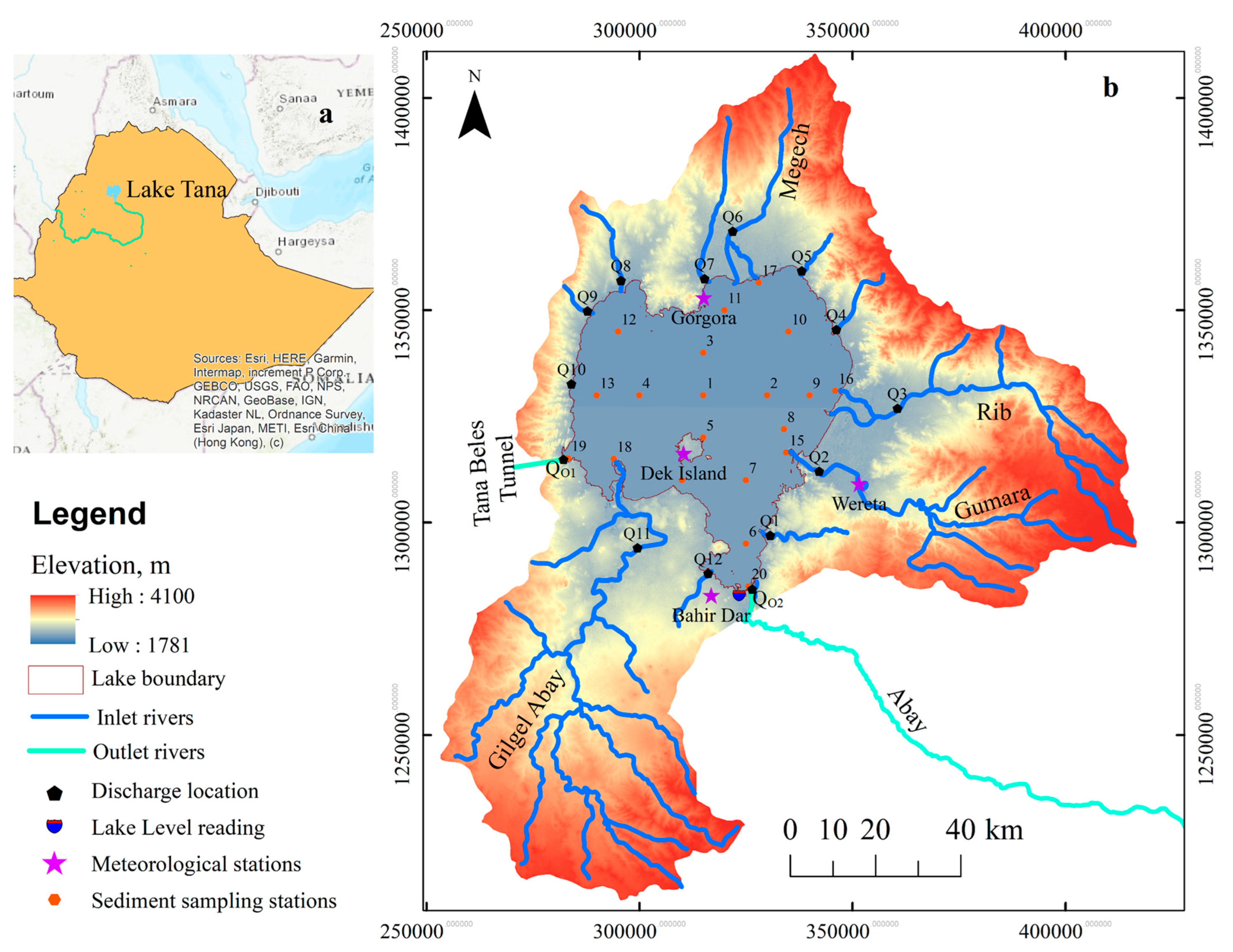
2.1. The Study Area

Lake Tana in the Blue Nile headwaters is in the northwestern highlands of Ethiopia (Figure 1). The lake has a nearly circular shape, a 3046 km2 surface area, and a volume of 29 km3 [49]. The lake is, on average, 10 m deep and the water mixes. Hence, vertical temperature gradient is not observed [31,49]. Lake Tana is the largest lake in Ethiopia [55]. It is a natural reservoir for Tana Beles and Tis Abay I and II hydropower plants [56]. The lake has great ecological importance. It is used for fishing, transportation, tourism, irrigation, and drinking. More than five hundred thousand people directly or indirectly depend on the lake and adjacent wetlands [55].
Water transparency in the lake is low due to large, suspended sediment loads [55] and resuspension from the lake bottom [26]. The average dissolved phosphorus concentration is 0.2 mg L−1 [19,57], and the available phosphorus is 19 mg P/kg in the bottom sediment [26]. The lake water quality is degraded [19,47]. Since 2011, water hyacinths have become a problem [40,58]. The water hyacinths in Lake Tana are concentrated in the northeast, with limited coverage on the eastern side [17,18,52].
More than 40 rivers feed the lake (Figure 1). The four largest rivers, Gilgel Abay, Gumara, Rib, and Megech, contribute around 90% of the flow and most sediment and nutrients to the lake [39,41,44]. Gilgel Abay, which covers 3900 km2 and enters the lake in the southwest, contributes about 60% of the inflow to the lake [42,59]. The Megech, joining the lake in the north, is the smallest of the four large rivers (Figure 1). The lake has two outlets: a natural outlet to the Abay (Blue Nile) on the south near Bahir Dar and an outlet to the Tana Beles hydropower plant on the western side [56]. Sediment concentrations in rivers entering the lake have increased [19,38,39]. Annually, about 40 Tg of sediment is lost from the uplands of the Lake Tana catchment [28,45]. Approximately 30% is deposited in the lake bed [46], and around 55% is deposited in the flood plains around the lake [45,46].

2.2. Data Collection

The meteorological data, inflow and outflow of Lake Tana, lake levels, suspended sediment concentrations, and the lake bathymetry used in this study are summarized in Figure A1 in Appendix A and presented in more detail below.

2.2.1. Meteorological Data

Precipitation, temperature, pan evaporation, hourly wind speed, and direction measurements were collected from the Bahir Dar, Dek Island, Gorgora, and Wereta stations from the Abay Basin Authority (Figure A1; station locations are given in Figure 1). The daily point rainfall was converted into areal rainfall using Theisen polygons (Figure S1, Supplementary Materials). Lake evaporation was calculated by multiplying the pan evaporation by 0.7 [60].

2.2.2. Inflow and Outflow Data

The 2017 river discharge data for the upper portion of the gauged rivers covering less than 50% of the basin were collected from the Ministry of Water and Energy (MWE). Discharge data for some of the smaller rivers entering Lake Tana for 2012 and 2013, labeled in Figure 1, were measured and published in Dessie et al. [42]. The discharge points are labeled Q1, Q2, Q3, Q6, Q9, and Q11 in Figure 1. The remainder of the discharge data for the ungauged part labeled Q4, Q5, Q7, Q8, Q10, and Q12 in Figure 1 were simulated by the Parameter-Efficient Distributed (PED) model [41,45]. The total 2017 inflow to the lake was determined by the sum of the discharge from the gauged and the ungauged rivers.
The 2017 outflow data through Abay was obtained from MWE (QO2). The outflow discharge through the Tana Beles Tunnel (QO1) is determined by dividing the power generation (provided by the Ethiopian Electric Power Authority by the generation efficiency, unit weight of water (9810 kg/m3) and the head difference between the lake level and the turbine (Figure A2 in Appendix A). The total lake outflow is then determined by adding the flows of the two outlets.

2.2.3. Lake Level and Bathymetry Data

Daily average lake level data (Figure A2) were obtained from the Abay Basin Authority. The observed lake level data was measured from a station in the southern part of Lake Tana (Figure 1). The bathymetric survey conducted in late 2017 was used for this study. The survey was performed on a 5 km grid and a round trip of the shore area. The data are published by Kebedew et al. [49].

2.2.4. Suspended Sediment Concentration Data

One-liter lake water samples were collected from 20 monitoring stations to determine the suspended sediment concentration during the rainfall phase in July, August, and September 2017 and in the dry phase in December 2017 and March 2018. The locations are depicted as numbers 1–20 in Figure 1. The sampling stations were close to the major inlet locations, which are the main sources of sediment and phosphorus: the central part of the lake, which is remote from transported material delivery; the southern region of the lake; the eastern and western portions of the lake; and near the mouth of the Blue Nile outlet and the offtake from the Tana-Beles hydroelectric power plant (Figure 1). A handheld GPS was used to find the sampling stations. The collected lake water samples were transported to the Bahir Dar Technology Institute water quality and treatment laboratory, Bahir Dar University, Ethiopia, for filtration. Water samples were filtered using Whatman filter paper with a pore size of 2.5 µm. The weight of sediment on the filter was determined after oven drying for 24 h at 105 °C.

2.3. Modeling Approach

2.3.1. Running the Model

The lake circulation pattern was simulated using the Delft3D-FLOW component of Delft3D model version 4.1. Delft3D is a state-of-the-art open-source modeling framework for lakes and reservoirs to simulate the hydrodynamics, water quality, ecology, waves, and morphology developed by Deltares in The Netherlands [61]. Delft3D-FLOW is a multi-dimensional (2D or 3D) hydrodynamic and transport simulation program that calculates non-steady hydrodynamic (and transport) phenomena in a curvilinear coordinate system [61]. It uses a continuity equation, a horizontal equation of motion, and a transport equation for conservative constituents. In Delft3D, the partial differential equations are transformed into discrete spaces and solved by the finite difference method.
The simulation of the flow pattern of Lake Tana consisted of delineating the lake boundary, grid generation, and defining physical and computational variables. As detailed in Kebedew et al. (2020) [49], the lake boundary was digitized from satellite image data. A total of 5600, 1-km2 square grid cells were generated within the lake boundary. Depth data for each grid was interpolated from the bathymetric survey using the existing reference level for lake level measurement, 1783.72 m a.s.l. [56].
Input data for the water balance computation of the model included the inflow to the lake at twelve points (Figure 1) and two outflow points (the Blue Nile and Tana Beles Tunnel). In addition, precipitation, evaporation, wind speed and direction, and hourly temperature were input parameters. Precipitation and evaporation are major water balance components because Lake Tana has a catchment area four times its size [41,42,44]. Finally, wind speed and direction play a major role in lake circulation and mixing [49].
Lake Tana has no thermal stratification and is fully mixed [31,49]. Hence, variations in sediment concentrations with depth could be ignored, and a two-dimensional simulation was employed for the analysis. The horizontal eddy viscosity and diffusivity were set to 0.002 m2 s−1 and 10 m2 s−1, according to the publication of Falconer et al. (1991) [62]. The Chezy coefficient value for bottom roughness was designated as a variable for calibration.
To evaluate the transport and distribution of suspended sediment and dissolved nutrients, a conservative tracer was released at the four major river outlets into the lake (Gilgel Abay, Gumara, Rib, and Megech) so that the river water had a concentration of 5 g L−1. The tracer release began in June at the same time the river discharge increased and continued until the end of August when the rains tapered off. See Figure 1 for locations of injections of the tracers in the four main rivers.
A ten-minute computational time step ensured computational stability during the simulation. The smoothing/startup time was 60 min for a smooth transition between the initial boundary condition and simulation [23]. The measured lake water level on 1 January 2017 was used as the initial water level for the simulation. The simulation was performed for one year (1 January to 31 December) with the 2017 metrological data. Inherently, it was assumed that the annual flows were cyclic. Simulated lake water level and tracer concentrations were recorded in text and graphical formats for each 10-min time step at the monitoring station labeled at the two outlets and the lake center to validate the lake water level (Stations 1, 19, and 20 in Figure 1).

2.3.2. Model Testing

The roughness coefficient was varied from 35 to 100 m0.5 to test its sensitivity to the lake-level simulations. To test the accuracy of the inflow–outflow data, the simulated lake levels were compared with the observed lake levels. Two simulations were performed. The first simulation used the observed data from MWE and Dessie et al. [42] as input. The second simulation used, in addition, inflow data simulated by PED [45] for the part of the basin that was not included in areas covered by MWE and [42].

2.3.3. Statistical Analysis

Organization of the data, conversion of the data from hourly to daily and monthly, and descriptive statistics, such as the mean, median, and standard deviation and root mean square error (RMSE), were determined. The spatial and temporal tracer distribution output and lake water level from the Delft3D model was also visualized. The suspended sediment distribution was mapped in ArcMap.

3. Results

3.1. Model Validation

For validation of the Delft3D model, the observed lake water levels were compared with the predicted water level. We found in the validation that the Root Mean Square Error (RSME) varied from 0.00395 to 0.00396 with a bottom roughness ranging from 35 to 100 m0.5. Thus, the effect of the bottom roughness was insignificant on the simulated lake water levels and the model default value for the bottom roughness of 65 m0.5 was adopted. In other publications, similar values were employed for large shallow lakes [23,35].
Rainfall, evaporation, inflow, and outflow are the parameters that affect the lake water level. The outflow and the meteorological data are more accurate than the inflow to the lake, especially when a sizable portion of the basin is ungauged. Therefore, the model performance depended greatly on the inflow from the ungauged areas (Figure 2). The simulated lake level with the available flow data from MWE and Dessie et al. [42] (dotted orange line) underpredicted the observed lake levels (Figure 2). Adding the discharge from the ungauged part, simulated by PED, the Delft3D model predicted the lake water level with an RSME of 0.00395 m (Figure 2).

3.2. Distribution of Observed Suspended Sediments of Lake Tana

Suspended sediment concentration (SSC), determined from 20 sampling locations on Lake Tana, had average concentrations of 99 mg/L in June, 300 mg/L in July, 352 mg/L in August, 222 mg/L in September, 142 mg/L in December, and 111 mg/L in March (Table 1). The SSC varies from a minimum of 13 mg/L in June at station 1 (lake center) to a maximum of 1926 mg/L in July at station 15 (near Gumara inlet). Secchi depth (Sec. dep) varied from 3 to 120 cm. The minimum was recorded at station 15 (close to the Gumara River inlet) in August, and the maximum was in March at the lake center at station 1 (Figure 1).
Spatially, during the rainy monsoon phase (July and August), the sediment concentrations were the most elevated, and the Secchi depths were the smallest at stations close to the major river inlets, namely 15, 16, 17, and 18. The stations at the center and northwest of the lake had the smallest concentrations and greatest light transparency (Figure 1 and Figure 3) for the locations of the stations. In addition, in the stretch from Megech to Gumara, the shallowest portion of the northeastern part of Lake Tana, the suspended sediment concentrations were elevated throughout the year (Figure 3). The statistics of the temporal values are summarized and presented in Table 1.
The resulting daily typical lake flow patterns are depicted in Figure 4. The main flow pattern is counterclockwise, especially when the wind comes from the southwest during the morning (Figure 4b). Near the east shore, the circulation is clockwise (Figure 4b–d). The clockwise flow pattern at night becomes larger, covering nearly half of the lake (Figure 4a). Near the southern shore, the outflow of the Gilgel Abay flows to the channel of the Tana Beles hydropower plant inlet and, to a lesser extent, to the Blue Nile outlet. In the northeast corner, the water of the Megech flows first to the east before joining the main clockwise loop. The wind direction changes cause several deviations in this main flow pattern, such as a reversal of the direction of the flow in the northeastern part of the lake during the afternoon and evening as a consequence of the northwest wind (Figure 4).

3.3. Tracer Distribution

Figure 5 shows the concentration of the tracer applied in the rain phase in the four main rivers from 1 June to 31 August. In Figure 5, all the tracer concentrations from the four main rivers are superimposed. The tracer distribution for the four individual rivers is depicted in Figure 6. The tracer concentration over time at the outlet and in the lake center is shown in Figure 7. The tracer concentrations indicate the general suspended sediment flow path, nutrient, and potential distribution when the sediment pickup from the bottom due to wave action and sediment deposition is not considered. Thus, the decrease in tracer concentration is due to the dilution.
When the tracers are released in June in the four main rivers, the tracer starts to distribute around the inlets (Figure 5 and Figure 6). In July, water and tracer from Gilgel Abay went directly to the Tana Beles hydroelectric plant channel to the east (Figure 6). In August, when the lake had risen and the outflow to the Blue Nile had increased, more flow and tracer went to the east and reached the Blue Nile outlet in September (Figure 6). In November, most of the tracer from the Gilgel Abay had gone away through both outlets. Some of the remaining tracers from the Gilgel Abay were transported northward near the east shore with a clockwise flow (Figure 4 and Figure 6). Also, some moved toward the lake center (Figure 6). The scenario before the operation of the Tana Beles Tunnel for hydropower generation in 1995 [56] was limited to the Abay outlet (Figure 7a).
Tracers from Gumara and Rib were initially distributed around the river inlets and then moved to the northeast with the counterclockwise flow depicted in Figure 4. The tracers covered a much smaller area than that of the Gilgel Abay because the discharge in each river was approximately one-third of Gilgel Abay (Figure 6). After the tracer application stopped and the discharge decreased at the end of August, the variable directions of the daily flows (Figure 4) dispersed the tracers over a wider area and consequently became less concentrated. A small amount of tracer from the Gumara found its way to the Blue Nile outlet in the middle of August (Figure 7b). The tracer released from the Megech River moved to the northeast of Lake Tana clockwise before joining the main counterclockwise flow (Figure 5 and Figure 6).
The distribution of the tracers released in the Gumara, Megech, and Rib overlap resulted in a greater tracer concentration in the northeastern part of the lake than for the individual rivers (Figure 5). The tracer released from the Gilgel Abay stayed mostly in the southern part of the lake. It did not overlap with the other rivers except near the mouth of the Blue Nile, with slightly greater tracer concentrations after August in Figure 5 than in Figure 6. In addition, all the rivers affected the tracer concentration in the center of the Lake (Figure 5, Figure 6 and Figure 7c).

4. Discussion

4.1. The Flow Pattern of Lake Tana

The simulated flow and tracer concentration patterns of Lake Tana provide information on the distribution and dynamics of sediment and nutrients. Comparing the tracer concentration (Figure 5) with that of the suspended sediment concentration (SSC) and the Secchi desk depth (Figure 3), a similar pattern emerges, even though the tracer concentrations were not subject to deposition, unlike the suspended solids. In the southern half of the lake, the flow pattern was dominated by the inflow of the Gilgel Abay, the outflow to the Tunnel of the Tana Beles hydropower station, and the outflow to the Abay (Blue Nile) in both the tracer and SSC concentrations and Secchi depth (Figure 3 and Figure 5). When the discharge was small in June, the slightly elevated concentrations and reduced Secchi depth were just around the Gilgel Abay outlet. In July, when the discharge was greater, the concentration increased and could be seen over an extended area. In August and September, with the high discharge of the Gilgel Abay, it grew further, and then the tracer reached the Blue Nile. The distribution was similar to the Sechi depth reduction but was not as obvious in the SSC concentration distribution in Figure 3. In December, most of the tracer and sediment were lost in the two outlets resulting in lower concentrations and increased Secchi depth readings (Figure 3 and Figure 5).
The tracer and suspended sediment patterns in the north and east of the lake were mainly affected by the counterclockwise flow pattern (Figure 4 and Figure 5). The counterclockwise flow moved the sediment and tracer of the Gumara and Rib northward, increasing its area from June to September. Especially in August, more suspended solids were flowing from the Gumara than indicated by the tracer distribution. In December, the overall tracer concentration in the lake varied from 0.4 to 0.8 g L−1 (Figure 5), which is 8 to 16% of the tracer concentration in the river from June to August. The sediment concentrations ranged from 50 to 300 mg L−1 in December. That is around 3–20% of the maximum concentration of 1500 mg L−1. Despite the sediment being deposited on the bottom of the lake, tracer and sediment concentrations are in the same range, indicating that dilution and loss through the outlets also play a role in the suspended concentrations.

4.2. Implication on Sediment and Nutrient Dynamics of Lake Tana

The flow pattern of Lake Tana plays a critical role in distributing the suspended sediment and nutrients in the lake. Due to the circulation pattern induced by the river discharge, water, sediment, and nutrients, such as phosphorus delivered by the Gilgel Abay River to the lake, flow to the two outlets (Abay and Tana Beles Tunnel) and are discharged from the lake relatively quickly. In contrast, the water, sediment, and nutrients from the Gumara and Rib Rivers from the east are transported to the northeast of Lake Tana following the counterclockwise flow pattern (Figure 4 and Figure 6). The flow from the Megech in the north flows to the east with a clockwise pattern to the northeast.
Consequently, most of the water and sediment delivered from the eastern and northern catchments stay longer in Lake Tana than the flow originating from the much larger Gilgel Abay. Due to the long retention time, water is lost by evaporation. The annual evaporation rate in Lake Tana is nearly 20% of the lake volume [49]. Therefore, sediment and phosphorus are retained because when the water evaporates, it cannot carry and sediment and phosphorus to the outlets.
Due to the accumulation of sediment and phosphorus from the northern and eastern catchments, the northeast of Lake Tana has the greatest suspended sediment and the shortest Secchi disk depth (Figure 2). The deposited sediments and phosphorus recycle back in the water column later in the dry season, when the lake water level is reduced [18,19,26] and causes elevated dissolved phosphorus concentrations in the northeast in the dry season [49]. Further research is also important through the water quality component of the Delft3D model to investigate the effect of the circulation pattern on specific water quality parameters.

4.3. Distribution of Water Hyacinth in Lake Tana

The spread of water hyacinth in Lake Tana is dynamic but limited to the northeast and partly to the east of the lake [18,50,52]. The suspended sediments and the available phosphorus from the Gumara, Rib, and Megech accumulate in the northeastern part of the lake (Figure 4 and Figure 5). The greatest sediment and available phosphorus concentration is thus in the northeast, where it reaches up to 38.5 mg P/kg while the average is 19 mg P/kg [26]. The phosphorus in the lake sediment is in equilibrium with the phosphorus dissolved in the lake water [63]. Therefore, dissolved phosphorus is also the highest in the northeastern part of the lake, with a maximum value of 0.6 mg P/L, which is about three times the average value of the lake at 0.21 mg P/L [19,26]. The main nutrient for the growth of water hyacinth is phosphorus [12]. Thus, the greatest expansion of the water hyacinths is on the northeastern side of Lake Tana. On the western side, the sediment and nutrients from Gilgel Abay flow out of Lake Tana through the Tana Beles outlets close to the Gilgel Abay River inlet (Figure 1, Figure 5 and Figure 6). As a result, the growth of water hyacinth is less likely on the western and southwestern sides of the lake.
Water hyacinth floats, grows rapidly, and can spread via lake currents [37]. Therefore, the accumulation of water hyacinth in the northeast of Lake Tana is due to the counterclockwise rotation of sediments from the Gumara and Rib, and the clockwise rotation of a portion of the sediments from the Gilgel Abay and all the sediments from the Megech (Figure 3). In the northeast, the flow pattern intersects, thus accumulating the water hyacinth near that area (Figure 4). In addition, the circulation in the west is away from the shore (Figure 3), while in the east and northeast, the flow patterns are towards the shore, preventing the water hyacinth from moving back to the center and other locations (Figure 3). Thus, the lake current hinders it from spreading back to the different areas of the lake. The accumulated suspended sediment and phosphorus in the northeast are generated from the northern and eastern catchments. Hence, control management strategies for water hyacinths should focus on reducing sediment and phosphorus concentrations in the catchments of north and east Lake Tana.

5. Conclusions

The paper addressed the effect of lake circulation on sediment and nutrient distribution and its implications on the spread of the water hyacinths in Lake Tana. The Delft3D-FLOW model was developed and applied to investigate the sediment and nutrient distribution and transport paths of Lake Tana. To visualize the transport of suspended sediment and dissolved nutrients on Lake Tana, inert tracers were released through the four main rivers draining into the lake. The performance of the model was assessed by comparing the observed and predicted lake water levels. The result showed that the lake circulation was counterclockwise except in the eastern part of Lake Tana. The counterclockwise flow pattern from the north and clockwise from the east intersects in the northeast and then recirculates back to lake outlet locations. Hence, the water, sediment, and associated nutrients, such as phosphorus generated from the eastern and northern catchments, had the longest retention time in the northeast of Lake Tana. As a result, most of the water is lost through evaporation while the sediment and phosphorus are partly suspended in the area and absorbed in the lakebed in the northeast. Therefore, the accumulated phosphorus creates a favorable condition for the growth of water hyacinths in the location. Whereas the sediments and nutrients delivered from Gilgel Abay, southwest of Lake Tana, flow out of the lake through the two outlets in a shorter retention time favored by the close locations with the outlets. Thus, the northeast of Lake Tana is a preferable site for water hyacinth growth due to its greatest suspended sediment and phosphorus concentration. Moreover, the spread of water hyacinth is limited to the northeast of Lake Tana due to the counterclockwise flow from the north and clockwise flow from the east which prevents it from spreading to other locations. Hence, the management and control mechanisms for water hyacinths should be focused on reducing sediment and phosphorus concentrations from the northern and eastern catchment areas of Lake Tana. Further study is recommended to identify hotspot areas for the runoff, sediment, and nutrient concentrations of the lake watershed, which could help to limit the spread of water hyacinths in Lake Tana.

Supplementary Materials

The following supporting information can be downloaded at: https://www.mdpi.com/article/10.3390/hydrology10090181/s1, Figure S1: Theisen polygon for calculating precipitation on Lake Tana.

Author Contributions

M.G.K. has contributed to conceptualization, data collection, data analysis, writing the original draft manuscript, and improving the manuscript based on the comments and suggestions of the co-authors. S.A.T. aided in formulating the objectives, administered the project, supervised, reviewed, and edited. M.A.B. contributed to formulating the methods and reviewing and editing the draft, F.A.Z. provided comments and suggestions on the research and paper drafts. M.D.W. contributed to the flow of data, and T.S.S. contributed to the conceptualization, overall content, and structure of the paper, supervising, and improving the English. All authors have read and agreed to the published version of the manuscript.

Funding

The research was funded by the EXCEED–SWINDON project “Excellence Center for Development Cooperation–Sustainable Water Management in Developing Countries” centered in the Technical University of Braunschweig, Germany (http://www.exceed-swindon.org, accessed on 25 December 2021) within the framework of the DAAD Programme, and Blue Nile Water Institute of Bahir Dar University, Ethiopia. Additional funding was provided by the Robert S. McNamara Fellowships Program of the World Bank and an anonymous donor through Cornell University.

Data Availability Statement

Data that are not owned by the Ethiopian Government can be requested from the author.

Acknowledgments

We would like to acknowledge the assistance of Getahun Birra during the water sample collection and Mahder Anteneh during the suspended sediment filtration. We acknowledge the assistance of Nick van de Giesen, Water Resources Management, TU Delft, and Kees Sloff, Menno Genseberger, and Pascal Boderie, Deltares, The Netherlands, to the first author during his stay in The Netherlands. We thank the Abay Basin Authority for providing the metrological data and the Ministry of Water and Energy for the flow data.

Conflicts of Interest

The authors declare no conflict of interest.

Appendix A

Figure A1. Water balance components of Lake Tana: the monthly volume of water for each component. Precipitation = total annual rainfall at the lake surface area; Evaporation = annual Lake surface evaporation; Inflow = total inflow to the lake (all flows through the gauged rivers and all flows through the ungauged rivers or tributaries; Outflow = total outflow from the lake (outflow through Blue Nile River and outflow through the Tana Beles Tunnel that diverts water for hydroelectric power generation).
Hydrology 10 00181 g0a1
Figure A2. Lake outflow through Tana Beles and Blue Nile outlet and Lake Water Level of Lake Tana in 2017 (See Figure 1 for the outflow measurement locations and lake level measurement station).
Hydrology 10 00181 g0a2

References

  1. Tsanis, I.K. Environmental Hydraulics: Hydrodynamic and Pollutant Transport Modeling of Lakes and Coastal Waters; Elsevier: Amsterdam, The Netherlands, 2006. [Google Scholar]
  2. Bhateria, R.; Jain, D. Water quality assessment of lake water: A review. Sustain. Water Resour. Manag. 2016, 2, 161–173. [Google Scholar] [CrossRef]
  3. Fink, G.; Alcamo, J.; Flörke, M.; Reder, K. Phosphorus loadings to the world’s largest lakes: Sources and trends. Glob. Biogeochem. Cycles 2018, 32, 617–634. [Google Scholar] [CrossRef]
  4. Sheela, A.M.; Letha, J.; Joseph, S.; Ramachandran, K.K.; Sanalkumar, S. Trophic state index of a lake system using IRS (P6-LISS III) satellite imagery. Environ. Monit. Assess. 2011, 177, 575–592. [Google Scholar] [CrossRef] [PubMed]
  5. Syvitski, J.P.; Vörösmarty, C.J.; Kettner, A.J.; Green, P. Impact of humans on the flux of terrestrial sediment to the global coastal ocean. Science 2005, 308, 376–380. [Google Scholar] [CrossRef] [PubMed]
  6. Bingxue, H. Eutrophication Assessment in Songbei Wetlands: A Comparative Methods. In Computing and Intelligent Systems, Proceedings of the International Conference, ICCIC 2011, Wuhan, China, 17–18 September 2011; Proceedings, Part IV; Springer: Berlin/Heidelberg, Germany, 2011. [Google Scholar]
  7. Aktar, M.W.; Sengupta, D.; Chowdhury, A. Impact of pesticides use in agriculture: Their benefits and hazards. Interdiscip. Toxicol. 2009, 2, 1. [Google Scholar] [CrossRef] [PubMed]
  8. Larson, B.A.; Frisvold, G.B. Fertilizers to support agricultural development in sub-Saharan Africa: What is needed and why. Food Policy 1996, 21, 509–525. [Google Scholar] [CrossRef]
  9. Olsen, R. Effects of intensive fertilizer use on the human environment: A summary review. FAO Soils Bull. 1978, 116, 15–33. [Google Scholar]
  10. Konstantinou, I.K.; Hela, D.G.; Albanis, T.A. The status of pesticide pollution in surface waters (rivers and lakes) of Greece. Part I. Review on occurrence and levels. Environ. Pollut. 2006, 141, 555–570. [Google Scholar] [CrossRef]
  11. Rask, M.; Olin, M.; Ruuhijärvi, J. Fish-based assessment of ecological status of Finnish lakes loaded by diffuse nutrient pollution from agriculture. Fish. Manag. Ecol. 2010, 17, 126–133. [Google Scholar] [CrossRef]
  12. Kobayashi, J.T.; Thomaz, S.M.; Pelicice, F.M. Phosphorus as a limiting factor for Eichhornia crassipes growth in the upper Paraná River floodplain. Wetlands 2008, 28, 905–913. [Google Scholar] [CrossRef]
  13. Wang, J.; Zhao, Q.; Pang, Y.; Hu, K. Research on nutrient pollution load in Lake Taihu, China. Environ. Sci. Pollut. Res. 2017, 24, 17829–17838. [Google Scholar] [CrossRef]
  14. Phiri, G.; Navarro, L. Water Hyacinth in Africa and the Middle East: A Survey of Problems and Solutions; International Development Research Centre: Ottawa, ON, Canada, 2000. [Google Scholar]
  15. Odada, E.O.; Olago, D.O.; Olaka, L.A. An East African perspective of the Anthropocene. Sci. Afr. 2020, 10, e00553. [Google Scholar] [CrossRef]
  16. Dersseh, M.G.; Melesse, A.M.; Tilahun, S.A.; Abate, M.; Dagnew, D.C. Water hyacinth: Review of its impacts on hydrology and ecosystem services—Lessons for management of Lake Tana. In Extreme Hydrology and Climate Variability; Elsevier: Amsterdam, The Netherlands, 2019; pp. 237–251. [Google Scholar]
  17. Asmare, G.; Abate, M. Morphological changes in the lower reach of Megech River, Lake Tana basin, Ethiopia. In Advances of Science and Technology, Proceedings of the 6th EAI International Conference, ICAST 2018, Bahir Dar, Ethiopia, 5–7 October 2018; Proceedings 6; Springer: Berlin/Heidelberg, Germany, 2019; pp. 32–49. [Google Scholar]
  18. Dersseh, M.G.; Tilahun, S.A.; Worqlul, A.W.; Moges, M.A.; Abebe, W.B.; Mhiret, D.A.; Melesse, A.M. Spatial and temporal dynamics of water hyacinth and its linkage with lake-level fluctuation: Lake Tana, a sub-humid region of the Ethiopian highlands. Water 2020, 12, 1435. [Google Scholar] [CrossRef]
  19. Dersseh, M.G.; Steenhuis, T.S.; Kibret, A.A.; Eneyew, B.M.; Kebedew, M.G.; Zimale, F.A.; Worqlul, A.W.; Moges, M.A.; Abebe, W.B.; Mhiret, D.A. Water quality characteristics of a water hyacinth infested tropical highland lake: Lake Tana, Ethiopia. Front. Water 2022, 4, 774710. [Google Scholar] [CrossRef]
  20. Kaba, E.; Philpot, W.; Steenhuis, T. Evaluating suitability of MODIS-Terra images for reproducing historic sediment concentrations in water bodies: Lake Tana, Ethiopia. Int. J. Appl. Earth Obs. Geoinf. 2014, 26, 286–297. [Google Scholar] [CrossRef]
  21. Siev, S.; Yang, H.; Sok, T.; Uk, S.; Song, L.; Kodikara, D.; Oeurng, C.; Hul, S.; Yoshimura, C. Sediment dynamics in a large shallow lake characterized by seasonal flood pulse in Southeast Asia. Sci. Total Environ. 2018, 631, 597–607. [Google Scholar] [CrossRef]
  22. Zhang, W.; Xu, Q.; Wang, X.; Hu, X.; Wang, C.; Pang, Y.; Hu, Y.; Zhao, Y.; Zhao, X. Spatiotemporal distribution of eutrophication in Lake Tai as affected by wind. Water 2017, 9, 200. [Google Scholar] [CrossRef]
  23. Liu, S.; Ye, Q.; Wu, S.; Stive, M.J. Horizontal circulation patterns in a large shallow lake: Taihu Lake, China. Water 2018, 10, 792. [Google Scholar] [CrossRef]
  24. You, B.-S.; Zhong, J.-C.; Fan, C.-X.; Wang, T.-C.; Zhang, L.; Ding, S.-M. Effects of hydrodynamics processes on phosphorus fluxes from sediment in large, shallow Taihu Lake. J. Environ. Sci. 2007, 19, 1055–1060. [Google Scholar] [CrossRef]
  25. Blottiere, L. The Effects of Wind-Induced Mixing on the Structure and Functioning of Shallow Freshwater Lakes in a Context of Global Change; Université Paris Saclay (COmUE): Paris, France, 2015. [Google Scholar]
  26. Kebedew, M.G.; Tilahun, S.A.; Zimale, F.A.; Steenhuis, T.S. Bottom sediment characteristics of a tropical lake: Lake Tana, Ethiopia. Hydrology 2020, 7, 18. [Google Scholar] [CrossRef]
  27. Scheffer, M. Ecology of Shallow Lakes; Kluwer Academic Publishers: Dordrecht, The Netherlands, 2004. [Google Scholar]
  28. Lemma, H.; Admasu, T.; Dessie, M.; Fentie, D.; Deckers, J.; Frankl, A.; Poesen, J.; Adgo, E.; Nyssen, J. Revisiting lake sediment budgets: How the calculation of lake lifetime is strongly data and method dependent. Earth Surf. Process. Landf. 2018, 43, 593–607. [Google Scholar] [CrossRef]
  29. Aga, A.O.; Melesse, A.M.; Chane, B. Estimating the sediment flux and budget for a data limited rift valley lake in Ethiopia. Hydrology 2018, 6, 1. [Google Scholar] [CrossRef]
  30. Xu, M.; Dong, X.; Yang, X.; Chen, X.; Zhang, Q.; Liu, Q.; Wang, R.; Yao, M.; Davidson, T.A.; Jeppesen, E. Recent sedimentation rates of shallow lakes in the middle and lower reaches of the Yangtze River: Patterns, controlling factors and implications for lake management. Water 2017, 9, 617. [Google Scholar] [CrossRef]
  31. Dargahi, B.; Setegn, S.G. Combined 3D hydrodynamic and watershed modelling of Lake Tana, Ethiopia. J. Hydrol. 2011, 398, 44–64. [Google Scholar] [CrossRef]
  32. Ssebuggwawo, V.; Kitamirike, J.; Khisa, P.; Njuguna, H.; Myanza, O.; Hecky, R.; Mwanuzi, F. Hydraulic/Hydrodynamic Conditions of Lake Victoria; Lake Victoria Environmental Management Project (LVEMP): Entebbe, Uganda, 2005. [Google Scholar]
  33. Ndungu, J.N.; Chen, W.; Augustijn, D.C.; Hulscher, S.J. Analysis of the driving force of hydrodynamics in Lake Naivasha, Kenya. Open J. Mod. Hydrol. 2015, 5, 95–104. [Google Scholar] [CrossRef]
  34. El-Arab, N.B. Coupled hydrodynamic-water quality model for pollution control scenarios in El-Burullus Lake (Nile delta, Egypt). Austrian J. Earth Sci. 2014, 8, 53. [Google Scholar]
  35. Ouni, H.; Sousa, M.; Ribeiro, A.; Pinheiro, J.; M’Barek, N.B.; Tarhouni, J.; Tlatli-Hariga, N.; Dias, J. Numerical modeling of hydrodynamic circulation in Ichkeul Lake-Tunisia. Energy Rep. 2020, 6, 208–213. [Google Scholar] [CrossRef]
  36. Razmi, A.M.; Barry, D.A.; Bakhtyar, R.; Le Dantec, N.; Dastgheib, A.; Lemmin, U.; Wüest, A. Current variability in a wide and open lacustrine embayment in Lake Geneva (Switzerland). J. Great Lakes Res. 2013, 39, 455–465. [Google Scholar] [CrossRef]
  37. Vijverberg, T.; Winterwerp, J.C.; Aarninkhof, S.G.J.; Drost, H. Fine sediment dynamics in a shallow lake and implication for design of hydraulic works. Ocean Dyn. 2011, 61, 187–202. [Google Scholar] [CrossRef]
  38. Abate, M.; Nyssen, J.; Moges, M.M.; Enku, T.; Zimale, F.A.; Tilahun, S.A.; Adgo, E.; Steenhuis, T.S. Long-term landscape changes in the Lake Tana Basin as evidenced by delta development and floodplain aggradation in Ethiopia. Land Degrad. Dev. 2017, 28, 1820–1830. [Google Scholar] [CrossRef]
  39. Alemu, M.L.; Geset, M.; Mosa, H.M.; Zemale, F.A.; Moges, M.A.; Giri, S.K.; Tillahun, S.A.; Melesse, A.M.; Ayana, E.K.; Steenhuis, T.S. Spatial and temporal trends of recent dissolved phosphorus concentrations in Lake Tana and its four main tributaries. Land Degrad. Dev. 2017, 28, 1742–1751. [Google Scholar] [CrossRef]
  40. Gezie, A.; Assefa, W.W.; Getnet, B.; Anteneh, W.; Dejen, E.; Mereta, S.T. Potential impacts of water hyacinth invasion and management on water quality and human health in Lake Tana watershed, Northwest Ethiopia. Biol. Invasions 2018, 20, 2517–2534. [Google Scholar] [CrossRef]
  41. Alemu, M.L.; Worqlul, A.W.; Zimale, F.A.; Tilahun, S.A.; Steenhuis, T.S. Water balance for a tropical lake in the volcanic highlands: Lake Tana, Ethiopia. Water 2020, 12, 2737. [Google Scholar] [CrossRef]
  42. Dessie, M.; Verhoest, N.E.; Pauwels, V.R.N.; Admasu, T.; Poesen, J.; Adgo, E.; Deckers, J.; Nyssen, J. Analyzing runoff processes through conceptual hydrological modeling in the Upper Blue Nile Basin, Ethiopia. Hydrol. Earth Syst. Sci. 2014, 18, 5149–5167. [Google Scholar] [CrossRef]
  43. Chebud, Y.A.; Melesse, A.M. Modelling lake stage and water balance of Lake Tana, Ethiopia. Hydrol. Process. Int. J. 2009, 23, 3534–3544. [Google Scholar] [CrossRef]
  44. Kebede, S.; Travi, Y.; Alemayehu, T.; Marc, V. Water balance of Lake Tana and its sensitivity to fluctuations in rainfall, Blue Nile basin, Ethiopia. J. Hydrol. 2006, 316, 233–247. [Google Scholar] [CrossRef]
  45. Zimale, F.A.; Moges, M.A.; Alemu, M.L.; Ayana, E.K.; Demissie, S.S.; Tilahun, S.A.; Steenhuis, T.S. Budgeting suspended sediment fluxes in tropical monsoonal watersheds with limited data: The Lake Tana basin. J. Hydrol. Hydromech. 2018, 66, 65–78. [Google Scholar] [CrossRef]
  46. Kebedew, M.G.; Tilahun, S.A.; Belete, M.A.; Zimale, F.A.; Steenhuis, T.S. Sediment deposition (1940–2017) in a historically pristine lake in a rapidly developing tropical highland region in Ethiopia. Earth Surf. Process. Landf. 2021, 46, 1521–1535. [Google Scholar] [CrossRef]
  47. Goshu, G.; Koelmans, A.; de Klein, J. Water quality of Lake Tana basin, Upper Blue Nile, Ethiopia. A review of available data. In Social and Ecological System Dynamics: Characteristics, Trends, and Integration in the Lake Tana Basin, Ethiopia; Springer: Berlin/Heidelberg, Germany, 2017; pp. 127–141. [Google Scholar]
  48. Wondie, A.; Mengistu, S.; Vijverberg, J.; Dejen, E. Seasonal variation in primary production of a large high altitude tropical lake (Lake Tana, Ethiopia): Effects of nutrient availability and water transparency. Aquat. Ecol. 2007, 41, 195–207. [Google Scholar] [CrossRef]
  49. Kebedew, M.G.; Kibret, A.A.; Tilahun, S.A.; Belete, M.A.; Zimale, F.A.; Steenhuis, T.S. The relationship of lake morphometry and phosphorus dynamics of a tropical Highland Lake: Lake Tana, Ethiopia. Water 2020, 12, 2243. [Google Scholar] [CrossRef]
  50. Asmare, T.; Demissie, B.; Nigusse, A.G.; GebreKidan, A. Detecting spatiotemporal expansion of water hyacinth (Eichhornia crassipes) in Lake Tana, Northern Ethiopia. J. Indian Soc. Remote Sens. 2020, 48, 751–764. [Google Scholar] [CrossRef]
  51. Tewabe, D. Preliminary survey of water hyacinth in Lake Tana, Ethiopia. Glob. J. Allergy 2015, 1, 013–018. [Google Scholar] [CrossRef]
  52. Worqlul, A.W.; Ayana, E.K.; Dile, Y.T.; Moges, M.A.; Dersseh, M.G.; Tegegne, G.; Kibret, S. Spatiotemporal dynamics and environmental controlling factors of the Lake Tana water hyacinth in Ethiopia. Remote Sens. 2020, 12, 2706. [Google Scholar] [CrossRef]
  53. Admas, A.; Sahile, S.; Agidie, A.; Menale, H.; Gedefaw, T.; Teshome, M. Controlling water hyacinth infestation in Lake Tana using Fungal pathogen from Laboratory level upto pilot scale. bioRxiv 2020. [Google Scholar] [CrossRef]
  54. Wondim, Y.K.; Mosa, H.M. Spatial variation of sediment physicochemical characteristics of Lake Tana, Ethiopia. J. Environ. Earth Sci. 2015, 5, 95–109. [Google Scholar]
  55. Vijverberg, J.; Sibbing, F.A.; Dejen, E. Lake Tana: Source of the blue nile. In The Nile: Origin, Environments, Limnology and Human Use; Springer: Berlin/Heidelberg, Germany, 2009; pp. 163–192. [Google Scholar]
  56. McCartney, M.; Alemayehu, T.; Shiferaw, A.; Awulachew, S. Evaluation of Current and Future Water Resources Development in the Lake Tana Basin, Ethiopia; IWMI: Colombo, Sri Lanka, 2010; Volume 134. [Google Scholar]
  57. Ethiopia, T. Water Quality Assessment by Measuring and Using Landsat 7 ETM+ Images for the Current and Previous Trend Perspective: Lake. J. Water Resour. Prot. 2017, 9, 1564–1585. [Google Scholar]
  58. Anteneh, W.; Dereje, T.; Addisalem, A.; Abebaw, Z.; Befta, T. Water Hyacinth Coverage Survey Report on Lake Tana; Bahir Dar University: Bahir Dar, Ethiopia, 2015. [Google Scholar]
  59. IP SMEC. Hydrological study of the Tana-Beles sub-basins. In Surface Water Investigation; MOWR: Addis Ababa, Ethiopia, 2007. [Google Scholar]
  60. Stanhill, G. The CIMO International Evaporimeter Comparisons; Secretariat of the WMO: Geneva, Switzerland, 1976. [Google Scholar]
  61. Manual, D. 3D/2D Modelling Suite for Integral Water Solutions; Deltares: Delft, The Netherlands, 2014. [Google Scholar]
  62. Falconer, R.; George, D.; Hall, P. Three-dimensional numerical modelling of wind-driven circulation in a shallow homogeneous lake. J. Hydrol. 1991, 124, 59–79. [Google Scholar] [CrossRef]
  63. Wu, Y.; Wen, Y.; Zhou, J.; Wu, Y. Phosphorus release from lake sediments: Effects of pH, temperature and dissolved oxygen. KSCE J. Civ. Eng. 2014, 18, 323–329. [Google Scholar] [CrossRef]
Figure 1. Location of the study area: (a) map of Lake Tana and Ethiopia in the National Geographic World Map and (b) Lake Tana basin indicating sampling points for suspended sediment, inflow and outflow points, and locations for lake level measurement and meteorological stations at Q1, Q2, Q3, Q6, Q9, and Q11.
Hydrology 10 00181 g001
Figure 2. Comparison of observed and simulated 2017 lake levels. “Predicted WL 2” (dashed blue line) is the simulated water level using the discharge of the upper Lake Tana basin and outflow data of the Ministry of Water and Energy, the Tana Beles hydroelectric power station outflow, and inflow data of the lower portion partly observed by Dessie et al. [42] and partially simulated by Parameter Efficient Distribution Model [45]. Predicted WL 1 (dotted orange line) is the water level with the observed river discharge data but without the simulated flows.
Hydrology 10 00181 g002
Figure 3. Spatial and temporal distribution of suspended sediment concentration (SSC, mg/L) and Secchi disk depth (Sec. dep, cm) of Lake Tana collected from 20 monitoring stations from June 2017 to March 2018. (See Figure 1 for the location of the sampling stations).
Hydrology 10 00181 g003
Figure 4. Diurnal variations of flow patterns and depth-averaged velocity of Lake Tana, the maps retrieved from the model for 3 July 2017 (a) late at night; (b) morning; (c) afternoon; and (d) evening.
Hydrology 10 00181 g004
Figure 5. Monthly maps of tracer distribution in Lake Tana after the tracers were released in June through the four major inlet rivers flowing in the lake (Gilgel Abay, Gumara, Rib, and Megech). Spatial maps are retrieved at 9:00 a.m. on the 5th day of the month. The trace application was stopped on 31 August.
Hydrology 10 00181 g005
Figure 6. Time series tracer distribution of Lake Tana, when the tracers are released individually through the four major rivers inlets from 1 June to 31 August. Maps are retrieved at 9:00 a.m. on the 5th day of each month from June to December.
Hydrology 10 00181 g006
Figure 7. Tracer concentration plots at observation points released through Gilgel Abay, Gumara, Rib, and Megech inlets of Lake Tana from 1 June to 31 August (a) concentration of tracer outflow at the two outlets (b) at Abay (Blue Nile) outlet (c) at the center of the lake.
Hydrology 10 00181 g007
Table 1. Summary of suspended sediment concentration (SSC) and Secchi disk depth in Lake Tana from June 2017 to March 2018.
JuneJulyAugustSeptemberDecemberMarch
SSC, mg L−1Maximum28019261567567372287
Minimum131316924422
Mean99300352222142111
St. deviation9452447716110183
Secchi depth, cmMaximum9495704891120
Minimum1553104638
Mean494330306982
St. deviation23.329.119.611.014.229.2
Disclaimer/Publisher’s Note: The statements, opinions and data contained in all publications are solely those of the individual author(s) and contributor(s) and not of MDPI and/or the editor(s). MDPI and/or the editor(s) disclaim responsibility for any injury to people or property resulting from any ideas, methods, instructions or products referred to in the content.

