Effects of a Gravel Pit Lake on Groundwater Hydrodynamic

Abstract

In Europe, 1132 Mt of sand and gravel were mined in 2019, which causes major changes to the hydrogeological cycle. Such changes may lead to significantly raised or lowered groundwater levels. Therefore, the aggregate sector has to ensure that impacts on existing environmental and water infrastructures are kept to a minimum in the post-mining phase. Such risk assessments are often made by empirical methods, which are based on assumptions that do not meet real aquifer conditions. To investigate this effect, predictions by empirical and numerical methods about hydraulic head changes caused by a pit lake were compared. Wrobel’s equation, which is based on Sichardt’s equation, was used as the empirical method, while a numerical groundwater flow model has been solved by means of the finite-element method in FEFLOW. The empirical method provides significantly smaller ranges of increased/decreased groundwater levels caused by the gravel pit lake as the numerical method. The underestimation of the empirical results was related to the finding that field measurements during pumping tests show a larger extent of groundwater drawdown than calculations with the Sichardt’s equation. Simplifications of the 2D model approach have been evaluated against hydraulic head changes derived from a 3D groundwater model. Our results clearly show that the faster and cheaper empirical method—Wrobel’s equation, which is often preferred over the more expensive and time-consuming numerical method, underestimates the drawdown area. This is especially critical when the assignment of mining permits is based on such computations. Therefore, we recommend using numerical models in the pre-mining phase to accurately compute the extent of a gravel/sand excavation’s impacts on hydraulic head and hence more effective protection of groundwater and other related environmental systems.

1. Introduction

The aggregate industry, including extraction of gravel and sand from fluvial deposits by open-pit mechanical extraction, as well as from lakes, rivers, and sea by dredging, plays a key role in European’s economy by providing materials for the construction sector [1,2,3]. European countries (EU-28) extracted even 1132 Mt of sand and gravel in 2019 [4].

A gravel pit lake (pit lake), which is the subject of this paper, remains as the final landform of the open-pit gravel mining. On one hand, pit lakes may present environmental risks, including a risk to drinking water supplies; on the other hand, they have the potential to become a beneficial end-use resource [5]. Groundwater flow through pit lakes, which can be called flow-through lakes [6], leads to significant impacts on the environment such as morphological changes, changes of (bio)chemical cycles in lake water and groundwater [7], changes in groundwater quality due to air- and water-born contaminants [8,9], harming existing terrestrial areas [10], creating valuable freshwater ecosystems [10], groundwater warming due to its exposure to air temperature [5], increased freshwater loss due to faster evaporation from the surface water, and slower evapotranspiration in a vegetated land [7], among others.

Changes in the hydrogeological cycle can cause raising or lowering of groundwater levels that lead to deteriorated conditions for farmers, water suppliers, groundwater-dependent ecosystems, or other groundwater-dependent sectors. A pit lake leads to a drawdown and mounding that occur up-gradient and down-gradient from a pit lake, respectively [11]. Thus, before the excavation (pre-mining phase), mining companies have to provide the expected impacts of the pit lake on local and regional hydrogeology. For such purposes, hydrogeologists use methods such as simple empirical equations, complex analytical solutions, or numerical methods [12].

Different empirical and numerical methods, with their specific advantages and uncertainties due to their limitations, deliver non-uniform results. Empirical solutions in hydrogeology often assume a homogeneous and isotropic hydraulic conductivity distribution, horizontal flow (and thus a horizontal aquifer bottom), infinite horizontal extent, and limited boundary conditions [13]. Such approximations of the real world make it difficult or even impossible to obtain reliable results based on empirical approaches to calculate groundwater drawdown and mounding by pit lakes. However, empirical approaches are still often used due to a lack of resources and/or measurement datasets in engineering practice.

As an alternative, numerical methods provide a non-unique solution for more complex systems, which is based on the understanding of a problem being solved [14,15] (p. 78). In studies of physical phenomena, partial-differential equations (e.g., groundwater flow equation) can be solved with different numerical approximations. In this way, a complex problem, such as transient groundwater flow under a heterogeneous or anisotropic hydraulic conductivity distribution, multiple boundary conditions and a diverse elevation of the model’s base can be defined [13]. Several software packages are available for solving numerical methods in hydrogeology. In this paper, FEFLOW from MIKE Powered by DHI is applied, in which the Finite-Element Method (FEM) is implemented.

A concern about potential conflicts among mining companies, stakeholders, and society due to inconsistent assessments of a pit lake’s effects on groundwater is already mentioned in Arnold et al. (2003) [13]. Arnold et al. (2003) [13] discuss the limitations of an analytical solution and numerical models for predicting the extent of a drawdown caused by mining aggregate below the groundwater table in a hypothetical sand and gravel aquifer. Specifically, they studied a 2D analytical method derived by Marinelli and Niccoli (2000) [16] and carried out numerical modeling using MODFLOW-2000. Kandelous and Šimůnek (2010) [17] also mention the discrepancy between analytical and numerical results when calculating dimensions of the wetting zone, due to many assumptions in analytical methods that may not fully represent the observed reality. Nevertheless, Marinelli and Niccoli (2000) [16] and Yihdego (2018) [18] claim that the groundwater inflow to a pit lake can be calculated by a simple analytical method during the initial stages of the mine development, while numerical modeling may be more appropriate for such studies at its advanced stages.

In addition to the aforementioned analytical equation derived by Marinelli and Niccoli (2000) [16] for assessing the drawdown extent caused by open pit lakes, there are other empirical equations for this purpose as well. For example, Yihdego (2018) [18] modified Sichardt’s equation for this purpose, while Wrobel (1980) [19] derived it from Sichardt’s and Lübbe’s equations. The latter is commonly used in German-speaking countries (so-called D-A-CH region). The derivation of Wrobel’s equation considers hydrogeological conditions near Munich in Germany and is based on a limited field dataset. To the author’s knowledge, there is no other study that has proved its applicability to any other location or under different hydrogeological conditions, as it has been conducted originally by Wrobel in 1980.

In this paper, we, therefore, use the empirical method derived by Wrobel (1980) [19] and numerical modeling with FEFLOW for computing drawdown and mounding areas caused by gravel mining below the water table and provide a comparison of both results. The extensions of drawdown and mounding are the key criteria for the assignment of mining permits for an open pit. In the numerical simulations, the impacts of saturated thickness and slope of the hydraulic head on the alteration of the hydraulic head caused by a pit lake are examined. Additionally, 2D and 3D models in FEFLOW with identical hydrogeological parameters, geometry, and mesh discretization were compared, in order to understand how the chosen complexity of a model influences results and their deviations from the empirical method.

2. Methods

2.1. Empirical Method by Wrobel (1980)

Wrobel (1980) [19] has derived Equation (1) for estimating the area of drawdown caused by a pit lake in a saturated zone.

$$R=1500\times s\times \sqrt{K}\times logB,$$

(1)

where R is the distance between the edge of the pit lake and the point where the groundwater level reaches its undisturbed level again [L]; s is the difference between pre-mining and post-mining groundwater levels at the upstream edge of the pit lake [L]; K is hydraulic conductivity [LT⁻¹], B is the width of a pit lake [L], and 1500 is an empirically derived scaling parameter (for definition of parameters see also Figure 1). The length of the pit lake and the slope of hydraulic head is considered in Equation (1) via the parameter s (Figure 1).

Wrobel’s Equation (1) is based on Lübbe’s Equation (2) [11] that in turn was delineated from Sichardt’s Equation (3) [21]. Equation (3) is used for estimating the radius of influence (R_ZOI) caused by pumping from vertical wells. Equations (1) and (2) differ in the consideration of the pit lake’s width. In Wrobel’s equation, it can be defined for a specific case via the parameter B, while this is not the case in Lübbe’s equation, where it is considered via the scaling parameter of 10,000 [11,19].

$$R=\mathrm{10,000}\times s\times \sqrt{K},$$

(2)

$$R=3000\times s\times \sqrt{K}.$$

(3)

Wrobel (1980) [19] and Lübbe (1977) [11] claim that their Equations (1) and (2) are suitable for case studies, where the following assumptions are met: (1) horizontal groundwater flow in an unconfined aquifer that can be solved with a two-dimensional (2D) steady-state approach; (2) the width of the lake is perpendicular to the groundwater flow; (3) homogeneous properties (K) and constant thickness of the saturated zone are given. Lübbe (1977) [11] (p. 180) also writes that Equation (2) may be reliable only for a drawdown within a maximal distance of 100 m from a pit lake.

It is important to remember, that the empirical equations of Wrobel (1980) [19] and Lübbe (1977) [11] have been developed using a limited set of groundwater level measurements at two specific pit lake sites. The influence of the pit lake length, slope of the hydraulic head, and hydraulic conductivity on drawdown estimations have not been investigated into further detail.

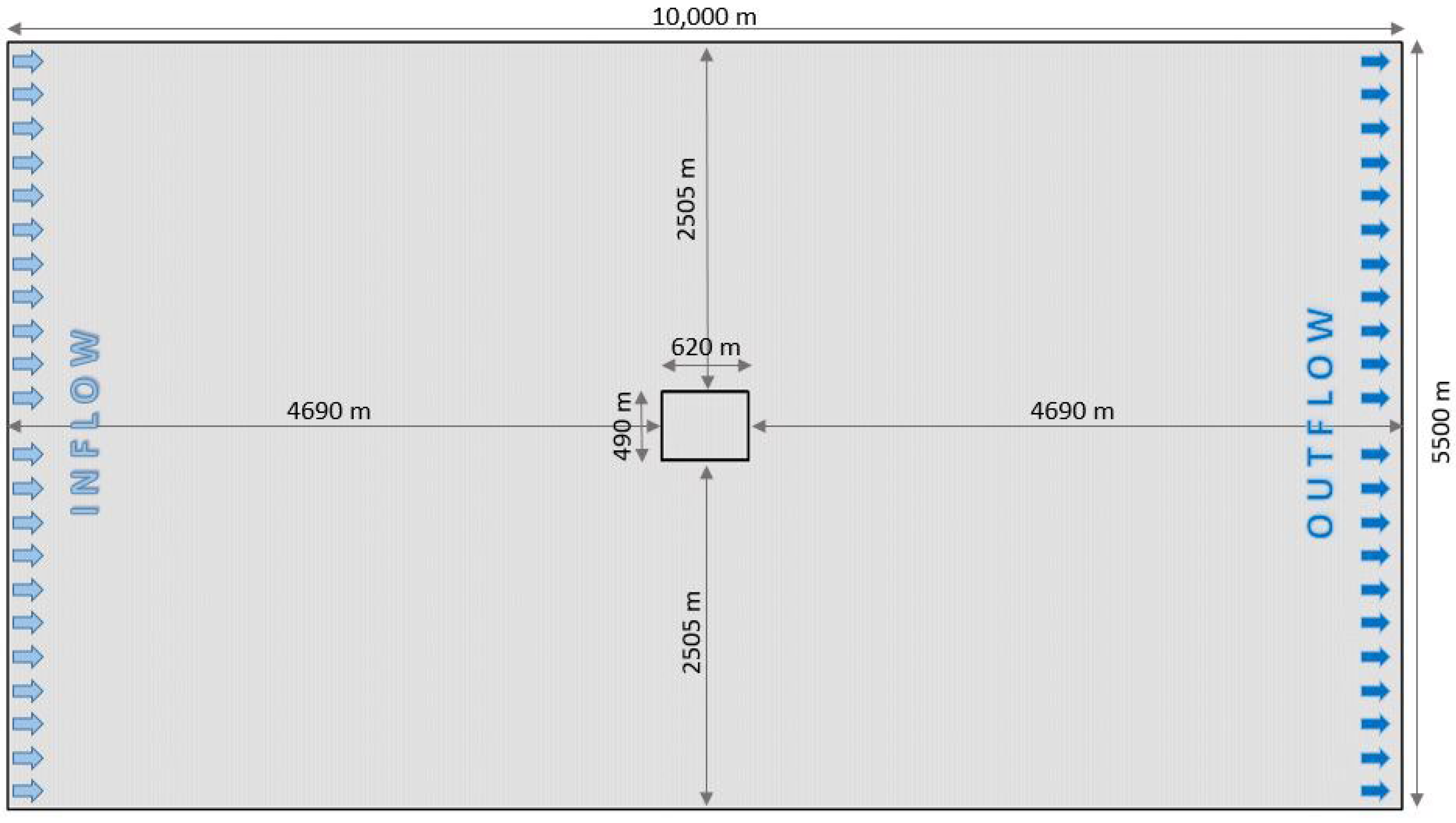
2.2. Conceptual Model

The numerical groundwater flow model is based on a purely theoretical conceptual model with homogenous properties of the saturated zone and geometry presented in Figure 2.

In the rectangular model domain (10,000 m × 5500 m), a pit lake (620 m × 490 m) is located in its center. The long sides of the model domain (10,000 m) and the rectangular pit lake (620 m) are parallel to the groundwater flow direction. Groundwater inflow and outflow are defined by Dirichlet boundary conditions on the left and right sides of the model, respectively. The model is unconfined with hydraulic conductivity (K) of 5 × 10⁻³ ms⁻¹ and effective porosity of 20%. The fully saturated void volume within the pit lake is mimicked by a hydraulic parametrization consisting of high hydraulic conductivity (100 ms⁻¹) and effective porosity of 100% (Figure 3).

Numerical modeling has been performed by FEFLOW (version 7.5) from MIKE Powered by DHI (www.mikepoweredbydhi.com (accessed on 25 May 2023)), which is the one of most widely used software for groundwater flow modeling. FEFLOW solves the groundwater flow equation with the finite-element numerical method [22]. The two-dimensional (2D) model has 2,200,000 quadrilateral elements with a spatial resolution of 5 m × 5 m. In a 2D model, it is assumed that the pit lake extends in the vertical direction from the surface to the bottom of the saturated zone (Figure 3).

Unlike the empirical Equation (1), the slope of the hydraulic head and, therefore, aquifer thickness, can be defined in a numerical model. Several scenarios were considered in this study. They vary in the thickness of the saturated zone and the hydraulic head slope. In order to exclude effects of parameters, which are not considered in Equation (1), for instance, diverse saturated zone thicknesses and slope of the bottom, the hydraulic head and the bottom are parallel in the pre-mining phase in our study. The overview of scenarios is shown in

Table 1. Scenarios for numerical models.

Slope of the Hydraulic Head α	Saturated Zone Thickness
	20 m	80 m
2‰	Scenario 1	Scenario 3
4‰	Scenario 2	Scenario 4

. Furthermore, a three-dimensional (3D) FEFLOW model was developed following the details of Scenario 2 in order to evaluate the potential effects of assumptions that must be made in a 2D model (see Section 4.3).

Each scenario considered two calculations: (a) pre-mining state without the pond in the model (h_PreMS) and (b) post-mining phase with the fully developed pond in the model (h_PostMS). The difference (∆H) of the resulting hydraulic heads is determined for each node of the FEFLOW’s mesh as follows:

$${∆H=h}_{PostMS}-h_{PreMS}$$

(4)

The ∆H is called drawdown when h_PostMS < h_PreMS and mounding when h_PostMS > h_PreMS. For ease of comparison, we selected the 20 cm isoline as the single measure to evaluate the impacts of the scenarios on the hydraulic head.

2.3. Numerical Methods: Governing Groundwater Flow Equation in FEFLOW

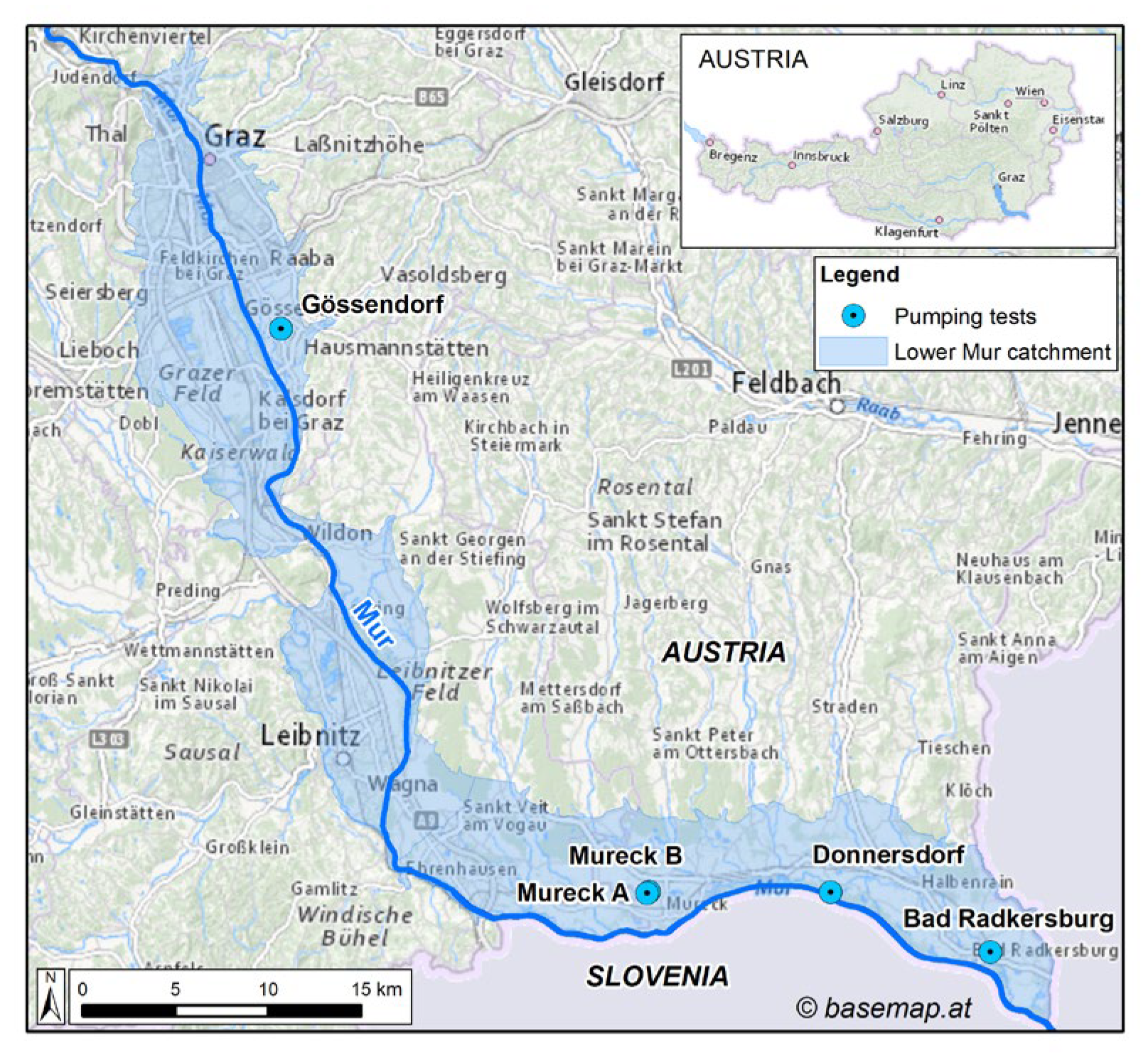
The governing differential equation for 3D unconfined steady-state groundwater flow under anisotropic and heterogeneous conditions can be expressed as follows [15] (p. 77):

$$\frac{\partial }{\partial x}{K}_x\left(h\frac{\partial h}{\partial x}\right)+\frac{\partial }{\partial y}{K}_y\left(h\frac{\partial h}{\partial y}\right)+\frac{\partial }{\partial z}{K}_z\left(h\frac{\partial h}{\partial z}\right)+W=0,$$

(5)

where Kx, Ky, and Kz are the principal components of the hydraulic conductivity tensor K [LT⁻¹], W is a volumetric flux per unit volume and includes sources and/or sinks [LT⁻¹], and $\frac{\partial h}{\partial x}, \frac{\partial h}{\partial y},$ and $\frac{\partial h}{\partial z}$ are the components of the vector grad h—the gradient of hydraulic head (h) [L], which implies the Darcy‘s law as follows:

$$q=-K\times grad h=-K\times \sin \alpha ,$$

(6)

where q is a specific flux [LT⁻¹] and α slope of the phreatic surface [−] [15] (p. 77), [23] (p. 361).

The saturated zone in an unconfined porous medium with a phreatic surface forms a layer with a time-depended thickness B(x₁, x₂, t). In this case, the bottom f^B (x₁, x₂) is considered stationary, while the surface of the layer (which is equal to the hydraulic head in an unconfined porous medium, h(x₁, x₂, t) can change in time [22] (p. 131):

$$B\left(x_1,x_2,t\right)=h\left(x_1,x_2,t\right)-f^B\left(x_1,x_2\right).$$

(7)

In order to reduce the 3D groundwater flow equation to a 2D essentially horizontal equation in an unconfined porous medium, where the gravity effects are ignored, the horizontal extent of a regional flow field must be much bigger than the thickness of the saturated zone [22] (p. 64). Such a relationship guarantees a small slope of the phreatic surface (α), which is needed for the Dupuit–Forchheimer simplification of the specific Darcy flux (Equation (6)). In addition to the dominantly horizontal flow, the Dupuit–Forchheimer simplification assumes a homogeneous and isotropic porous medium. Nevertheless, the vertical flow is not ignored even though vertical hydraulic head gradients are assumed to be negligible [15] (pp. 120–124).

Various variants of the 2D groundwater flow equation (e.g., Boussinesq equation, Laplace equation) have been later derived under the Dupuit–Forchheimer assumptions [23] (pp. 377–378). Nevertheless, Equation (8) is the basic vertically averaged (2D) equation for a steady-state groundwater flow in an unconfined porous medium under Dupuit–Forchheimer simplifications implemented in FEFLOW [22] (p. 407).

$$\overline{\mathit{Q}}=\mathbf{\nabla }\times \overline{\mathit{q}},$$

(8)

$$\overline{\mathit{q}}=-\mathit{B}\mathit{K}\times \mathbf{\nabla }\mathit{h},$$

(9)

where h is hydraulic head [L],$\overline{\mathit{q}}=\mathit{B}\times \mathit{q}$ is depth-integrated Darcy velocity [LT⁻¹], B is a thickness [L] of a saturated zone (h − f^B), $\overline{\mathit{Q}}$ is the depth-integrated source/sink term [−], K is tensor of hydraulic conductivity [L²T⁻¹], and f^B is the bottom bounding surface [L].

2.4. Pumping Test

Five pumping tests have been performed in the quaternary aquifer of the Lower Mur catchment in Austria. The selected wells named Gössendorf, Mureck A, Mureck B, Donnersdorf, and Bad Radkersburg are shown in Figure 4. Details of the data analysis and interpretation are discussed elsewhere [24,25].

The purpose of the pumping tests in this study is to compare the radius of influence (R_ZOI) observed during pumping tests to the R_ZOI computed by Equation (3).

3. Results

3.1. Empirical Method after Wrobel

Equation (1) was solved for two scenarios that differ in slopes of the hydraulic head. The results are presented in

Table 2. Scenarios for numerical model runs.

Slope of the Hydraulic Head [‰]	Vertical Drawdown s [m]	Horizontal Drawdown R [m]
2	0.6	171.2
4	1.2	342.4

. The calculations considered the following parameters: B = 490 m, K = 5 × 10⁻³ ms⁻¹ and length of the pit lake of 620 m. Parameter R in Wrobel’s equation returns drawdown extensions in only one direction, which is parallel to the given regional groundwater flow and is measured upstream from the left pit lake’s edge.

In order to make empirical and numerical results comparable the vertical drawdown s is calculated from the hydraulic head slope (α) and the pit lake’s length (620 m). As expected, due to the linear relationship between parameters R and s in Equation (1), the horizontal drawdown increases by a factor of two if the slope of the hydraulic head is doubled.

3.2. Numerical Simulations

Figure 5 shows the 20 cm isolines of drawdown and mounding (explained in Section 2.2) that result from the four scenarios listed in Table 1. The shape of the drawdown area expands widely transversal to the direction of groundwater flow, when the hydraulic head slope is 4‰, while it expands quite evenly in all directions (~950 m) as the hydraulic head gradient is only 2‰. The mounding area is smaller than the drawdown area for all four scenarios. When the slope of the hydraulic head slope is 4‰, the mounding shape is more circular compared to an ellipsoid shape of the drawdown area upstream of the pit lake. Moreover, the larger saturated zone thickness leads to a greater extent of the mounding area for the same hydraulic head slope, which is the opposite for the drawdown area. For the scenario with increased hydraulic head slope, the drawdown isolines show a clear anisotropic behavior which is more pronounced in the case of the smaller saturated zone thickness. Overall, the hydraulic head slope shows a more pronounced impact on the hydraulic head distortion by the pit lake than the saturated zone thickness. Increasing saturated zone thickness leads to a greater extent of the mounding area in the flow direction, but to a lesser extent transversal to the flow direction in the drawdown area.

Empirical results presented in Section 3.1 were compared with numerically computed extensions of the drawdown. In general, numerical results are approximately six-times larger than empirical results, deviations between them increase with the increasing hydraulic head slope. For instance, drawdown extensions in scenarios with α = 4‰ are ~2050 m (numerical result) and only 342 m (empirical result). In scenarios with α = 2‰ extensions of the drawdown are ~950 m (numerical result) and 171 m (empirical result).

Figure 6 shows the differences of the hydraulic heads in all four scenarios (∆H calculated by Equation (4)), following a longitudinal profile from the inflow to the outflow boundaries. The maximal drawdown and mounding are clearly on the edges of the pond. The lowest hydraulic head is approximately 0.6 m or 1.4 m below the initial hydraulic head for the hydraulic head gradients 2‰ and 4‰, respectively. The ∆H in the mounding area is slightly smaller, i.e., the hydraulic head is 0.6 m or 1.2 m above the initial hydraulic head for the hydraulic head gradients of 2‰ and 4‰, respectively.

4. Discussion

4.1. Comparison of Groundwater Drawdowns Calculated with Empirical and Numerical Methods

To evaluate the results of the drawdown due to a pit lake by applying the empirical equation after Wrobel (1980) [19], a 2D groundwater flow model was built in FEFLOW. The numerical model approximates as closely as possible the conditions on which Equation (1) was derived such as homogeneous hydraulic conductivity value, steady-state conditions, and longer face of the rectangular gravel pit lake being perpendicular to the groundwater flow direction. In addition, the model has a parallel bottom and surface with a slight inclination. Results as described in Section 3.2, of such a simple numerical model significantly differ from those calculated by Equation (1). In fact, the difference between the hydraulic heads at the pre-mining and the post-mining stages (i.e., ∆H in Equation (4)) is significantly underestimated by Equation (1) in comparison to FEFLOW results (see Section 3.2).

It was observed that the hydraulic head changes (i.e., ∆H in Equation (4)) are more sensible on the gradient of the hydraulic head than on the thicknesses of the saturated zone. Figure 5 shows a smaller horizontal extension of the drawdown area and a larger horizontal extension of the mounding area when the saturated zone is thicker, and a larger ∆H when the hydraulic head is steeper. The ∆H at the edge of the pit lake is up to approximately 0.8 m larger when the hydraulic head slope is 4‰ in comparison to the hydraulic head slope of 2‰ (Figure 6).

Although a laminar flow is assumed in the 2D model, Wang et al. (2013) [26] demonstrated that the Dupuit–Forchheimer assumptions give a good approximation of hydraulic head for an unconfined aquifer, whose gradient is less than 5.7° (100‰). Therefore, it can be concluded that the error associated to the sloping base of the saturated zone in our study is negligible. Furthermore, Equation (1) considers very roughly the saturated thickness and the hydraulic head gradient via the scaling parameter. Such a simplification can obviously lead to inaccurate and potentially misleading results. Nevertheless, the numerical method has a great advantage over the empirical method in respect to the ability of incorporating spatially distributed dataset into the analysis.

In order to see an effect of one of the spatially distributed datasets on the drawdown and mounding areas, additional scenarios with a horizontal bottom slope, which often appears in the real world, were calculated. Due to the horizontal bottom (0 m), these scenarios differ from those in Table 1 in the uneven thickness of the saturated zone, which decreases from the inflow- to the outflow-borders of the model domain. The results show larger mounding area in comparison to the drawdown area. Their difference increases with the larger initial slope of the hydraulic head. Also, drawdown area is smaller and mounding area is larger in comparison to the results where the bottom slope is equal to the hydraulic head slope. This leads to a slightly smaller discrepancy of the drawdown area for scenarios with the horizontal bottom from the drawdown area computed by Equation (1).

The tilting line denotes the line at which the lake water level in the post-mining phase and the groundwater level in the pre-mining phase have the same elevation. According to Lübbe (1977) [11], the tilting line should be located in the center of a pit lake (perpendicular to the water flow direction). In the longitudinal cross section in Figure 7, the hydraulic heads for the pre- and post-mining phases do not exactly follow Lübbe’s concept [11]. Instead, the tilting line derived by the FEFLOW’s computations is shifted about 45 m from the center of the pit lake in the direction of the model’s outflow border in Scenario 2. The reason is that the 2D flow Equation (5) in FEFLOW under the Dupuit–Forchheimer assumptions is non-linear, and it follows a second-order derivative. The Dupuit–Forchheimer assumptions are described in Section 2.3. Shifted tilting lines with a parabolic surface of the hydraulic head are also shown in Jost et al. (2023) [27].

In addition to the thickness of the saturated zone and the hydraulic head slope, the extensions of drawdown and mounding areas also depend on the local hydraulic conductivity distribution, the shape of the pit lake, its depth and hydraulic connection to any other surface water bodies [7,27,28]. Although the evaluation of each potential effect of a gravel pit lake on groundwater is not the subject of this paper, they can be accurately implemented in a numerical model. Jost et al. (2023) [27] studied the influences of geometrical, hydrodynamical and meteorological factors on the groundwater level and water balances. The potential errors by ignoring these parameters have to be considered during the result analysis of an individual project.

A numerical model requires additional information for its parametrization, which may be considered impractical due to the frequent lack of required data, high costs, and time-consuming work. Therefore, it is considered a useful tool only in the advanced stages of gravel mining, when more hydrogeological datasets are available for a study area [12,13,18]. Nevertheless, our study shows that in the context of pit lakes, even extremely simple 2D numerical models can provide more accurate results than the empirical approach. Therefore, we propose to use simple numerical models already in the initial stages of gravel mining to properly evaluate potential environmental impacts associated with the pit lake. As soon as new data is available, such models can be calibrated (or re-calibrated) on demand.

4.2. Radius of Influence Calculated by Sichardt’s Equation Compared to Field Data from Pumping Tests

As described in Section 2.1, Wrobel’s equation (Equation (1)) is based on Sichardt’s equation (Equation (3)). The latter is used to calculate the extent to which the hydraulic head is influenced by pumping from a vertical well (the radius of influence R_ZOI). However, larger radii of influence in pumping tests than those calculated by Equation (3) have been reported by Yihdego (2018) [18] and Fuleccia (2015) [12]. Desens and Houben (2022) [29] proposed correction factors for Equation (3), which are intended for case studies with different porosities and saturated zone thicknesses.

For the reasons mentioned above, five pumping tests, as shown in Figure 4, were performed in the quaternary aquifer of the Lower Mur catchment in Austria. The saturated thicknesses measured at the five wells range between 4 m and 13 m, the observed vertical drawdowns vary from 0.8 m to 1.4 m and the resulting hydraulic conductivities fluctuate between 2 × 10⁻³ ms⁻¹ and 9 × 10⁻³ ms⁻¹. Thus, the hydrogeological conditions observed at these five wells are similar to the ones considered in the derivation of the empirical Equation (1).

The radii of influence (R_ZOI) at the five wells caused by the groundwater withdrawal have been delineated from groundwater level readings obtained at the observation wells. It turned out that these R_ZOI were between 1.25 and 6 times larger than the values calculated by Equation (3). In order to fit R_ZOI calculated by Equation (3) with field data from the five pumping tests, an individual scaling factor for Equation (3) was adjusted accordingly to each pumping well. The new scaling factors fluctuate between 3750 and 18,000, which clearly deviates from its original value of 3000.

The extensions of the horizontal drawdown calculated by Equation (1) are also smaller compared to the numerical results driven by FEFLOW (Figure 5). The drawdown of 20 cm is approximately up to six times more distant from the pit lake in the 2D model compared to Equation (1). Additionally, it has to be considered that in the evaluation of the groundwater flow model results the drawdown isoline at 20 cm was investigated. This means that the actual drawdown area extends even wider. Hence, it can be assumed that the empirical Equations (1) and (3) fundamentally underestimate the extension of the drawdown area related to a pit lake or groundwater pumping.

These results underline our hypothesis that a unique scaling factor in Equation (1) cannot adequately account for the various subsurface characteristics, which are relevant for calculating the drawdown area. For example, the length of the pit lake and the slope of the hydraulic head are only superficially integrated in Equation (1) through the parameter s (see Section 2.1), although they can affect the range of drawdown. Furthermore, the shape of the pit lake, its position with respect to the groundwater flow direction and thickness of the saturated zone, which affect the drawdown as well, cannot be incorporated in Equation (1). All these facts make Equation (1) inadequate for calculating the drawdown area caused by a specific pit lake in complex hydrogeological conditions.

4.3. 2D vs. 3D Numerical Model in FEFLOW

Groundwater flow is in principle a three-dimensional (3D) problem, thus a simplified 2D model under Dupuit–Forchheimer assumptions has certain limitations (see Section 2.3). Nevertheless, the 2D model often provides sufficient results, especially when it comes to large regional models. A 2D model requires significantly less time and costs for its implementation. Also, shorter running times give better chances to have a good calibration and facilitate uncertainty analysis [15] (p. 122). The use of a 2D model can be often questionable, especially when the saturated zone has a non-horizontal surface and bottom and heterogeneous distributions of hydrogeological parameters. For instance, Bresciani et al. (2014) [30] have questioned whether the Dupuit–Forchheimer assumption can be suitable for predicting the groundwater seepage area in hillslopes.

A further analysis was carried out with a 3D numerical model to evaluate the simplifications considered in the 2D model. This analysis is based only on Scenario 2 (see Table 1) and the computed areas of drawdown and mounding between the two models have been compared as shown in Figure 8. In contrast to the 2D model, a 3D model does not neglect the vertical hydraulic gradient, thus it can offer full flexibility regarding the heterogeneity of the study domain and implementation of a pit lake’s depth. This is particularly important when the bottom of the pit lake does not coincide with the aquifer bottom.

For the comparison, a four-layer 3D model was built in FEFLOW. Here, the pit lake in the post-mining phase is extended from the surface to the bottom of the saturated zone analogue to the 2D model. The horizontal discretization in all the layers is the same as in the 2D FEFLOW model, i.e., quadrilateral elements of 5 m.

Figure 8 shows small deviations between the sizes of the drawdown and mounding areas at 20 cm in the 2D and 3D models. On one hand, the extension of the drawdown area is up to 180 m in the direction of groundwater flow and 300 m perpendicular to the groundwater flow direction larger in the 2D model than in the 3D model. The shapes of the drawdown isolines follow an elliptical form in both modeling cases. On the other hand, the extension of the mounding areas is similar for both models and exhibits a circular form. In comparison to the 2D model, the 3D modeling approach slightly reduces the underestimation of the drawdown area calculated by the empirical Wrobel’s equation (see yellow line in Figure 8). The extensions of drawdown areas in the 2D and 3D models deviate for about 210 m.

The tilting line in the 3D model is also not located in the center of the pit lake, which indicates the non-linearity of the 3D model.

5. Conclusions

The assignment of the mining rights in pit lakes often depends on the extension of hydraulic head changes. These estimations are typically based on simplified empirical equations. However, such an empirical approach cannot account for real hydrogeological complexities and thus can lead to underestimation of the affected areas [12]. An underestimation of the drawdown zones may deteriorate groundwater conditions, for instance through contamination and groundwater warming [31]. For this reason, this paper compared groundwater drawdowns caused by an open gravel pit lake that is derived by the empirical Wrobel’s equation and numerical methods. Results show significantly underestimated drawdown area, which is calculated by the empirical Wrobel’s equation compared to the results obtained from a two-dimensional (2D) groundwater flow model. Numerical computations demonstrate that the slope has a larger effect on the extent of the drawdown and mounding areas as the thickness of the saturated zone. Additionally, the potential error of using 2D model for solving a three-dimensional (3D) groundwater flow problem was evaluated with a 3D FEFLOW model. The modeling exercises showed that the 2D numerical approach leads to larger drawdown areas, whereas the mounding area was marginally wider in the 3D model.

Based on this study can be said that Wrobel’s equation is not appropriate for calculating drawdowns caused by pit lakes under heterogeneous conditions. Wrobel’s equation considers the slope only indirectly by calculating the drawdown and it does not include the thickness of the saturated zone. It has been even shown that Sichardt’s equation, from which Wrobel’s equation has been derived, provides misleading results too. Thus, it is worth investing in numerical models for the purpose of risk assessment, because they do provide more comprehensive and spatially distributed results. In fact, they can be used as a base for selecting more effective measures for groundwater protection. Many study sites meet requirements for using a much less demanding 2D model instead of a complicated 3D model. The 3D model provides more precise results than the 2D model, while the 2D model, despite its simplifications, often proves to be a good compromise, especially when it comes to regional models.

The findings of this paper have to be investigated further, e.g., to evaluate the impact of transient conditions or subsurface heterogeneity. Nevertheless, we recommend the stakeholders avoid using empirical equations for risk assessment analysis of pit lakes.

References

1. Eynard, U.; Georgitzikis, K.; Wittmer, D.; El Latunussa, C.; Torres de Matos, C.; Mancini, L.; Unguru, M.; Blagoeva, D.; Bobba, D.; Pavel, C.; et al. Study on the EU’s List of Critical Raw Materials (2020): Non-Critical Raw Materials Factsheets (Final); European Commission: Brussels, Belgium, 2020. [Google Scholar] [CrossRef]
2. Highley, D.; Harrison, D.; Cameron, D.; Lusty, P.; Cowley, J.; Rayner, D. Mineral Planning Factsheets: Construction Aggregates; Brown, T., Ed.; BGS: London, UK, 2019. [Google Scholar]
3. EEA (European Environmental Agency). Effectiveness of Environmental Taxes and Charges for Managing Sand, Gravel and Rock Extraction in Selected EU Countries; EEA Report, No. 2/2008; EEA: Copenhagen, Denmark, 2008. [Google Scholar] [CrossRef]
4. UEPG (European Aggregates Association). Annual Review 2020–2021. Available online: https://www.aggregates-europe.eu/wp-content/uploads/2023/03/Final_-_UEPG-AR2020_2021-V05_spreads72dpiLowQReduced.pdf (accessed on 3 May 2023).
5. Schultze, M.; Vandenberg, J.; McCullough, C.D.; Castendyk, D. The Future Direction of Pit Lakes: Part 1, Research Needs. Mine Water Environ. 2022, 41, 533–543. [Google Scholar] [CrossRef]
6. Kidmose, J.; Engesgaard, P.; Nilsson, B.; Laier, T.; Looms, M.C. Spatial Distribution of Seepage at a Flow-Through Lake: Lake Hampen, Western Denmark. Vadose Zone J. 2011, 10, 110–124. [Google Scholar] [CrossRef]
7. Mollema, P.; Antonellini, M. Water and (Bio)Chemical Cycling in Gravel Pit Lakes: A Review and Outlook. Earth Sci. Rev. 2016, 159, 247–270. [Google Scholar] [CrossRef]
8. Muellegger, C.; Weilhartner, A.; Battin, T.J.; Hofmann, T. Positive and Negative Impacts of Five Austrian Gravel Pit Lakes on Groundwater Quality. Sci. Total Environ. 2013, 443, 14–23. [Google Scholar] [CrossRef]
9. Castendyk, D.N.; Eary, L.E.; Balistrieri, L.S. Modeling and Management of Pit Lake Water Chemistry 1: Theory. Appl. Geochem. 2015, 57, 267–288. [Google Scholar] [CrossRef]
10. Søndergaard, M.; Lauridsen, T.L.; Johansson, L.S.; Jeppesen, E. Gravel Pit Lakes in Denmark: Chemical and Biological State. Sci. Total Environ. 2018, 612, 9–17. [Google Scholar] [CrossRef] [PubMed]
11. Lübbe, E. Schriftenreiche des Kuratoriums für Wasser und Kulturbauwesen, Heft 29, Baggerseen, Bestandsaufnahme, Hydrologie und planerische Konsequenzen; Paul Parey: Hamburg/Berlin, Germany, 1977; ISBN 3-490-02997-6. [Google Scholar]
12. Fileccia, A. Some Simple Procedures for the Calculation of the Influence Radius and Well Head Protection Areas (Theoretical Approach and a Field Case for a Water Table Aquifer in an Alluvial Plain). AS/IT JGW 2015, 4, 7–23. [Google Scholar] [CrossRef]
13. Arnold, L.R.; Langer, W.H.; Paschke, S.S. Analytical and Numerical Simulation of the Steady-State Hydrologic Effects of Mining Aggregate in Hypothetical Sand-and-Gravel and Fractured Crystalline-Rock Aquifers; Water-Resource Investigations Report 02-4267; USGS: Denver, CO, USA, 2003. Available online: https://pubs.usgs.gov/wri/2002/4267/report.pdf (accessed on 23 May 2023).
14. Brownlee, J. Machine Learning Mastery. Analytical vs Numerical Solutions in Machine Learning. Available online: https://machinelearningmastery.com/analytical-vs-numerical-solutions-in-machine-learning/ (accessed on 26 April 2023).
15. Anderson, M.P.; Woessner, W.W.; Hunt, R.J. Applied Groundwater Modelling: Simulation of Flow and Advective Transport, 2nd ed.; Elsevier Inc.: Sand Diego, CA, USA, 2015. [Google Scholar] [CrossRef]
16. Marinelli, F.; Niccoli, W.L. Simple Analytical Equations for Estimating Ground Water Inflow to a Mine Pit. Ground Water 2000, 38, 311–314. [Google Scholar] [CrossRef]
17. Kandelous, M.K.; Šimůnek, J. Comparison of Numerical, Analytical, and Empirical Models to Estimate Wetting Patterns for Surface and Subsurface Drip Irrigation. Irrig. Sci. 2010, 28, 435–444. [Google Scholar] [CrossRef]
18. Yihdego, Y. Engineering and Enviro-Management Value of Radius of Influence Estimate from Mining Excavation. J. Appl. Water Eng. Res. 2018, 6, 329–337. [Google Scholar] [CrossRef]
19. Wrobel, J.P. Wechselbeziehungen zwischen Baggerseen und Grundwasser in gut durchlässigen Schottern. GWF Wasser/Abwasser 1980, 121, 165–173. [Google Scholar]
20. Niemeyer, R. Hydrologische Untersuchungen an Baggerseen und Alternativen der Folgenutzung; Lehrstuhl für Landwirtschaftl. Wasserbau u. Kulturtechnik, Inst. für Städtebau, Bodenordnung u. Kulturtechnik d. Univ.: Bonn, Germany, 1978. [Google Scholar]
21. Kyrieleis, W.; Sichardt, W. Grundwasserabsenkung bei Fundierungsarbeiten; Julius Springer: Berlin, Germany, 1930. (In German) [Google Scholar]
22. Diersch, H.-J.G. FEFLOW—Finite Element Modeling of Flow, Mass and Heat Transport in Porous and Fractured Media; Springer: Berlin/Heidelberg, Germany, 2014. [Google Scholar] [CrossRef]
23. Bear, J. Dynamics of Fluids in Porous Media; Dover Publications, Inc.: New York, NY, USA, 1972. [Google Scholar]
24. Fank, J.; Wieser, L. Mureck VFB2 Neuerrichtung, Hydrogeologisches Gutachten; JR-AquaConsol GmbH: Graz, Austria, 2021. (In German) [Google Scholar]
25. Fank, J.; Mach, J. SI-MUR-AT, Optimierung Brunnenfeld Mureck des Wasserverbandes “Wasserversorgung Grenzland Südost”; Grundwasserhydrologisches Gutachten; JR-AquaConsol GmbH: Graz, Austria, 2018. (In German) [Google Scholar]
26. Wang, Q.; Zhan, H.; Tang, Z. A New Package in MODFLOW to Simulate Unconfined Groundwater Flow in Sloping Aquifers. Groundwater 2014, 52, 924–935. [Google Scholar] [CrossRef] [PubMed]
27. Jost, A.; Wang, S.; Verbeke, T.; Colleoni, F.; Flipo, N. Hydrodynamic Relationships Between Gravel Pit Lakes and Aquifers: Brief Review and Insights from Numerical Investigations. CR GEOSCI 2023, 355, 1–25. [Google Scholar] [CrossRef]
28. Hofman, T.; Müllegger, C. Einfluss von Nassbaggerungen auf die Oberflächen- und Grundwasserqualität; Abschlussbericht; Vienna University: Vienna, Austria, 2011. (In German) [Google Scholar]
29. Desens, A.; Houben, G.J. Jenseits von Sichardt—Empirische Formeln zur Bestimmung der Absenkreichweite eines Brunnens und ein Verbesserungsvorschlag. Grundwasser 2022, 27, 131–141. [Google Scholar] [CrossRef]
30. Bresciani, E.; Davy, P.; de Dreuzy, J.R. Is the Dupuit assumption suitable for predicting the groundwater seepage area in hillslopes? Water Resour. Res. 2014, 50, 2394–2406. [Google Scholar] [CrossRef]
31. Ahern, J.A. Ground-Water Capture-Zone Delineation: Method Comparison in Synthetic Case Studies and a Field Example on Front Wainwright, Alaska. Master’s Thesis, University of Alaska Fairbanks, Fairbanks, Alaska, 2005. Available online: https://scholarworks.alaska.edu/handle/11122/6942 (accessed on 23 May 2023).
Figure 1. Graphical presentation of parameters in the Wrobel’s equation (adopted after [20]).
Hydrology 10 00140 g001
Figure 2. Geometry of the conceptual model.
Hydrology 10 00140 g002
Figure 3. Longitudinal model profile.
Hydrology 10 00140 g003
Figure 4. Locations of wells in the Lower Mur catchment in Austria, where pumping tests have been performed.
Hydrology 10 00140 g004
Figure 5. Drawdown calculated by Wrobel’s equation, drawdown/mounding at 20 cm for Scenarios 1–4 (Table 1).
Hydrology 10 00140 g005
Figure 6. Drawdown and mounding in a vertical cross section for Scenarios 1–4 (Table 1), computed with FEFLOW (∆h thickness of the saturated zone, α-slope of the hydraulic head).
Hydrology 10 00140 g006
Figure 7. Hydraulic heads in the longitudinal cross section in pre- and post-mining phases for Scenario 2 (∆h thickness of the saturated zone, α-slope of the hydraulic head).
Hydrology 10 00140 g007
Figure 8. Hydraulic head changes for Scenario 2 in the 2D and four-layer 3D groundwater models.
Hydrology 10 00140 g008