

Simulating Groundwater Potential Zones in Mountainous Indian Himalayas—A Case Study of Himachal Pradesh


 ,
,  ,
,  ,
,  , ,
, ,
Abstract
:1. Introduction
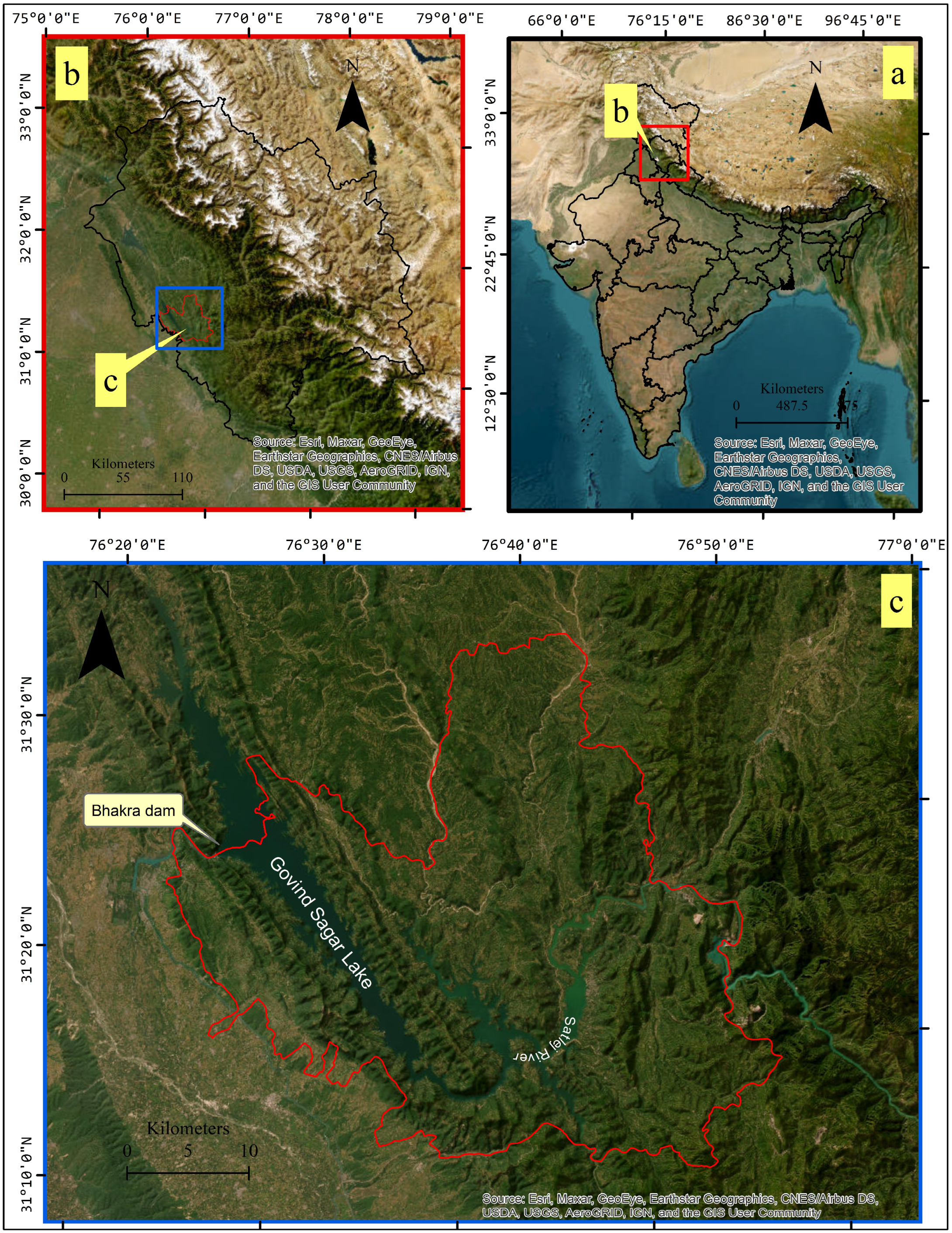
2. Study Area
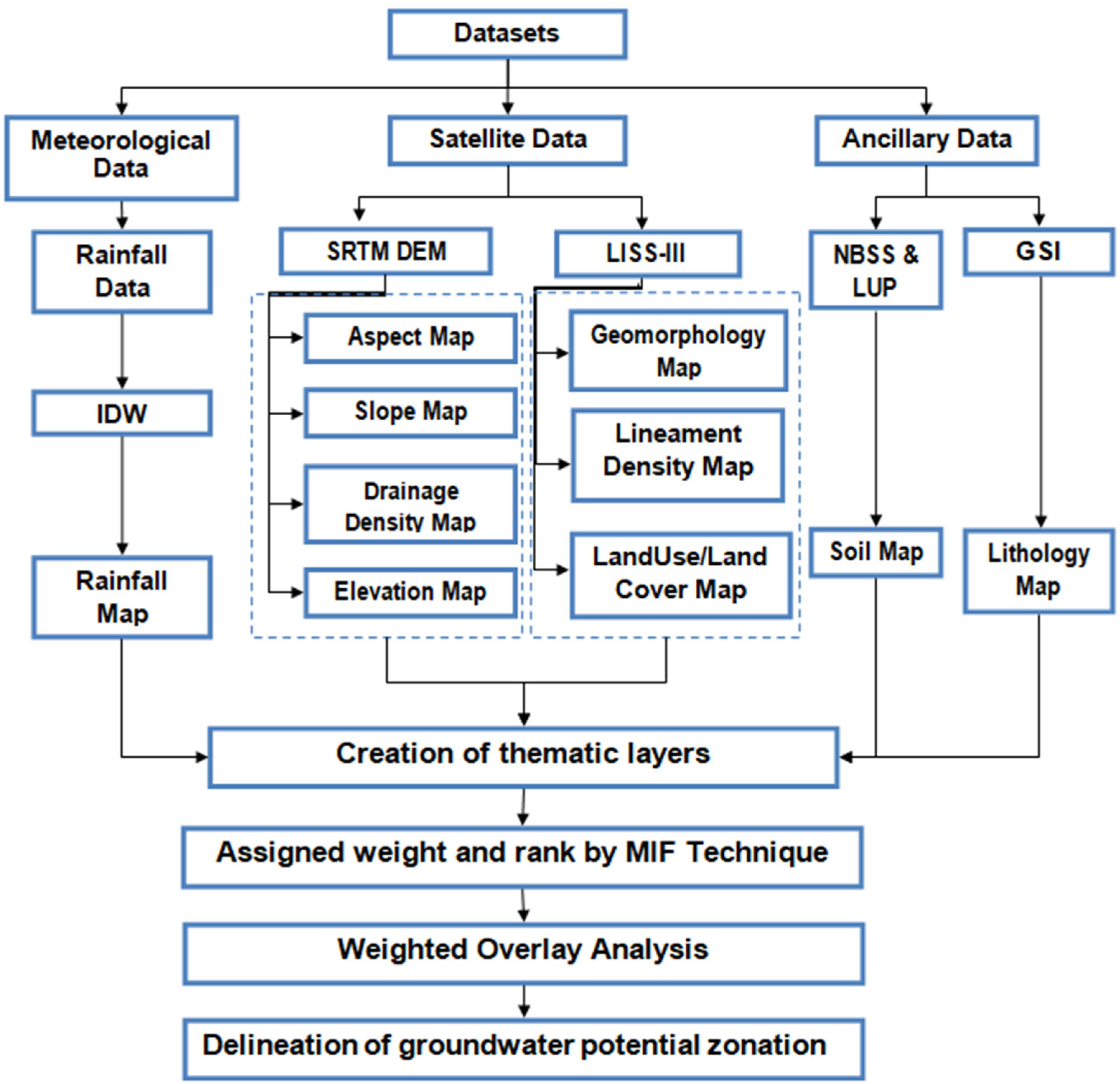
3. Materials and Methods
3.1. Dataset Used and Preparation of Thematic Maps
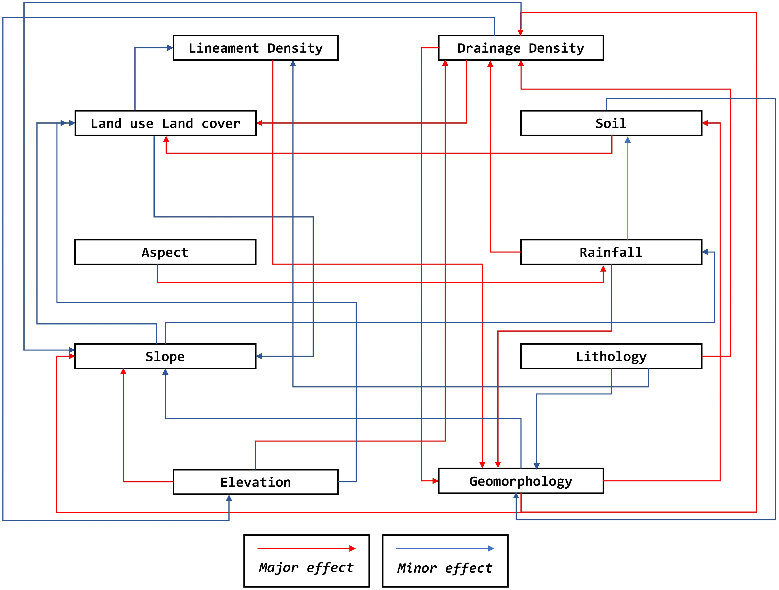
3.2. Calculation of Weightage of MI Factors for Zonation of Groundwater Potential
4. Results and Discussion
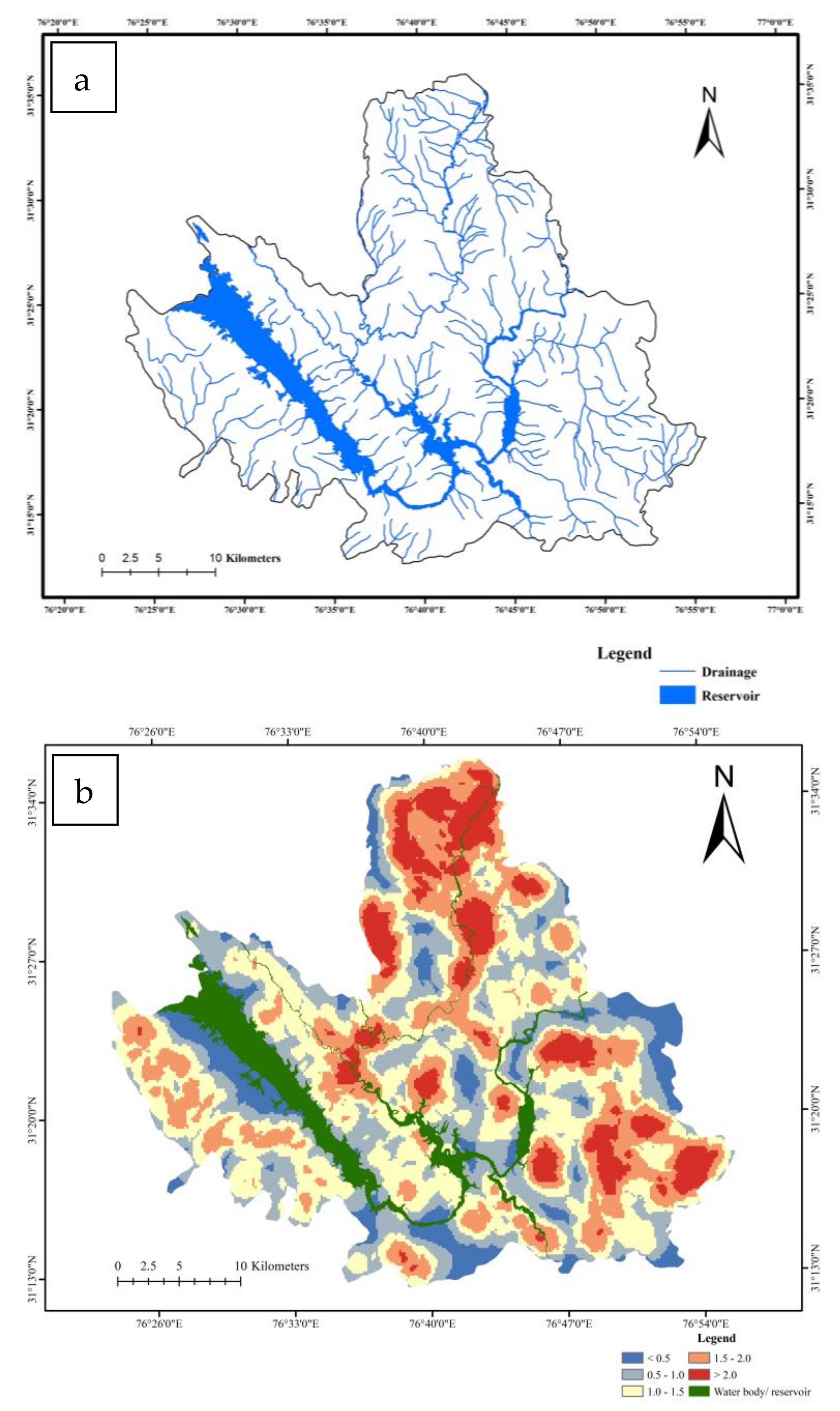
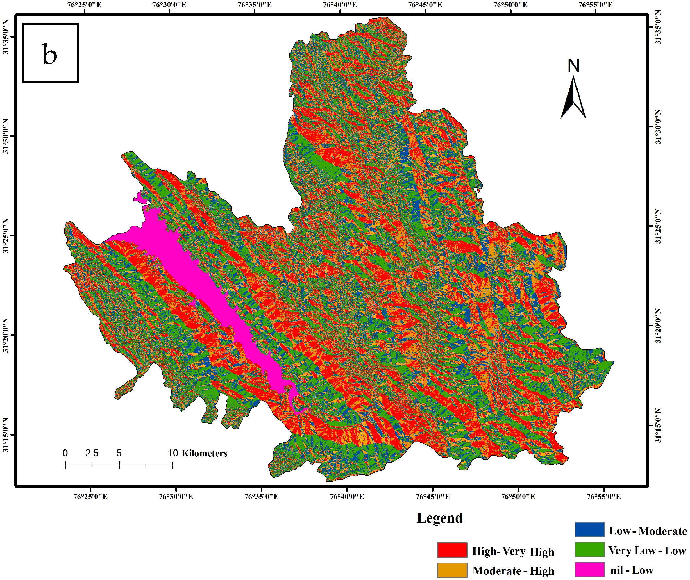
4.1. Analysing Drainage Density
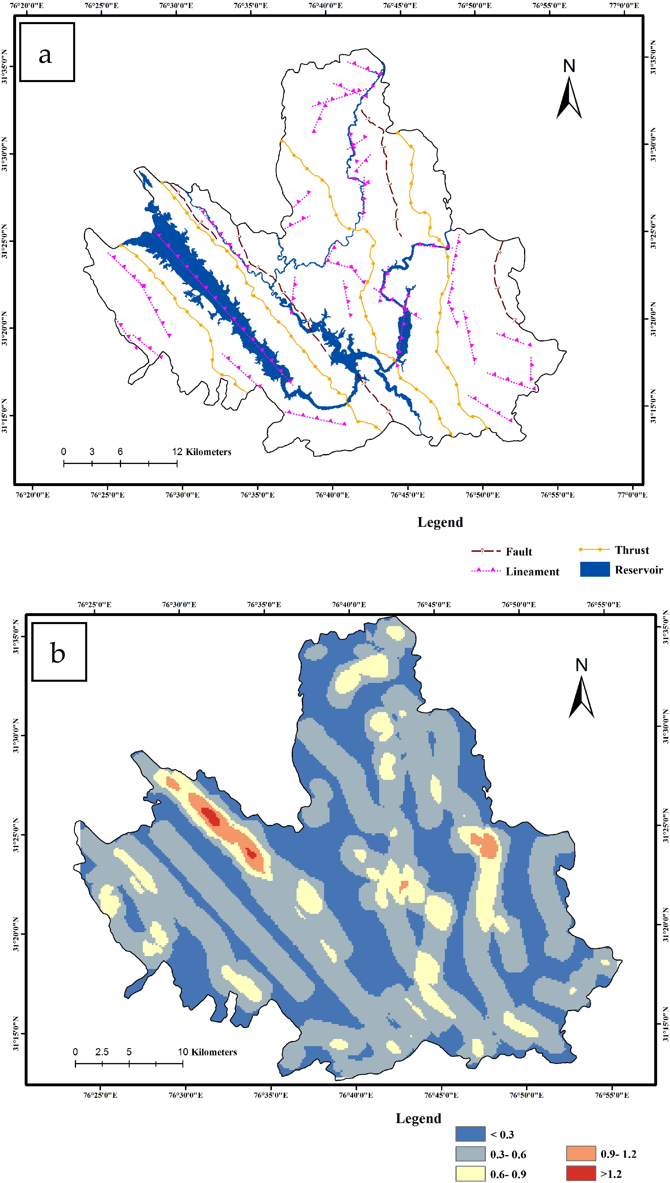
4.2. Lineament Density Analysis
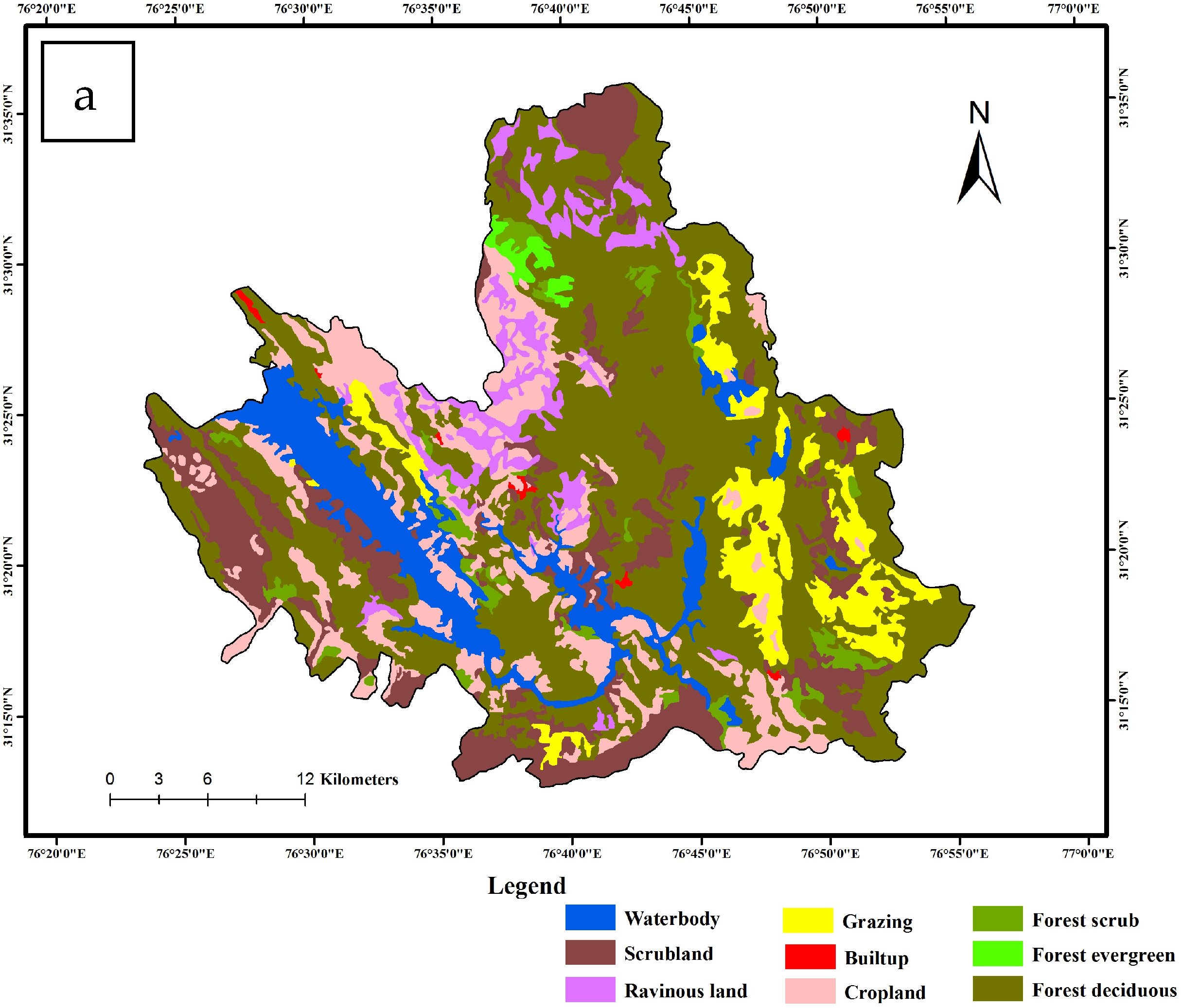
4.3. Land Use and Land Cover Analysis
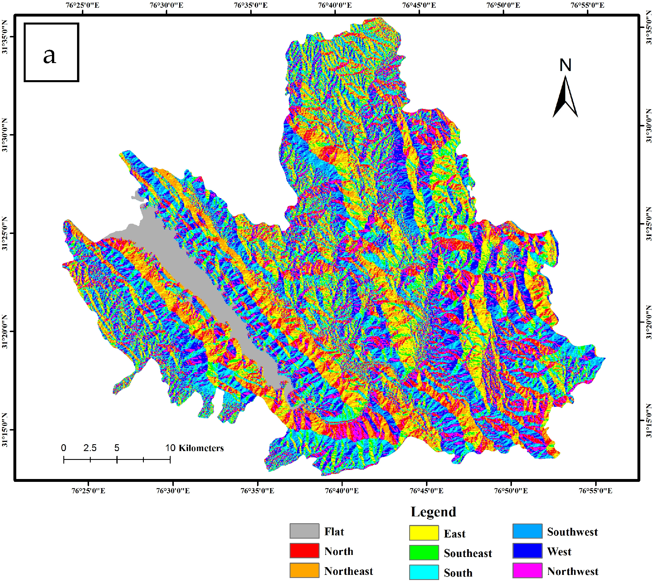
4.4. Aspect Analysis
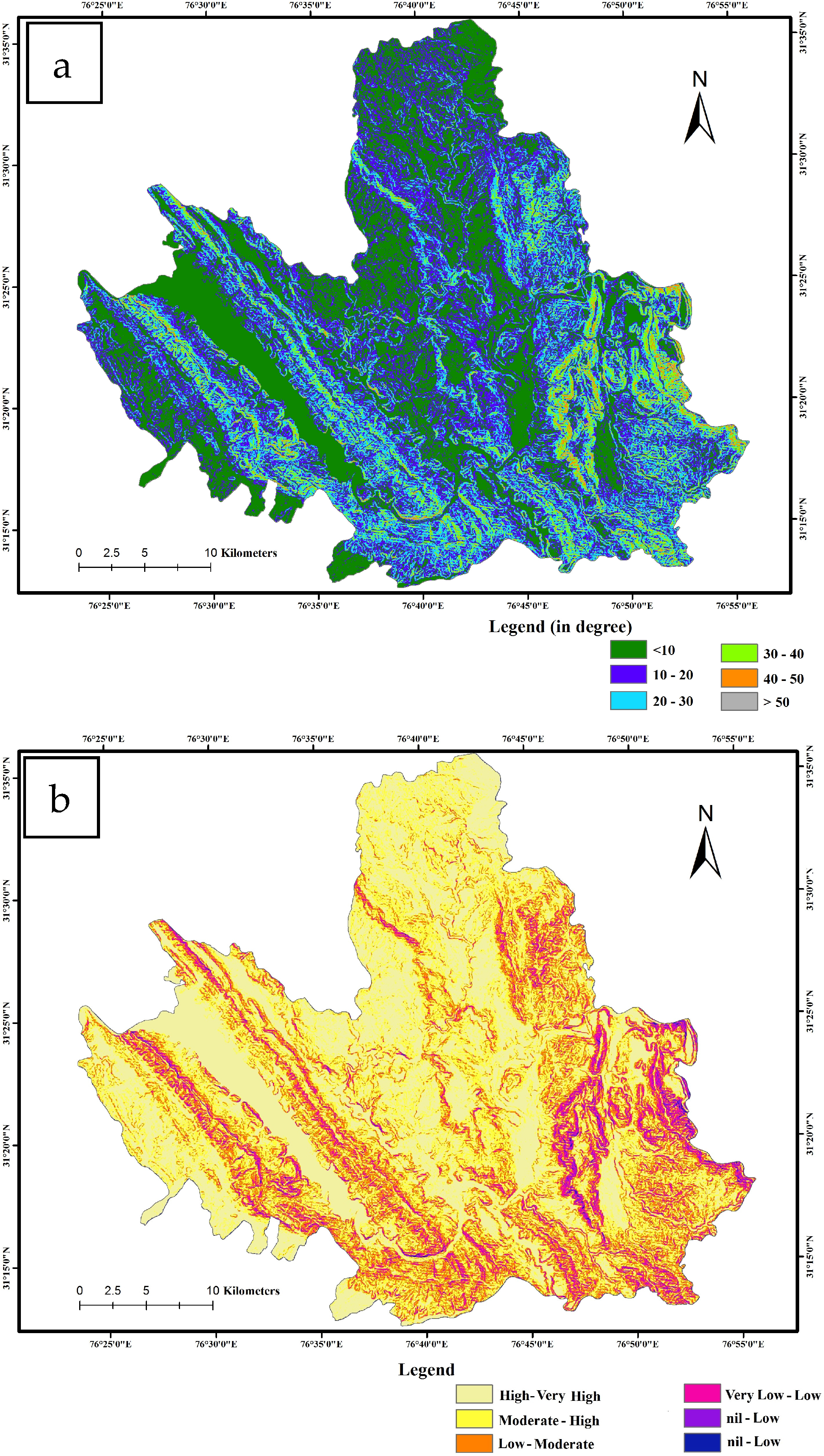
4.5. Slope Analysis
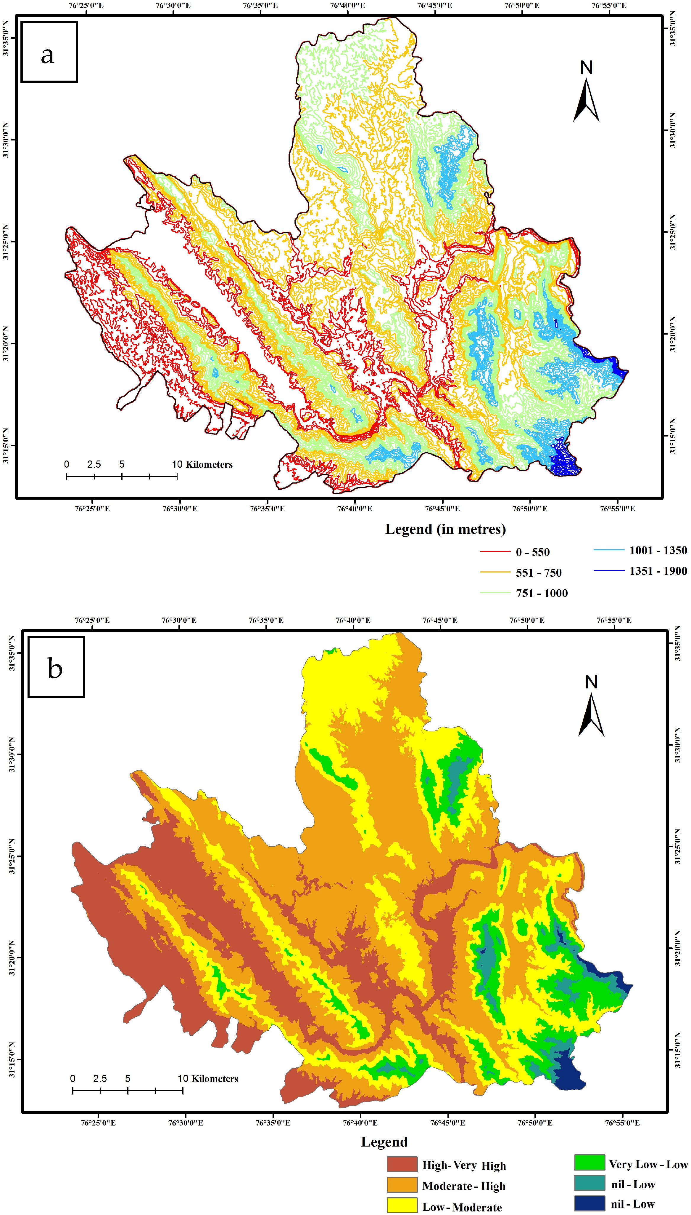
4.6. Elevation Analysis
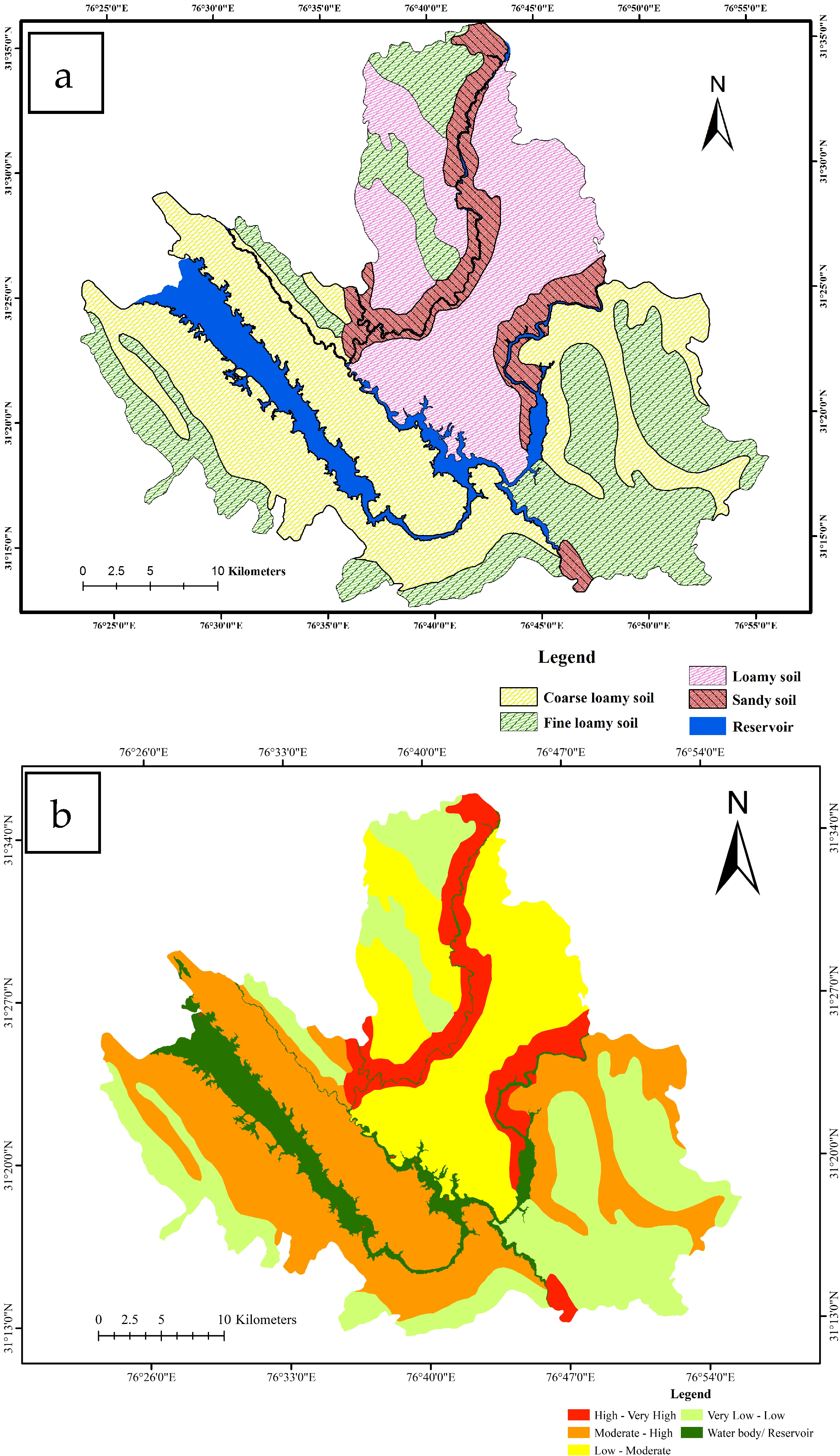
4.7. Soil Analysis
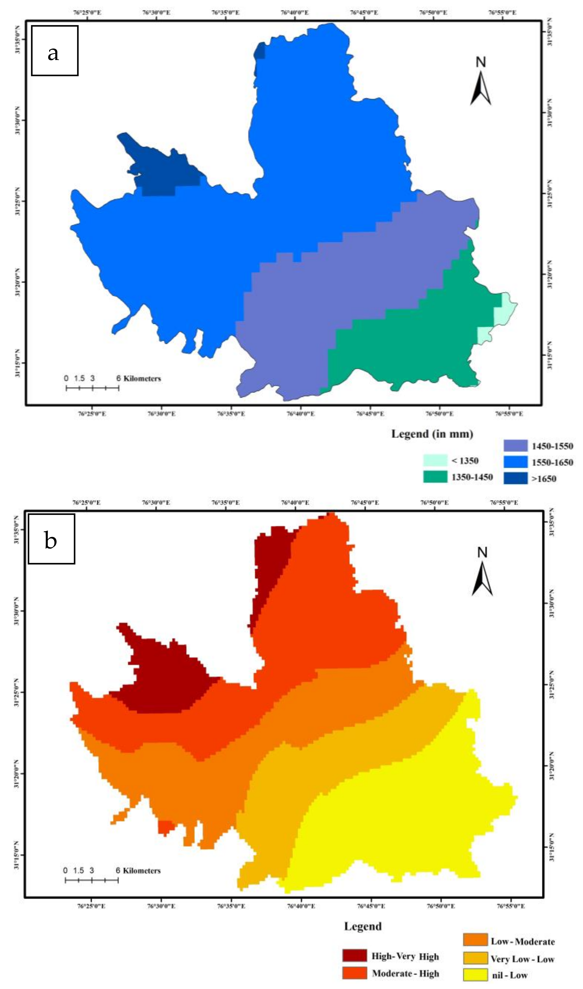
4.8. Rainfall Analysis
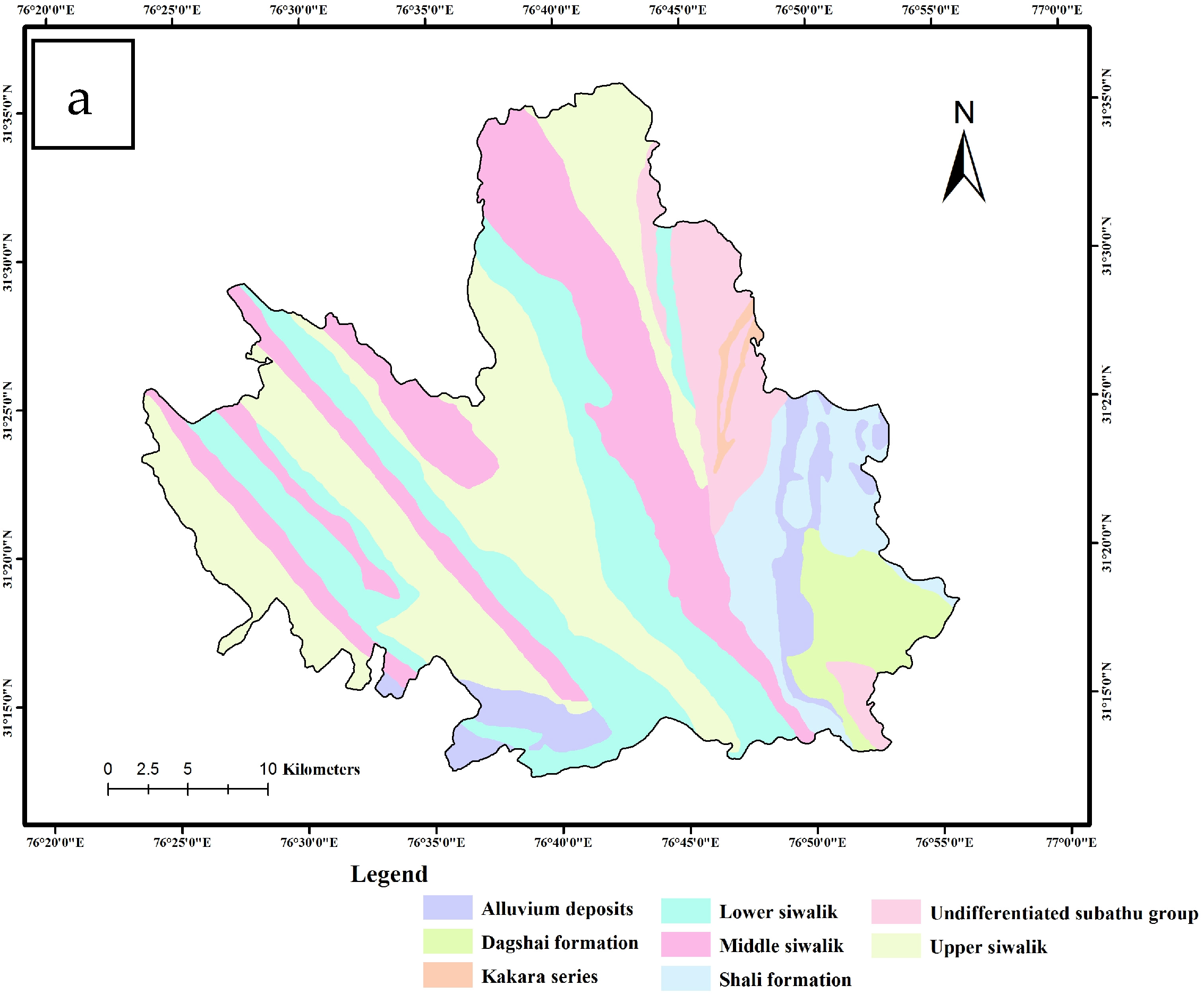
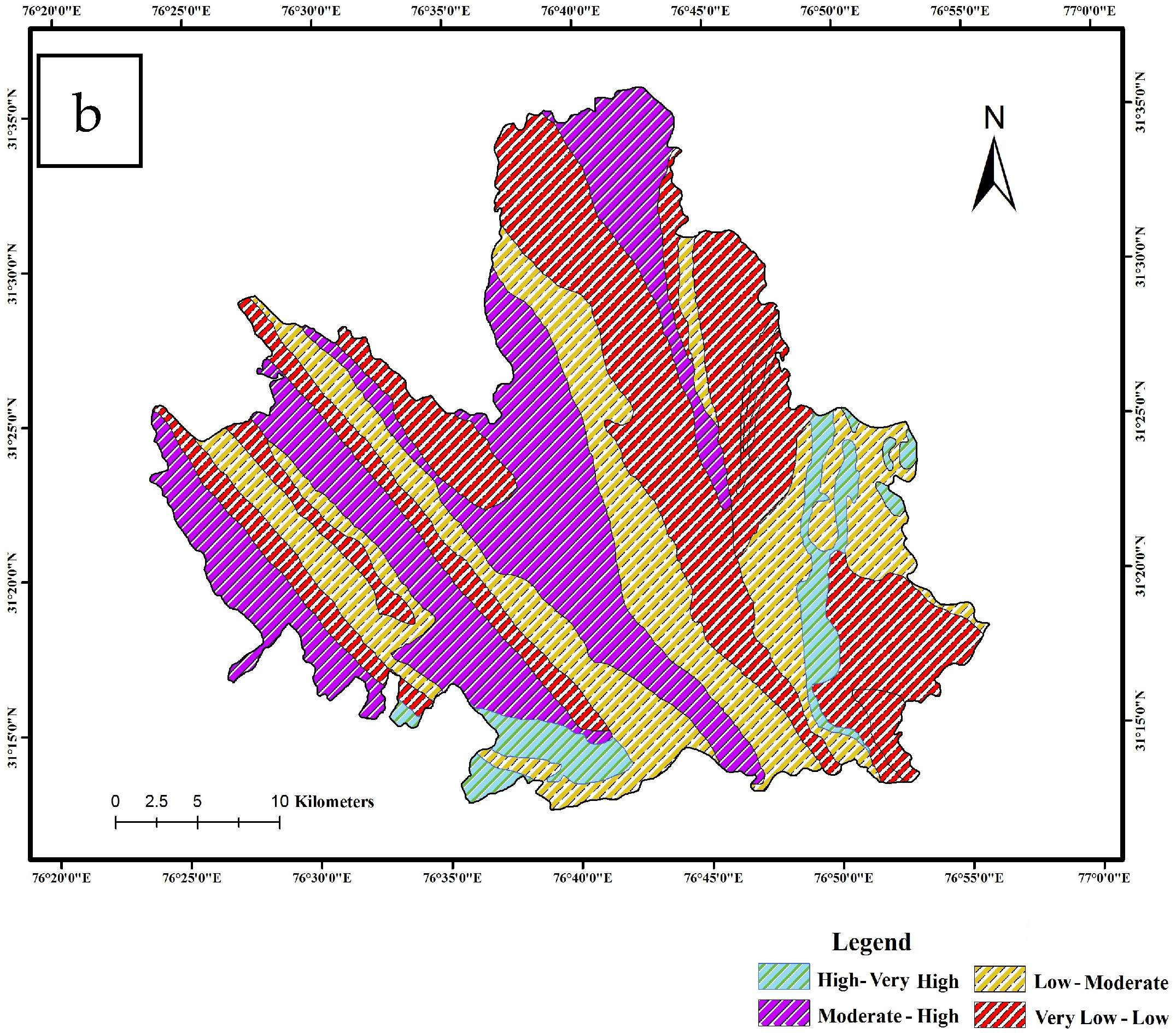
4.9. Lithology Analysis
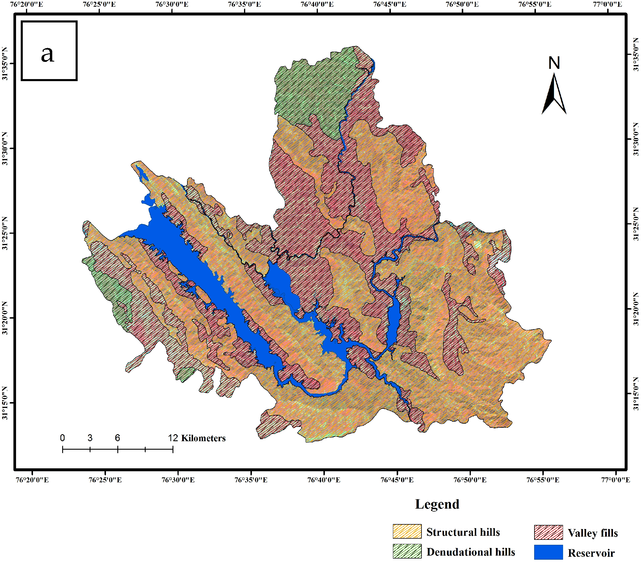
4.10. Geomorpology Analysis
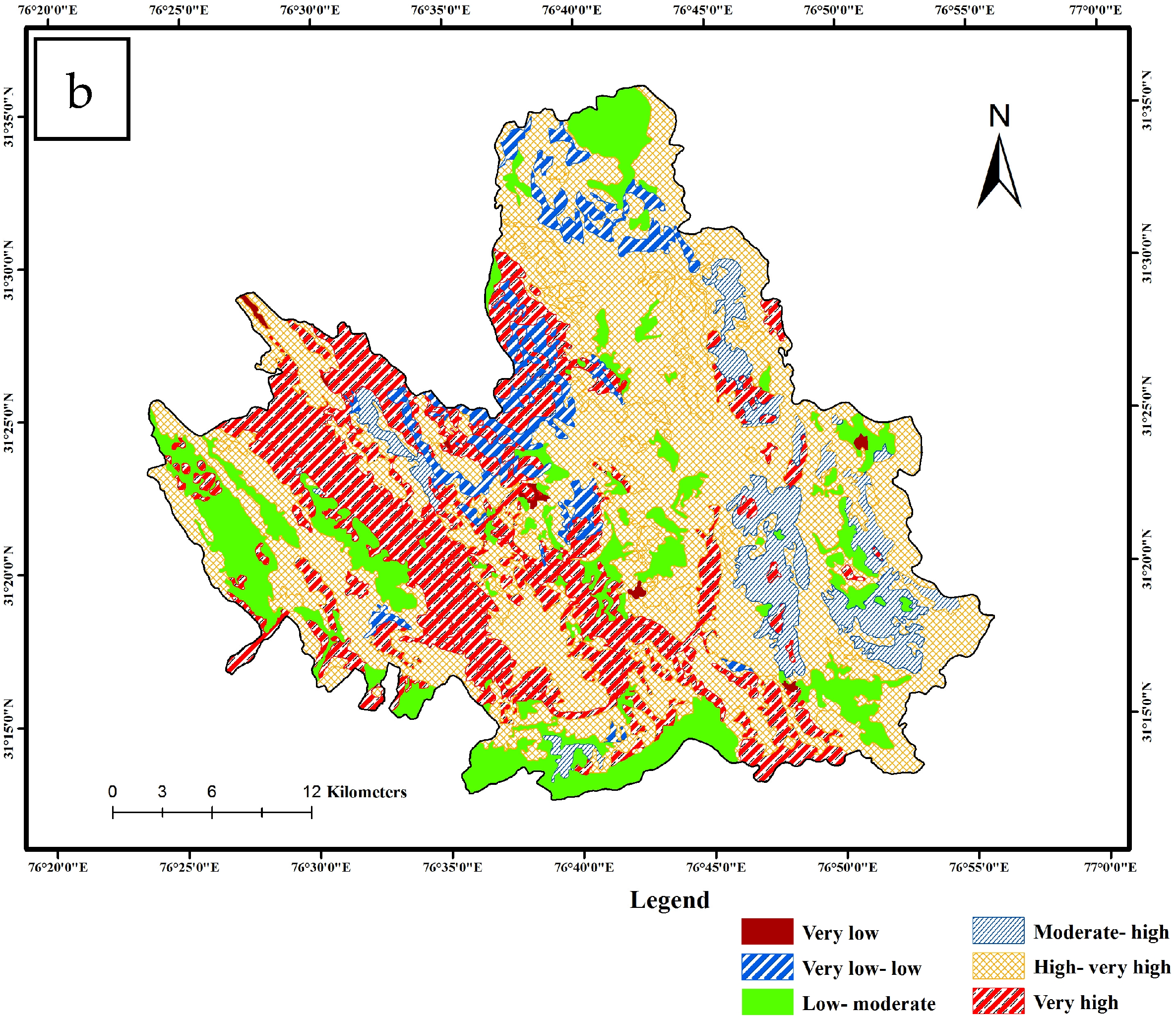
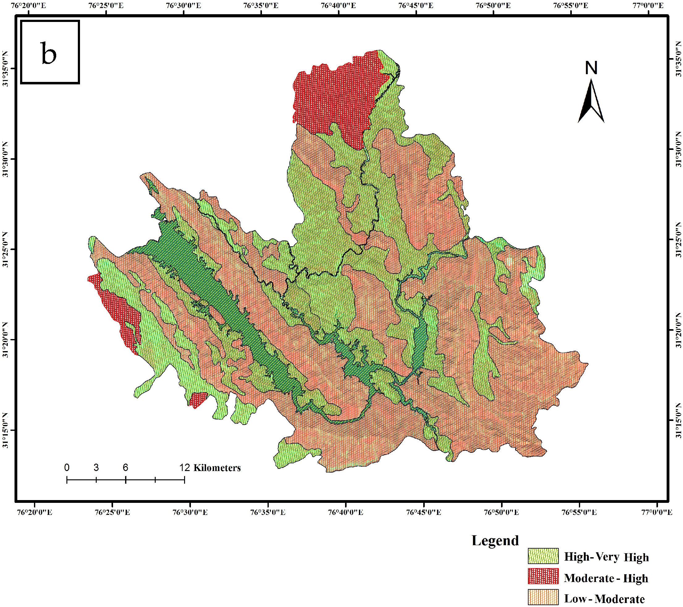
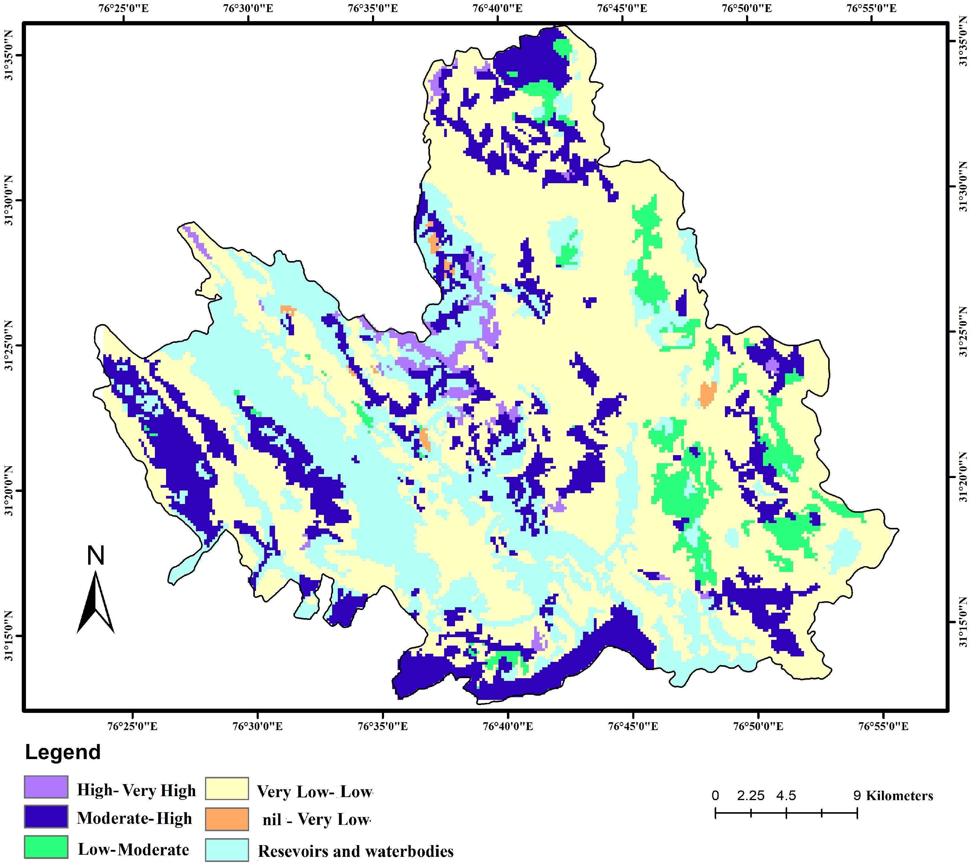
4.11. Delineation of Groundwater Potential Zones
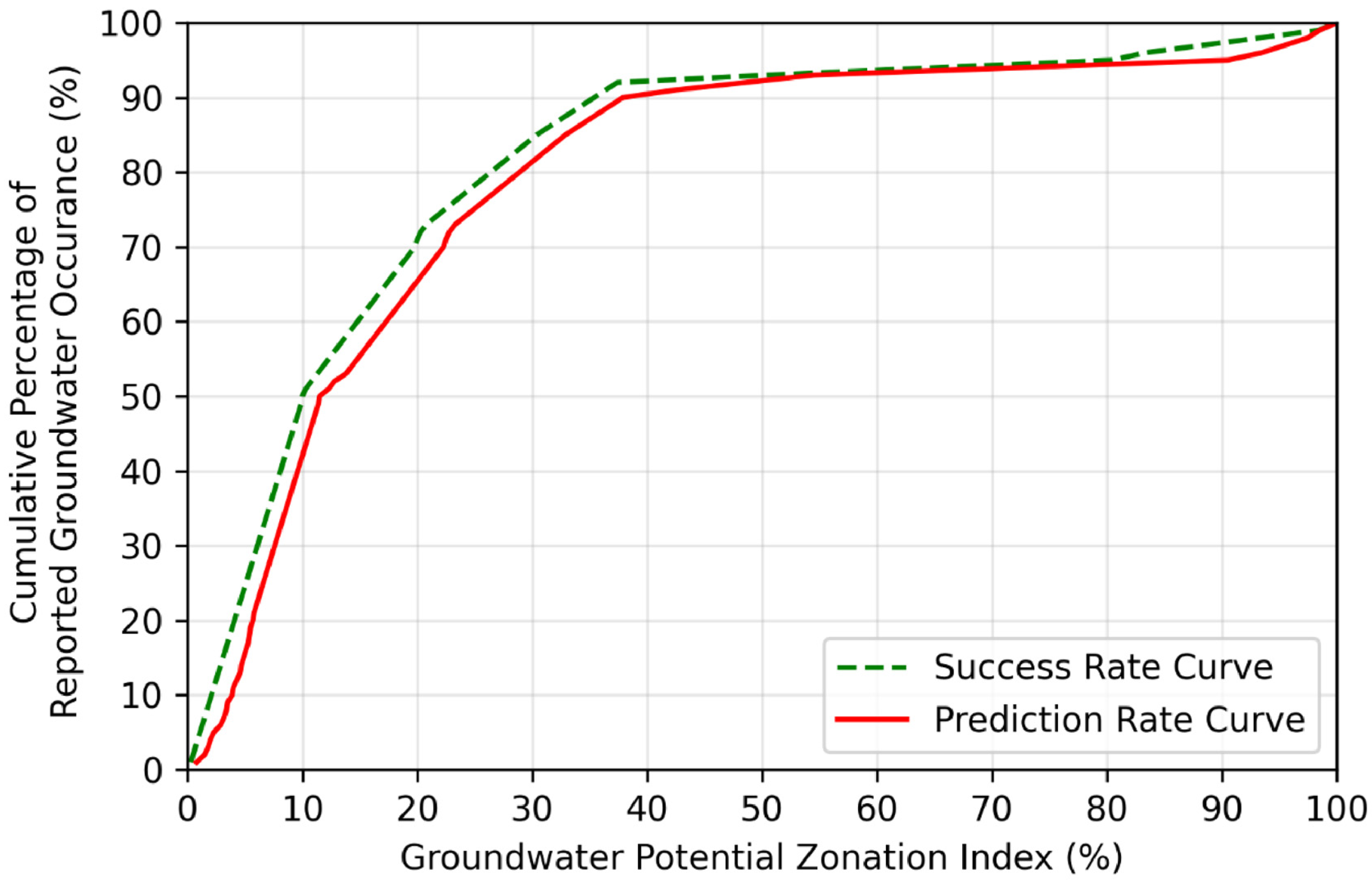
4.12. Validation
5. Conclusions
Author Contributions
Funding
Data Availability Statement
Acknowledgments
Conflicts of Interest
References
- Vereecken, H.; Amelung, W.; Bauke, S.L.; Bogena, H.; Brüggemann, N.; Montzka, C.; Vanderborght, J.; Bechtold, M.; Blöschl, G.; Carminati, A.; et al. Soil hydrology in the Earth system. Nat. Rev. Earth Environ. 2022, 3, 573–587. [Google Scholar] [CrossRef]
- Zhang, K.; Li, H.; Han, J.; Jiang, B.; Gao, J. Understanding of mineral change mechanisms in coal mine groundwater reservoir and their influences on effluent water quality: A experimental study. Int. J. Coal Sci. Technol. 2021, 8, 154–167. [Google Scholar] [CrossRef]
- Chilton, J. Groundwater Pollution—Developments in Water Science. In Water Quality Assessments—A Guide to Use of Biota, Sediments and Water in Environmental Monitoring, 2nd ed.; Chapman and Hall Ltd.: London, UK, 1996; Volume 5, p. 273. [Google Scholar]
- Gibert, O.; Abenza, M.; Reig, M.; Vecino, X.; Sánchez, D.; Arnaldos, M.; Cortina, J.L. Removal of nitrate from groundwater by nano-scale zero-valent iron injection pulses in continuous-flow packed soil columns. Sci. Total Environ. 2022, 810, 152300. [Google Scholar] [CrossRef]
- Harris, S.J.; Cendón, D.I.; Hankin, S.I.; Peterson, M.A.; Xiao, S.; Kelly, B.F. Isotopic evidence for nitrate sources and controls on denitrification in groundwater beneath an irrigated agricultural district. Sci. Total Environ. 2022, 817, 152606. [Google Scholar] [CrossRef]
- Wang, X.; Xu, Y.J.; Zhang, L. Watershed scale spatiotemporal nitrogen transport and source tracing using dual isotopes among surface water, sediments and groundwater in the Yiluo River Watershed, Middle of China. Sci. Total Environ. 2022, 833, 155180. [Google Scholar] [CrossRef] [PubMed]
- Singh, A.P.; Bhakar, P. Development of groundwater sustainability index: A case study of western arid region of Rajasthan, India. Environ. Dev. Sustain. 2021, 23, 1844–1868. [Google Scholar] [CrossRef]
- Kumar, P.; Avtar, R.; Dasgupta, R.; Johnson, B.A.; Mukherjee, A.; Ahsan, M.N.; Nguyen, D.C.; Nguyen, H.Q.; Shaw, R.; Mishra, B.K. Socio-hydrology: A key approach for adaptation to water scarcity and achieving human well-being in large riverine islands. Prog. Disaster Sci. 2020, 8, 100134. [Google Scholar] [CrossRef]
- Shyam, M.; Meraj, G.; Kanga, S.; Farooq, M.; Singh, S.K.; Sahu, N.; Kumar, P. Assessing the Groundwater Reserves of the Udaipur District, Aravalli Range, India, Using Geospatial Techniques. Water 2022, 14, 648. [Google Scholar] [CrossRef]
- Meraj, G. Assessing the Impacts of Climate Change on Ecosystem Service Provisioning in Kashmir Valley India. Ph.D. Thesis, Suresh Gyan Vihar University, Jaipur, India, 2021. [Google Scholar]
- Meraj, G.; Singh, S.K.; Kanga, S.; Islam, M.N. Modeling on comparison of ecosystem services concepts, tools, methods and their ecological-economic implications: A review. Model. Earth Syst. Environ. 2021, 8, 15–34. [Google Scholar] [CrossRef]
- Upadhyay, M.K.; Majumdar, A.; Barla, A.; Bose, S.; Srivastava, S. An assessment of arsenic hazard in groundwater–soil–rice system in two villages of Nadia district, West Bengal, India. Environ. Geochem. Health 2019, 41, 2381–2395. [Google Scholar] [CrossRef]
- Galkate, R.V.; Yadav, S.; Pandey, R.P.; Negm, A.M.; Yadava, R.N. An Overview: Water Resource Management Aspects in India. Water Qual. Assess. Manag. India 2022, 16, 29–55. [Google Scholar]
- Prasad, R.K.; Mondal, N.C.; Banerjee, P.; Nandakumar, M.V.; Singh, V.S. Deciphering Potential Groundwater Zone in Hard Rock through the Application of GIS. Environ. Geol. 2008, 55, 467–475. [Google Scholar] [CrossRef]
- Hamilton, P. Groundwater and Surface Water: A Single Resource. Water Environ. Technol. 2005, 17, 37–41. [Google Scholar]
- Pradhan, B. Groundwater Potential Zonation for Basaltic Watersheds Using Satellite Remote Sensing Data and GIS Techniques. Cent. Eur. J. Geosci. 2009, 1, 120–129. [Google Scholar] [CrossRef]
- Becker, M.W. Potential for Satellite Remote Sensing of Ground Water. Groundwater 2006, 44, 306–318. [Google Scholar] [CrossRef]
- Rodell, M.; Famiglietti, J.S. The Potential for Satellite-Based Monitoring of Groundwater Storage Changes Using GRACE: The High Plains Aquifer, Central US. J. Hydrol. 2002, 263, 245–256. [Google Scholar] [CrossRef] [Green Version]
- Li, W.; Fan, X.; Huang, F.; Chen, W.; Hong, H.; Huang, J.; Guo, Z. Uncertainties analysis of collapse susceptibility prediction based on remote sensing and GIS: Influences of different data-based models and connections between collapses and environmental factors. Remote Sens. 2020, 12, 4134. [Google Scholar] [CrossRef]
- Rather, M.A.; Meraj, G.; Farooq, M.; Shiekh, B.A.; Kumar, P.; Kanga, S.; Singh, S.K.; Sahu, N.; Tiwari, S.P. Identifying the Potential Dam Sites to Avert the Risk of Catastrophic Floods in the Jhelum Basin, Kashmir, NW Himalaya, India. Remote Sens. 2022, 14, 1538. [Google Scholar] [CrossRef]
- Abijith, D.; Saravanan, S.; Singh, L.; Jennifer, J.J.; Saranya, T.; Parthasarathy, K.S.S. GIS-Based Multi-Criteria Analysis for Identification of Potential Groundwater Recharge Zones—A Case Study from Ponnaniyaru Watershed, Tamil Nadu, India. HydroResearch 2020, 3, 1–14. [Google Scholar] [CrossRef]
- Raju, R.S.; Raju, G.S.; Rajasekhar, M. Identification of Groundwater Potential Zones in Mandavi River Basin, Andhra Pradesh, India Using Remote Sensing, GIS and MIF Techniques. HydroResearch 2019, 2, 1–11. [Google Scholar] [CrossRef]
- Ahmed, A.; Ranasinghe-Arachchilage, C.; Alrajhi, A.; Hewa, G. Comparison of Multicriteria Decision-Making Tech-niques for Groundwater Recharge Potential Zonation: Case Study of the Willochra Basin, South Australia. Water 2021, 13, 525. [Google Scholar] [CrossRef]
- Anbarasu, S.; Brindha, K.; Elango, L. Multi-influencing factor method for delineation of groundwater potential zones using remote sensing and GIS techniques in the western part of Perambalur district, southern India. Earth Sci. Inform. 2020, 13, 317–332. [Google Scholar] [CrossRef]
- Roy, S.; Hazra, S.; Chanda, A.; Das, S. Assessment of Groundwater Potential Zones Using Multi-Criteria Deci-sion-Making Technique: A Micro-Level Case Study from Red and Lateritic Zone (RLZ) of West Bengal, India. Sustain. Water Resour. Manag. 2020, 6, 4. [Google Scholar] [CrossRef]
- Pourghasemi, H.R.; Beheshtirad, M. Assessment of a Data-Driven Evidential Belief Function Model and GIS for Groundwater Potential Mapping in the Koohrang Watershed, Iran. Geocarto Int. 2015, 30, 662–685. [Google Scholar] [CrossRef]
- Sander, P. Lineaments in Groundwater Exploration: A Review of Applications and Limitations. Hydrogeol. J. 2007, 15, 71–74. [Google Scholar] [CrossRef]
- Nag, S.K.; Ray, S. Deciphering Groundwater Potential Zones Using Geospatial Technology: A Study in Bankura Block I and Block II, Bankura District, West Bengal. Arab. J. Sci. Eng. 2015, 40, 205–214. [Google Scholar] [CrossRef]
- Singh, D.K.; Singh, A.K. Groundwater Situation in India: Problems and Perspective. Int. J. Water Resour. Dev. 2002, 18, 563–580. [Google Scholar] [CrossRef]
- Singh, L.K.; Jha, M.K.; Chowdary, V.M. Assessing the Accuracy of GIS-Based Multi-Criteria Decision Analysis Ap-proaches for Mapping Groundwater Potential. Ecol. Indic. 2018, 91, 24–37. [Google Scholar] [CrossRef]
- Thapa, R.; Gupta, S.; Guin, S.; Kaur, H. Assessment of Groundwater Potential Zones Using Multi-Influencing Factor (MIF) and GIS: A Case Study from Birbhum District, West Bengal. Appl. Water Sci. 2017, 7, 4117–4131. [Google Scholar] [CrossRef]
- Fagbohun, B.J. Integrating GIS and Multi-Influencing Factor Technique for Delineation of Potential Groundwater Recharge Zones in Parts of Ilesha Schist Belt, Southwestern Nigeria. Environ. Earth Sci. 2018, 77, 69. [Google Scholar] [CrossRef]
- Oikonomidis, D.; Dimogianni, S.; Kazakis, N.; Voudouris, K. A GIS/Remote Sensing-Based Methodology for Groundwater Potentiality Assessment in Tirnavos Area, Greece. J. Hydrol. 2015, 525, 197–208. [Google Scholar] [CrossRef]
- Owolabi, S.T.; Madi, K.; Kalumba, A.M.; Orimoloye, I.R. A Groundwater Potential Zone Mapping Approach for Semi-Arid Environments Using Remote Sensing (RS), Geographic Information System (GIS), and Analytical Hierarchical Process (AHP) Techniques: A Case Study of Buffalo Catchment, Eastern Cape, South Africa. Arab. J. Geosci. 2020, 13, 1184. [Google Scholar] [CrossRef]
- Tolche, A.D. Groundwater Potential Mapping Using Geospatial Techniques: A Case Study of Dhungeta-Ramis Sub-Basin, Ethiopia. Geol. Ecol. Landsc. 2021, 5, 65–80. [Google Scholar] [CrossRef]
- Yeh, H.F.; Cheng, Y.S.; Lin, H.I.; Lee, C.H. Mapping Groundwater Recharge Potential Zone Using a GIS Approach in Hualian River, Taiwan. Sustain. Environ. Res. 2016, 26, 33–43. [Google Scholar] [CrossRef] [Green Version]
- Zghibi, A.; Mirchi, A.; Msaddek, M.H.; Merzougui, A.; Zouhri, L.; Taupin, J.D.; Chekirbane, A.; Chenini, I.; Tarhouni, J. Using Analytical Hierarchy Process and Multi-Influencing Factors to Map Groundwater Recharge Zones in a Semi-Arid Mediterranean. Water 2020, 12, 2525. [Google Scholar] [CrossRef]
- Pradhan, A.M.; Kim, Y.T.; Shrestha, S.; Huynh, T.C.; Nguyen, B.P. Application of deep neural network to capture groundwater potential zone in mountainous terrain, Nepal Himalaya. Environ. Sci. Pollut. Res. 2021, 28, 18501–18517. [Google Scholar] [CrossRef] [PubMed]
- Nasir, M.J.; Khan, S.; Ayaz, T.; Khan, A.Z.; Ahmad, W.; Lei, M. An Integrated Geospatial Multi-Influencing Factor Approach to Delineate and Identify Groundwater Potential Zones in Kabul Province, Afghanistan. Environ. Earth Sci. 2021, 80, 453. [Google Scholar] [CrossRef]
- Jhariya, D.C.; Kumar, T.; Gobinath, M.; Diwan, P.; Kishore, N. Assessment of Groundwater Potential Zone Using Remote Sensing, GIS and Multi Criteria Decision Analysis Techniques. J. Geol. Soc. India 2016, 88, 481–492. [Google Scholar] [CrossRef]
- Magesh, N.S.; Chandrasekar, N.; Soundranayagam, J.P. Delineation of Groundwater Potential Zones in Theni District, Tamil Nadu, Using Remote Sensing, GIS and MIF Techniques. Geosci. Front. 2012, 3, 189–196. [Google Scholar] [CrossRef] [Green Version]
- Arkoprovo, B.; Adarsa, J.; Animesh, M. Application of Remote Sensing, GIS and MIF Technique for Elucidation of Groundwater Potential Zones from a Part of Orissa Coastal Tract, Eastern India. Res. J. Recent Sci. 2013, 2, 42–49. [Google Scholar]
- Bhattacharya, S.; Das, S.; Das, S.; Kalashetty, M.; Warghat, S.R. An Integrated Approach for Mapping Groundwater Potential Applying Geospatial and MIF Techniques in the Semiarid Region. Environ. Dev. Sustain. 2021, 23, 495–510. [Google Scholar] [CrossRef]
- Das, S.; Gupta, A.; Ghosh, S. Exploring Groundwater Potential Zones Using MIF Technique in Semi-Arid Region: A Case Study of Hingoli District, Maharashtra. Spat. Inf. Res. 2017, 25, 749–756. [Google Scholar] [CrossRef]
- Bhuvaneswaran, C.; Ganesh, A.; Nevedita, S. Spatial Analysis of Groundwater Potential Zones Using Remote Sensing, GIS and MIF Techniques in Uppar Odai Sub-Watershed, Nandiyar, Cauvery Basin, Tamilnadu. Int. J. Curr. Res. 2015, 7, 20765–20774. [Google Scholar]
- Singha, S.; Pasupuleti, S.; Durbha, K.S.; Singha, S.S.; Singh, R.; Venkatesh, A.S. An analytical hierarchy process-based geospatial modeling for delineation of potential anthropogenic contamination zones of groundwater from Arang block of Raipur district, Chhattisgarh, Central India. Environ. Earth Sci. 2019, 78, 1–9. [Google Scholar] [CrossRef]
- Dwivedi, C.S.; Raza, R.; Mitra, D.; Pandey, A.C.; Jhariya, D.C. Groundwater potential zone delineation in hard rock terrain for sustainable groundwater development and management in South Madhya Pradesh, India. Geogr. Environ. Sustain. 2021, 14, 106–121. [Google Scholar] [CrossRef]
- Sud, A. Delineation of Groundwater Potential Zone Using the Integration of Geospatial Model and Multi Influencing Factor (MIF) Decision Making Technique: A Review. SGVU J. Clim. Chang. Water 2021, 8, 1–13. [Google Scholar]
- Kumar, S.; Shruti, S.; Shailja, K.; Mishra, K. Delineation of Groundwater Potential Zone Using Geospatial Techniques for Shimla City, Himachal Pradesh (India). Int. J. Sci. Res. Dev. 2017, 5, 225–234. [Google Scholar]
- Chauhan, N.S. Medicinal and Aromatic Plants of Himachal Pradesh; Indus Publishing: New Delhi, India, 1999. [Google Scholar]
- Upgupta, S.; Sharma, J.; Jayaraman, M.; Kumar, V.; Ravindranath, N.H. Climate change impact and vulnerability assessment of forests in the Indian Western Himalayan region: A case study of Himachal Pradesh, India. Clim. Risk Manag. 2015, 10, 63–67. [Google Scholar] [CrossRef] [Green Version]
- Prasher, R.S.; Devi, N. Agricultural diversification in Himachal Pradesh: An economic analysis. Indian J. Econ. Dev. 2018, 6, 1–6. [Google Scholar]
- Dev, R.; Bali, M. Evaluation of groundwater quality and its suitability for drinking and agricultural use in district Kangra of Himachal Pradesh, India. J. Saudi Soc. Agric. Sci. 2019, 18, 462–468. [Google Scholar] [CrossRef]
- Parihar, S. Salvaging, Transplantation and Reconstruction of Heritage Sites, Techniques and Problems: A Study of the Submerged Temple of Bilaspur District in Himachal Pradesh. Indian Hist. Rev. 2019, 46, 167–183. [Google Scholar] [CrossRef]
- Singh, S.; Dhasmana, M.K.; Shrivastava, V.; Sharma, V.; Pokhriyal, N.; Thakur, P.K.; Aggarwal, S.P.; Nikam, B.R.; Garg, V.; Chouksey, A.; et al. Estimation of revised capacity in Gobind Sagar reservoir using Google earth engine and GIS. Int. Arch. Photogramm. Remote Sens. Spat. Inf. Sci. 2018, 42. [Google Scholar] [CrossRef] [Green Version]
- Kanga, S.; Singh, S.K.; Meraj, G.; Kumar, A.; Parveen, R.; Kranjčić, N.; Đurin, B. Assessment of the impact of urbanization on geoenvironmental settings using geospatial techniques: A study of Panchkula District, Haryana. Geographies 2022, 2, 1–10. [Google Scholar] [CrossRef]
- Hudson, P.F.; Colditz, R.R.; Aguilar-Robledo, M. Spatial relations between floodplain environments and land use–land cover of a large lowland tropical river valley: Panuco basin, Mexico. Environ. Manag. 2006, 38, 487–503. [Google Scholar] [CrossRef] [PubMed]
- Meraj, G.; Farooq, M.; Singh, S.K.; Islam, M.N.; Kanga, S. Modeling the sediment retention and ecosystem provisioning services in the Kashmir valley, India, Western Himalayas. Model. Earth Syst. Environ. 2022, 8, 3859–3884. [Google Scholar] [CrossRef]
- Lahon, D.; Sahariah, D.; Debnath, J.; Nath, N.; Meraj, G.; Farooq, M.; Kanga, S.; Singh, S.; Chand, K. Growth of water hyacinth biomass and its impact on the floristic composition of aquatic plants in a wetland ecosystem of the Brahmaputra floodplain of Assam, India. PeerJ 2023, 11, e14811. [Google Scholar] [CrossRef]
- Nath, N.; Sahariah, D.; Meraj, G.; Debnath, J.; Kumar, P.; Lahon, D.; Chand, K.; Farooq, M.; Chandan, P.; Singh, S.K.; et al. Land Use and Land Cover Change Monitoring and Prediction of a UNESCO World Heritage Site: Kaziranga Eco-Sensitive Zone Using Cellular Automata-Markov Model. Land 2023, 12, 151. [Google Scholar] [CrossRef]
- Kanga, S.; Meraj, G.; Johnson, B.A.; Singh, S.K.; PV, M.N.; Farooq, M.; Kumar, P.; Marazi, A.; Sahu, N. Understanding the Linkage between Urban Growth and Land Surface Temperature—A Case Study of Bangalore City, India. Remote Sens. 2022, 14, 4241. [Google Scholar] [CrossRef]
- Meraj, G.; Romshoo, S.A.; Yousuf, A.R.; Altaf, S.; Altaf, F. Assessing the influence of watershed characteristics on the flood vulnerability of Jhelum basin in Kashmir Himalaya. Nat. Hazards 2015, 77, 153–175. [Google Scholar] [CrossRef]
- Masoud, A.; Koike, K. Applicability of computer-aided comprehensive tool (LINDA: Lineament Detection and Analysis) and shaded digital elevation model for characterizing and interpreting morphotectonic features from lineaments. Comput. Geosci. 2017, 106, 89–100. [Google Scholar] [CrossRef]
- Soliman, A.; Han, L. Effects of vertical accuracy of digital elevation model (DEM) data on automatic lineaments extraction from shaded DEM. Adv. Space Res. 2019, 64, 603–622. [Google Scholar] [CrossRef]
- Altaf, F.; Meraj, G.; Romshoo, S.A. Morphometric analysis to infer hydrological behaviour of Lidder watershed, Western Himalaya, India. Geogr. J. 2013, 2013, 178021. [Google Scholar] [CrossRef] [Green Version]
- Meraj, G.; Yousuf, A.R.; Romshoo, S.A. Impacts of the Geo-Environmental Setting on the Flood Vulnerability at Watershed Scale in the Jhelum Basin. Master’s Thesis, University of Kashmir, Srinagar, India, 2013. [Google Scholar]
- Altaf, S.; Meraj, G.; Romshoo, S.A. Morphometry and land cover based multi-criteria analysis for assessing the soil erosion susceptibility of the western Himalayan watershed. Environ. Monit. Assess. 2014, 186, 8391–8412. [Google Scholar] [CrossRef] [PubMed]
- Ollier, C.D.; Thomasson, A.J. Asymmetrical valleys of the Chiltern Hills. Geogr. J. 1957, 123, 71–80. [Google Scholar] [CrossRef]
- Jackson, M.; Roering, J.J. Post-fire geomorphic response in steep, forested landscapes: Oregon Coast Range, USA. Quat. Sci. Rev. 2009, 28, 1131–1146. [Google Scholar] [CrossRef]
- Debnath, J.; Meraj, G.; Das Pan, N.; Chand, K.; Debbarma, S.; Sahariah, D.; Gualtieri, C.; Kanga, S.; Singh, S.K.; Farooq, M.; et al. Integrated remote sensing and field-based approach to assess the temporal evolution and future projection of meanders: A case study on River Manu in North-Eastern India. PLoS ONE 2022, 17, e0271190. [Google Scholar] [CrossRef]
- Roy, P.K.; Basak, S.K.; Mohinuddin, S.; Roy, M.B.; Halder, S.; Ghosh, T. Modelling groundwater potential zone using fuzzy logic and geospatial technology of an deltaic island. Model. Earth Syst. Environ. 2022, 8, 5565–5584. [Google Scholar] [CrossRef]
- Navale, V.; Mhaske, S. Artificial Neural Network (ANN) and Adaptive Neuro-Fuzzy Inference System (ANFIS) model for Forecasting Groundwater Level in the Pravara River Basin, India. Model. Earth Syst. Environ. 2022, 27, 1–4. [Google Scholar] [CrossRef]
- Wirth, S.B.; Carlier, C.; Cochand, F.; Hunkeler, D.; Brunner, P. Lithological and tectonic control on groundwater contribution to stream discharge during low-flow conditions. Water 2020, 12, 821. [Google Scholar] [CrossRef] [Green Version]
- Singh, M.; Hartsch, K. Basics of soil erosion. In Watershed Hydrology, Management and Modeling; CRC Press: Boca Raton, FL, USA, 2019; Volume 31, pp. 1–61. [Google Scholar]
- Misra, D.K.; Tewari, V.C. Tectonics and sedimentation of the rocks between Mandi and Rohtang, Beas valley, Himachal Pradesh, India. Geosci. J. 1988, 9, 153–172. [Google Scholar]
- Srivastava, P.; Patel, S.; Singh, N.; Jamir, T.; Kumar, N.; Aruche, M.; Patel, R.C. Early Oligocene paleosols of the Dagshai Formation, India: A record of the oldest tropical weathering in the Himalayan foreland. Sediment. Geol. 2013, 294, 142–156. [Google Scholar] [CrossRef]
- Rahimi-Aghdam, S.; Chau, V.T.; Lee, H.; Nguyen, H.; Li, W.; Karra, S.; Rougier, E.; Viswanathan, H.; Srinivasan, G.; Bažant, Z.P. Branching of hydraulic cracks enabling permeability of gas or oil shale with closed natural fractures. Proc. Natl. Acad. Sci. USA 2019, 116, 1532–1537. [Google Scholar] [CrossRef] [PubMed] [Green Version]
- Grenfell, S.; Grenfell, M.; Ellery, W.; Job, N.; Walters, D. A genetic geomorphic classification system for southern African palustrine wetlands: Global implications for the management of wetlands in drylands. Front. Environ. Sci. 2019, 7, 174. [Google Scholar] [CrossRef] [Green Version]
- Roy, S.; Bose, A.; Mandal, G. Modeling and mapping geospatial distribution of groundwater potential zones in Darjeeling Himalayan region of India using analytical hierarchy process and GIS technique. Model. Earth Syst. Environ. 2022, 8, 1563–1584. [Google Scholar] [CrossRef]
- Meraj, G.; Romshoo, S.A.; Ayoub, S.; Altaf, S. Geoinformatics based approach for estimating the sediment yield of the mountainous watersheds in Kashmir Himalaya, India. Geocarto Int. 2018, 33, 1114–1138. [Google Scholar] [CrossRef]
- Fayaz, M.; Meraj, G.; Khader, S.A.; Farooq, M. ARIMA and SPSS statistics based assessment of landslide occurrence in western Himalayas. Environ. Chall. 2022, 9, 100624. [Google Scholar] [CrossRef]
- Fayaz, M.; Meraj, G.; Khader, S.A.; Farooq, M.; Kanga, S.; Singh, S.K.; Kumar, P.; Sahu, N. Management of landslides in a rural–urban transition zone using machine learning algorithms—A case study of a National Highway (NH-44), India, in the Rugged Himalayan Terrains. Land 2022, 11, 884. [Google Scholar] [CrossRef]
- Rehman, A.; Song, J.; Haq, F.; Mahmood, S.; Ahamad, M.I.; Basharat, M.; Sajid, M.; Mehmood, M.S. Multi-hazard susceptibility assessment using the analytical hierarchy process and frequency ratio techniques in the Northwest Himalayas, Pakistan. Remote Sens. 2022, 14, 554. [Google Scholar] [CrossRef]
- Islam, F.; Ahmad, M.N.; Janjuhah, H.T.; Ullah, M.; Islam, I.U.; Kontakiotis, G.; Skilodimou, H.D.; Bathrellos, G.D. Modelling and Mapping of Soil Erosion Susceptibility of Murree, Sub-Himalayas Using GIS and RS-Based Models. Appl. Sci. 2022, 12, 12211. [Google Scholar] [CrossRef]
- Post, D.E.; Votta, L.G. Computational science demands a new paradigm. Phys. Today 2005, 58, 35–41. [Google Scholar] [CrossRef]
- Rasha, K.M. Salinity Prediction at the Bhairab River in the South-Western Part of Bangladesh Using Artificial Neural Network. Nat. Environ. Pollut. Technol. 2022, 21, 1431–1438. [Google Scholar] [CrossRef]
- Wang, G.; Chen, X.; Chen, W. Spatial prediction of landslide susceptibility based on GIS and discriminant functions. ISPRS Int. J. Geo Inf. 2020, 9, 144. [Google Scholar] [CrossRef] [Green Version]
- Yi, Y.; Zhang, Z.; Zhang, W.; Jia, H.; Zhang, J. Landslide susceptibility mapping using multiscale sampling strategy and convolutional neural network: A case study in Jiuzhaigou region. Catena 2020, 195, 104851. [Google Scholar] [CrossRef]
- Arabameri, A.; Saha, S.; Chen, W.; Roy, J.; Pradhan, B.; Bui, D.T. Flash flood susceptibility modelling using functional tree and hybrid ensemble techniques. J. Hydrol. 2020, 587, 125007. [Google Scholar] [CrossRef]
- Chen, Z.; Song, D.; Juliev, M.; Pourghasemi, H.R. Landslide susceptibility mapping using statistical bivariate models and their hybrid with normalized spatial-correlated scale index and weighted calibrated landslide potential model. Environ. Earth Sci. 2021, 80, 1–9. [Google Scholar] [CrossRef]
- Lee, S.; Hong, S.M.; Jung, H.S. GIS-Based Groundwater Potential Mapping Using Artificial Neural Network and Support Vector Machine Models: The Case of Boryeong City in Korea. Geocarto Int. 2018, 33, 847–861. [Google Scholar] [CrossRef]
- Sener, E.; Davraz, A.; Ozcelik, M. An Integration of GIS and Remote Sensing in Groundwater Investigations: A Case Study in Burdur, Turkey. Hydrogeol. J. 2005, 13, 826–834. [Google Scholar] [CrossRef]
- Arulbalaji, P.; Padmalal, D.; Sreelash, K. GIS and AHP Techniques Based Delineation of Groundwater Potential Zones: A Case Study from Southern Western Ghats, India. Sci. Rep. 2019, 9, 2082. [Google Scholar] [CrossRef] [Green Version]
- Sashikkumar, M.C.; Selvam, S.; Kalyanasundaram, V.L.; Johnny, J.C. GIS Based Groundwater Modeling Study to Assess the Effect of Artificial Recharge: A Case Study from Kodaganar River Basin, Dindigul District, Tamil Nadu. J. Geol. Soc. India 2017, 89, 57–64. [Google Scholar] [CrossRef]
- Lee, S.; Hyun, Y.; Lee, S.; Lee, M.J. Groundwater potential mapping using remote sensing and GIS-based machine learning techniques. Remote Sens. 2020, 12, 1200. [Google Scholar] [CrossRef] [Green Version]
- Mandal, U.; Sahoo, S.; Munusamy, S.B.; Dhar, A.; Panda, S.N.; Kar, A.; Mishra, P.K. Delineation of Groundwater Potential Zones of Coastal Groundwater Basin Using Multi-Criteria Decision Making Technique. Water Resour. Manag. 2016, 30, 4293–4310. [Google Scholar] [CrossRef]
- Selvarani, A.G.; Elangovan, K.; Kumar, C.S. Evaluation of Groundwater Potential Zones Using Electrical Resistivity and GIS in Noyyal River Basin, Tamil Nadu. J. Geol. Soc. India 2016, 87, 573–582. [Google Scholar] [CrossRef]


| Factor | Major Effect (G) | Minor Effect (H) | Proposed Relative Rates (G + H) | Proposed Score of Each Influencing Factor |
|---|---|---|---|---|
| Drainage Density | 2 | 1 | 3 | 13 |
| Lineament Density | 2 | 0.5 | 2.5 | 11 |
| LULC | 1 | 0.5 | 1.5 | 6 |
| Aspect | 1 | 0 | 1 | 4 |
| Slope | 1 | 1 | 2 | 9 |
| Elevation | 2 | 0.5 | 2.5 | 11 |
| Soil | 1 | 0.5 | 1.5 | 7 |
| Rainfall | 2 | 0.5 | 2.5 | 11 |
| Lithology | 2 | 1 | 3 | 13 |
| Geomorphology | 3 | 0.5 | 3.5 | 15 |
| Total | 23 | 100 |
| Factor | Descriptive Scale | Weight (a) 1–10 | Domain of Effect | Rate (b) 1–4 | Weighted Rating (a × b) | Total | Average Weight (a × b/∑a × b) × 100 |
|---|---|---|---|---|---|---|---|
| Drainage density | <0.5 | 9 | HVH | 3 | 27 | 75 | 11 |
| 0.5–1.0 | 7 | MH | 21 | ||||
| 1.0–1.5 | 5 | LM | 15 | ||||
| 1.5–2.0 | 3 | VLL | 9 | ||||
| >2.0 | 1 | NVL | 3 | ||||
| Lineament density | <0.3 | 1 | NVL | 2.5 | 2.5 | 62.5 | 9 |
| 0.3–0.6 | 3 | VLL | 7.5 | ||||
| 0.6–0.9 | 5 | LM | 12.5 | ||||
| 0.9–1.2 | 7 | MH | 17.5 | ||||
| >1.2 | 9 | HVH | 22.5 | ||||
| LU/LC | Waterbody | 9 | HVH | 1.5 | 13.5 | 81 | 11 |
| Cropland | 9 | HVH | 13.5 | ||||
| Forest Evergreen | 7 | MH | 10.5 | ||||
| Forest Scrub | 7 | MH | 10.5 | ||||
| Forest Deciduous | 7 | MH | 10.5 | ||||
| Grazing land | 6 | MH | 9 | ||||
| Scrubland | 4 | LM | 6 | ||||
| Ravenous land | 3 | VLL | 4.5 | ||||
| Built-up Land | 2 | VLL | 3 | ||||
| Aspect | North | 9 | HVH | 1 | 9 | 44 | 6 |
| North-east | 8 | HVH | 8 | ||||
| East | 7 | MH | 7 | ||||
| North-west | 6 | MH | 6 | ||||
| West | 4 | LM | 4 | ||||
| South-east | 5 | LM | 5 | ||||
| South-west | 3 | VLL | 3 | ||||
| South | 2 | VLL | 2 | ||||
| Flat | 1 | NVL | 1 | ||||
| Slope (degree) | <10 | 9 | HVH | 2 | 18 | 62 | 9 |
| 10–20 | 7 | MH | 14 | ||||
| 20–30 | 6 | MH | 12 | ||||
| 30–40 | 5 | LM | 10 | ||||
| 40–50 | 3 | VLL | 6 | ||||
| >50 | 1 | NVL | 2 | ||||
| Elevation (meters) | <550 | 9 | HVH | 2.5 | 22.5 | 75 | 11 |
| 550–750 | 7 | MH | 17.5 | ||||
| 750–950 | 6 | MH | 15 | ||||
| 950–1150 | 5 | LM | 10 | ||||
| 1150–1350 | 3 | LLV | 7.5 | ||||
| >1350 | 1 | NVL | 2.5 | ||||
| Soil | Sandy | 9 | HVH | 1.5 | 13.5 | 34.5 | 5 |
| Coarse loamy | 7 | MH | 10.5 | ||||
| Loamy | 5 | LM | 7.5 | ||||
| Fine loamy | 2 | VLL | 3 | ||||
| Rainfall (mm) | <1350 | 2 | NVL | 2.5 | 5 | 64.5 | 9 |
| 1350–1450 | 3 | VLL | 7.5 | ||||
| 1450–1550 | 5 | LM | 12 | ||||
| 1550–1650 | 7 | MH | 17.5 | ||||
| >1650 | 9 | HVH | 22.5 | ||||
| Lithology | Alluvium deposit | 9 | HVH | 3 | 27 | 114 | 16 |
| Upper Shiwalik | 7 | MH | 21 | ||||
| Lower Shiwalik | 5 | LM | 15 | ||||
| Shali | 5 | LM | 15 | ||||
| UndifferentialSubathu | 3 | VLL | 9 | ||||
| Middle Shiwalik | 3 | VLL | 9 | ||||
| Dagshai formation | 3 | VLL | 9 | ||||
| Kakara formation | 3 | VLL | 9 | ||||
| Geomorphology | Structural hills | 3 | VLL | 3.5 | 10.5 | 92.5 | 13 |
| Denudational hill | 6 | LM | 19 | ||||
| Valley fill | 9 | HVH | 31.5 | ||||
| Reservoir | 9 | HVH | 31.5 |
Disclaimer/Publisher’s Note: The statements, opinions and data contained in all publications are solely those of the individual author(s) and contributor(s) and not of MDPI and/or the editor(s). MDPI and/or the editor(s) disclaim responsibility for any injury to people or property resulting from any ideas, methods, instructions or products referred to in the content. |
© 2023 by the authors. Licensee MDPI, Basel, Switzerland. This article is an open access article distributed under the terms and conditions of the Creative Commons Attribution (CC BY) license (https://creativecommons.org/licenses/by/4.0/).
Share and Cite
Sud, A.; Kanga, R.; Singh, S.K.; Meraj, G.; Kanga, S.; Kumar, P.; Ramanathan, A.; Sudhanshu; Bhardwaj, V. Simulating Groundwater Potential Zones in Mountainous Indian Himalayas—A Case Study of Himachal Pradesh. Hydrology 2023, 10, 65. https://doi.org/10.3390/hydrology10030065
Sud A, Kanga R, Singh SK, Meraj G, Kanga S, Kumar P, Ramanathan A, Sudhanshu, Bhardwaj V. Simulating Groundwater Potential Zones in Mountainous Indian Himalayas—A Case Study of Himachal Pradesh. Hydrology. 2023; 10(3):65. https://doi.org/10.3390/hydrology10030065
Chicago/Turabian StyleSud, Anshul, Rahul Kanga, Suraj Kumar Singh, Gowhar Meraj, Shruti Kanga, Pankaj Kumar, AL. Ramanathan, Sudhanshu, and Vinay Bhardwaj. 2023. "Simulating Groundwater Potential Zones in Mountainous Indian Himalayas—A Case Study of Himachal Pradesh" Hydrology 10, no. 3: 65. https://doi.org/10.3390/hydrology10030065