Support Vector Regression Models of Stormwater Quality for a Mixed Urban Land Use

Abstract

The present study is an attempt to model the stormwater quality of a stream located in Pune, India. The city is split up into twenty-three basins (named A to W) by the Pune Municipal Corporation. The selected stream lies in the haphazardly expanded peri-urban G basin. The G basin has constructed stormwater drains which open up in this selected open stream. The runoff over the regions picks up the non-point source pollutants which are also added to the selected stream. The study becomes more complex as the stream is misused to dump trash materials, garbage and roadside litter, which adds to the stormwater pollution. Experimental investigations include eleven distinct locations on a naturally occurring stream in the G basin. Stormwater samples were collected for twenty-two storm events, for the monsoon season over four years from 2018–2021, during and after rainfall. The physicochemical characteristics were analyzed for twelve water quality parameters, including pH, Conductivity, Turbidity, Total solids (TS), Total Suspended Solids (TSS), Total Dissolved Solids (TDS), Bio-chemical Oxygen Demand (BOD5), Chemical Oxygen Demand (COD), Dissolved Oxygen (DO), Phosphate, Ammonia and Nitrate. The Water Quality Index (WQI) ranged from 46.9 to 153.9 and from 41.20 to 87.70 for samples collected during and immediately after the rainfall, respectively. Principal Component Analysis was used to extract the most significant stormwater quality parameters. To understand the non-linear complex relationship of rainfall characteristics with significant stormwater pollutant parameters, a Support Vector Regression (SVR) model with Radial Basis Kernel Function (RBF) was developed. The Support Vector Machine is a powerful supervised algorithm that works best on smaller datasets but on complex ones with the help of kernel tricks. The accuracy of the model was evaluated based on normalized root-mean-square error (NRMSE), coefficient of determination (R²) and the ratio of performance to the interquartile range (RPIQ). The SVR model depicted the best performance for parameter TS with NRMSE (0.17), R² (0.82) and RPIQ (2.91). The unit increase or decrease in the coefficients of rainfall characteristics displays the weighted deviation in the values of pollutant parameters. Non-linear Support Vector Regression models confirmed that both antecedent dry days and rainfall are correlated with significant stormwater quality parameters. The conclusions drawn can provide effective information to decision-makers to employ an appropriate treatment train approach of varied source control measures (SCM) to be proposed to treat and mitigate runoff in an open stream. This holistic approach serves the stakeholder’s objectives to manage stormwater efficiently. The research can be further extended by selecting a multi-criteria decision-making tool to adopt the best SCM and its multiple potential combinations.

1. Introduction and Background

The world population reached 8 billion in November 2022 [1]. The lack of fresh water is the foremost concern today. The strain on the water systems will further rise by 2050 when the world population will be between 9.4 and 10.2 billion, an increase from 22% to 34% [2]. Rising water demand is a result of a rising population, a growing economy, and changed consumption patterns [3]. In the study of the effects of water pollution on human health and disease heterogeneity, Li Lin et.al. (2022) quoted “More than 80% of sewage generated by human activities is discharged into rivers and oceans without any treatment, which results in environmental pollution and more than 50 diseases. 80% of diseases and 50% of child deaths worldwide are related to poor water quality” [4]. Ecological health, biodiversity, and a sustainable future are among the highlighted agenda of Sustainable Development Goals (SDGs) in 2030 [5]. Land use decisions made in one location may have further implications on the water resources, people, economy, and the environment in other locations. This is a major limitation for the watershed to be used as a management tool.

The water quantity and quality are directly affected by urbanization because of the development of urban infrastructure, alterations to the landscape, and inadequate stormwater conveyance networks [6,7]. Non-point source pollution from farming and unplanned cities along with industrial point source pollution adds to the pollutant load. An array of accumulated pollutants can be found in urban runoff, such as sediments, microbial load, metals, nutrients, and harmful toxins. Numerous factors have been identified in the literature as the ones influencing these spatial variations of urban pollutants. These include land use, urban forms, antecedent dry days, the nature of the storm sewer network system and its condition, accumulated pollutants, rainfall characteristics, and many more [8,9]. This leads to the deterioration of natural water quality in urban areas through stormwater runoff [10,11,12]. These added pollution loads in water resources have degraded the freshwater aquatic ecosystems. This has resulted in the loss of more than 30% of the world’s biodiversity [13].

Several attempts have been made by previous researchers to correlate land use changes to pollutant concentrations and variations in stormwater (physical, chemical, and microbial) characteristics [8,14,15]. Numerous studies have also exhibited that the build-up and wash-off of the pollutants are influenced by land use, total traffic, rainfall intensity and antecedent dry days [16,17]. Pollution generation and its transport in urban systems are complex [18]. Most of the previous studies have focused on the point approach, where one or two points in man-made stormwater drains were selected to understand the pollutant behaviour for particular land use. These points were on an upland surface before they open up in naturally occurring streams. Substantial efforts have been made to mitigate non-point source stormwater pollution which is one of the leading causes of degraded water bodies in developed countries [19,20,21]. Many machine learning algorithms such as the Random Forest (RF), artificial neural network (ANN), group method of data handling (GMDH) and support vector machine (SVM) are effectively used for pollution modelling [22,23,24]. The main objective of this study is to identify the in-stream behavioral patterns of pollutants in mixed peri-urban watersheds. The present study focuses on understanding the significant pollutant parameters and on analyzing the correlation of rainfall characteristics with these pollutants using a machine learning approach.

2. Materials and Methods

This section describes the details of the study area, the field and laboratory studies. It also includes the data pre-processing and analysis tools used in the present study.

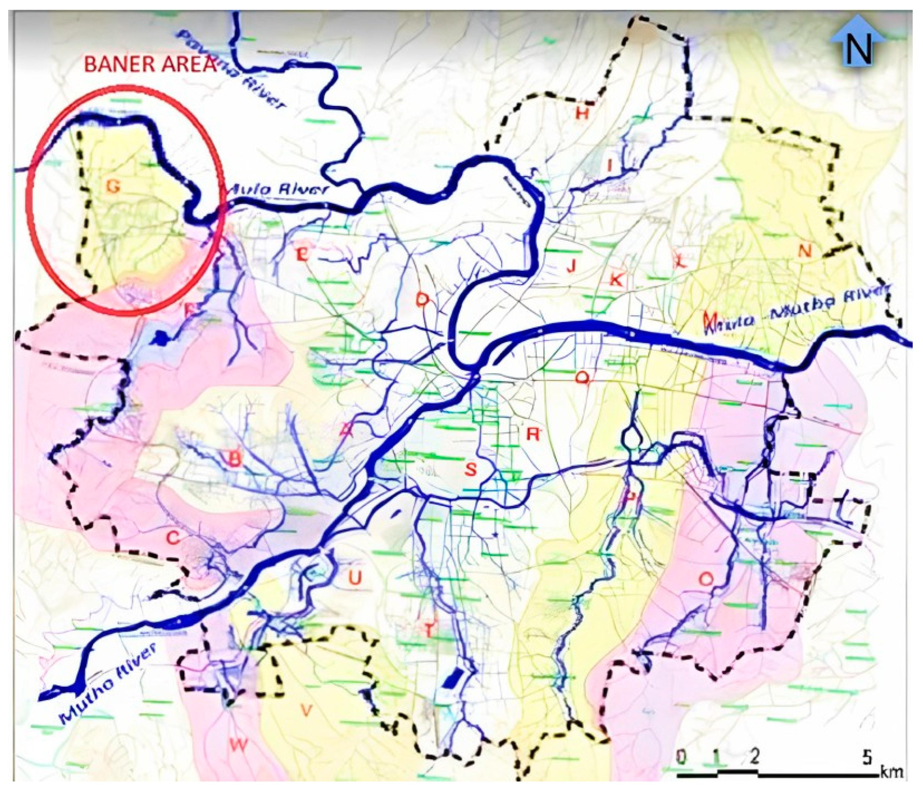
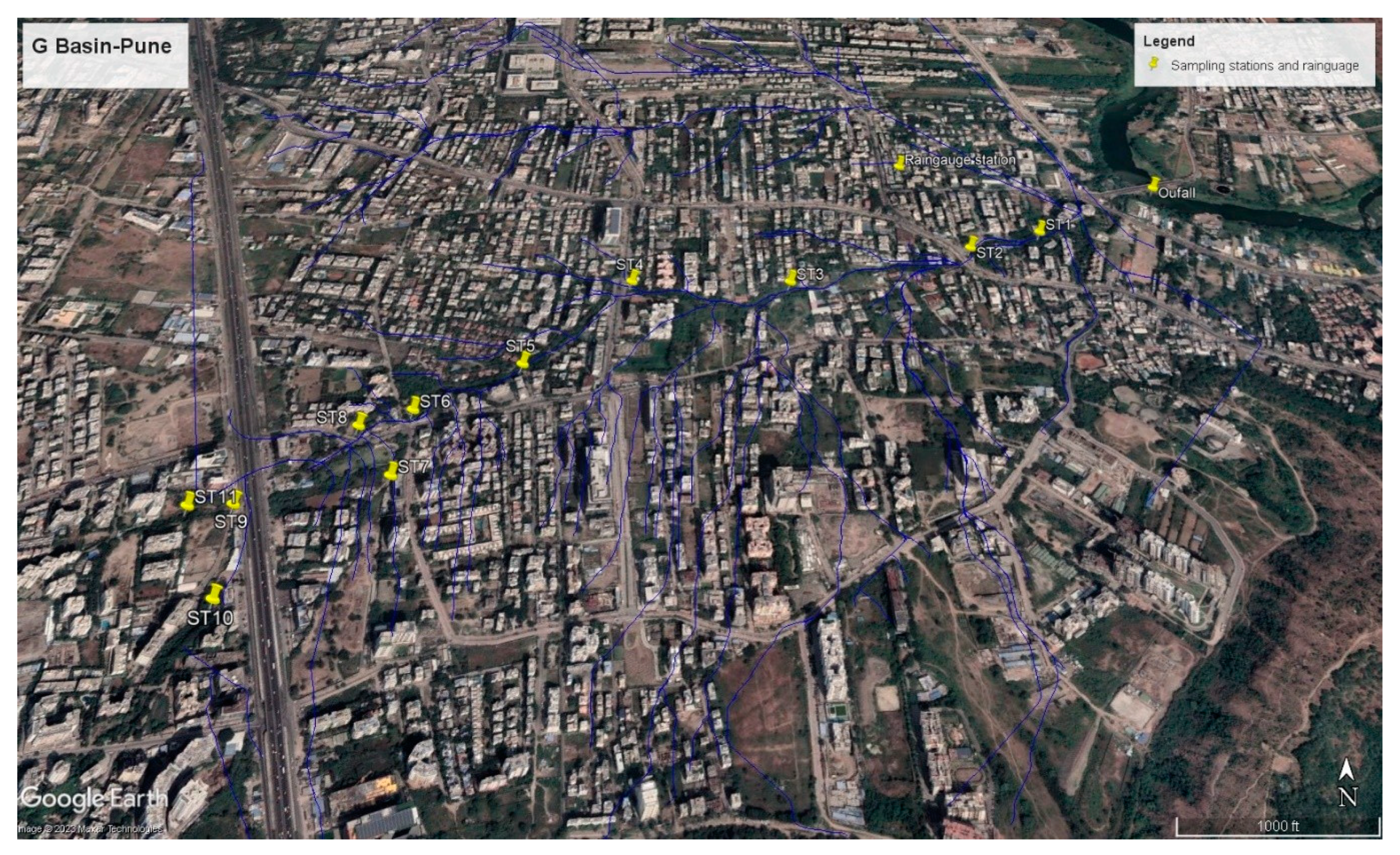
2.1. Overview of the Study Area

Pune City is one of the top ten largest cities in India, with a current estimated population of 4,307,000 [25]. It is one of the rapidly sprawling cities in western Maharashtra. It is well known as a social, commercial, industrial, and educational city, which lies between the latitude 18◦52′04″ and longitude 73◦86′00″. The city experiences tropical monsoons and encounters significant seasonal variations in temperature and rainfall conditions [26]. Rainfall is unevenly distributed within the district due to geographical conditions. During the summer, the southwest monsoon winds bring most of the rain, accounting for approximately 87% of total rainfall. The city’s annual rainfall, which is estimated to be 722 mm, falls between June to September, with July being the wettest month of the year. The city is in a hot, semi-arid region that borders a tropical, wet, and dry climate with an average temperature ranging from 19 °C (66 °F) to 33 °C (91 °F). Mula, Mutha and Mula-Mutha are three rivers that flow through the Pune Municipal Corporation area [26]. The area of Pune is split up into 23 basins, named A to W, as shown in the map in Figure 1. Each of these basins has a network of one or more naturally occurring streams that transport the stormwater into the Mula and Mutha rivers. The slopes of these networks are generally sufficient to carry reasonable stormwater runoff. These natural streams and their tributaries serve as the main drainage routes. Out of these 23 basins, G basin as highlighted in Figure 1, is a peri-urban area located on expanded peripheral boundaries of the city. G basin is a mix of land uses which includes residential, commercial, developing, and urban-rural areas.

The world urbanization prospects point out that the Pune urban clusters will have a population of 8.1 million by 2030 [27]. The urbanization rates inflate significantly, laying acute pressure on the already stretched infrastructure. This unplanned and uncontrolled expansion typically consists of randomly placed different land uses such as residential, commercial, agricultural, industrial, recreational and urban poor localities [28]. This gives rise to a mixed urban fabric with loads of pollution. Urbanization has compounded the impervious areas by around 70%, as in Figure 2 and discussed in Section 3.1 below, leaving behind very small space for green covers or sustainable stormwater drainage services. This surge in the impervious area has also raised the runoff to an enormous magnitude [29]. Rapid urbanization has substantially altered the nature of a city’s drainage patterns over time [29].

Over the period paved areas have significantly increased while the open pervious spaces disappeared. The increase in land demand, rapid urbanization, encroachment, and expansion of concrete roads have adversely affected the current natural streams, reducing their widths in several places. The urban growth along the streams has not been planned and executed scientifically. Due to this, new areas have emerged that are vulnerable to flooding even during periods of moderate rainfall [30]. This is particularly true for these newly included fringe areas in Pune Municipal Corporation. Before they entered the boundaries of the Corporation, these areas had a rural character with no control over developmental activities. The uncontrolled development of “urban poor localities” generally happened near these nallas (the naturally occurring open streams). The drainage paths have become susceptible to the build-up of various kinds of solid waste, and wastewater. For this reason, the carrying capacity has decreased, the silt load has increased and maintenance has become more challenging [28]. The natural drains cannot remove this amount of stormwater from the city’s vastly expanded settlements without the aid of an engineered stormwater system. Pune Municipal Corporation is putting efforts to line and widen these drains wherever possible to accommodate this growing volume, although the ground reality is alarming [31]. Therefore, there is a need to analyze and model the pollutants entering the natural water bodies.

In the present study, considering the mixed land use nature, the focus is on the open channel/stream/nallas where all such stormwater drains open up along with the surface runoff due to its natural slopes turning up into these natural streams. There are four main streams/natural drains flowing through the selected G basin. Out of these four streams, the longest stream (of length nearly about 4 km) located in the central part of G Basin was selected, which ultimately meets the Mula river. For the selection of sampling stations, a site survey was conducted. This site survey was done with the help of a drainage map provided by the Pune Municipal Corporation. During the survey, a total of eleven sampling stations were identified. The sampling stations were selected at the points where several small open streams or constructed stormwater drains were joining this selected stream. The sampling stations were numbered from the peripheral region towards the river from 11 to 1, respectively. The outfall sampling point, where this mainstream meets the Mula river, was also designated as shown in Figure 3.

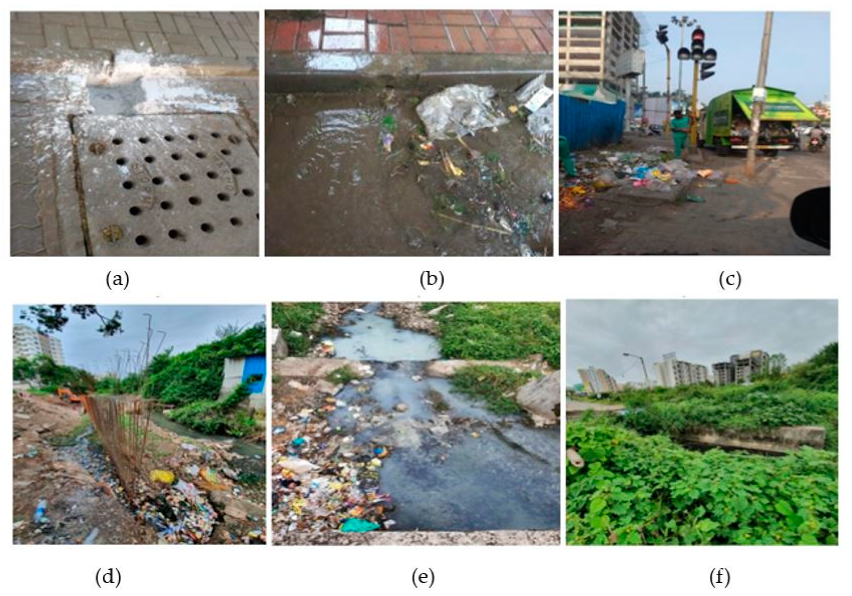
2.2. Field and Laboratory Data Collection

Manual grab sampling was carried out twice, during the rainfall and after the rainfall, at eleven sampling locations in the natural drain in an urbanized area, along with the outfall location. The samples were collected for twenty-two storm events, during the monsoon season over four years from 2018–2021. A rain logger with a data acquisition system was installed in the G basin to acquire daily precipitation data for all the twenty-two storm events. The depth and velocity were measured at all the stations, except station numbers 3,6 and 10, to ensure the continuity of the flow in the stream. These stations were inaccessible to take up the readings with depth and velocity meters. The samples were obtained in containers that had been cleaned beforehand with 10% HNO3, rinsed with tap water and distilled water, completely dried, and then sealed in the lab. The collected samples were brought to the Environmental Engineering Laboratory of Symbiosis International University. All standard sampling procedures and sampling protocols were followed during sampling using the procedures specified in the “Caltrans Stormwater Monitoring Protocol Guidance Manual” [32]. The quality assurance and quality control procedure include the suggested practices for sampling, preservation, storage, transport, laboratory testing, field blanks and laboratory blanks. Water samples were analyzed for water quality parameters, including pH, Conductivity, Turbidity, Total solids (TS), Total Suspended Solids (TSS), Total Dissolved Solids (TDS), Bio-chemical Oxygen Demand (BOD₅), Chemical Oxygen Demand (COD), Dissolved Oxygen (DO), Phosphate, Ammonia and Nitrate.

2.3. Data Pre-Processing and Analysis Techniques

Univariate statistical analysis was performed on data collected from twenty-two storm events. The missing values were determined by the predictive mean method and outliers were removed using the box detection technique. The trend analysis of spatial variation of pollutants was carried out from the farthest point towards the outfall. Furthermore, to understand the behavioral pattern, the water quality index (WQI) was calculated at all the station points [33,34]. The water quality index has been determined utilizing the standard method of drinking water quality. The calculated values were compared to the BIS standard and recommendations. The “weighted arithmetic index method” by Brown et al. 1970 [35] as shown in the following equations is used.

$$W_i=\frac{W_i}{{{\displaystyle \sum }}_{i=1}^{n}Wi}$$

(1)

where, W_i = the relative weight,

W_i = the weight of each parameter, and

n = the number of parameters

$$q_i=\left(\frac{C_i}{S_i}\right)\times 100$$

(2)

where, q_i = the quality rating,

c_i = the concentration of each parameter in each water sample in mg/L, and

s_i = the Indian drinking water standard for each parameter in mg/L, according to the guidelines of the ISI7 10500, 2012 [36].

SI_i = W_iq_i

(3)

$$\mathrm{WQI}={{\displaystyle \sum }}_{i=1}^{n}SIi$$

(4)

For computing the WQI,

SI_i= the sub-index of ith parameter.

q_i = the rating based on the concentration of ith parameter and

n = the number of parameters.

The WQI values are classified into five levels of water quality, corresponding grade and probable use as given in

Table 1. Water Quality Index, Status, Grade and probable usage [34,35].

Levels of WQI Values	Status of Water Quality	Grade	Probable Usage
0–25	Excellent	A	Drinking, Irrigation and
			Industrial
26–50	Good	B	Domestic, irrigation and
			Industrial
51–75	Poor	C	Irrigation and Industrial
76–100	Very poor	D	Irrigation
>100	Unsuitable for drinking and	E	Restricted use for
	fish culture		Irrigation

below [34,35]. For Calculating WQI, six parameters, namely, pH, Conductivity, Turbidity, BOD, TDS and DO were considered.

Principal component analysis (PCA) was conducted to find out the most influential pollutant parameters. PCA rationalises a set of raw data into a few principal components that retain the most variance within the original data. RStudio software (version 1.1.383) was used for undertaking the multivariate data analysis methods [37].

In the present study, multivariate linear regression analysis was carried out considering the stormwater quality parameter as the dependent variable, and “Rainfall” and “Antecedent Dry days (ADD)” as the independent variables.

Several non-linear methods are available for regression such as “artificial neural networks, kernel discriminant analysis, kernel partial least squares, and support vector machines” [38,39,40]. Support vector machine (SVM) is a prominent model that demonstrates an advanced form of machine learning and is well-recognized for its capability to augment regression and classification [41,42]. N. Sapankevych reviewed that “Using kernel techniques as part of a time series prediction results in a more accurate estimation of the data, even when the data series is nonlinear, non-stationary, and not characterized” [43]. SVM has the capacity to generalize due to the implementation of structural risk minimization for objective functions [44].

Support Vector Regression initially considers a basic function:

{h_m(x)}, m = 1, 2,..., M

(5)

$$f(x)={\displaystyle \sum _{m=1}^M{\beta }_m{h}_m(x)+{\beta }_0}$$

(6)

M = the number of independent variables.

To evaluate β and β₀, minimize the:

$$H(\beta ,{\beta }_0)={\displaystyle \sum _{i=1}^{N}V(y_i-f(x_i))+\frac{\lambda }{2}}{\displaystyle \sum {\beta }_m^2}$$

(7)

The solution for

$$\widehat{f(x)}={\displaystyle \sum _{m=1}^M\widehat{{\beta }_m}{h}_m(x)+\widehat{{\beta }_0}}$$

(8)

has the form

$$\widehat{f(x)}={\displaystyle \sum _{i=1}^N\widehat{{\alpha }_i}}K(x,xi)$$

(9)

where,

$$K(x,x_i)={\displaystyle \sum _{m=1}^M{h}_m(x)h_m(x_i)}$$

(10)

$$\hat{\alpha }={(H{H}^t+\lambda I)}^{-1}f(x)$$

(11)

Considering the β₀ to be consumed in the kernel function. The N × N matrix HH^t comprises inner products between pairs of observations i, i^j; i.e., the calculation of an inner product kernel {HH^t}_{i, i}^j = K (x_i, x_i^j) and I is the Identity matrix

‘W’ Coefficients that can be extracted are:

$$w={\displaystyle \sum _i{\alpha }_i{x}_i}$$

(12)

where,

i = position of the observation.

To implement Support Vector Regression on the data, RStudio software was used. In RStudio, Radial Basis Kernel Function (RBF) was found to be best suited. The Kernel Function other than RBF also gives a similar Normalized Root Mean Square Error, hence, RBF was used as a kernel function since it is provided in the RStudio Software by default.

For all the parameters radial basis kernel function was used.

$$K(x,x_i)=\exp (-\gamma ||x-x_i|{|}^2)$$

(13)

In SVM, using an RBF kernel, the data sets were tuned by the two hyperparameters C and gamma (γ). C hyperparameter contains cost and epsilon(e) parameters and it lies (0, ∞). ‘C’ value closer to zero suggests less penalty for any misfit of training data and in return reduces the training accuracy. The Gamma (γ) parameter of RBF controls the distance of the influence of a single training point. Normalized Root Mean Square Error, Coefficient of determination (R²) and the ratio of performance to the interquartile range (RPIQ) [45] was used to evaluate the predictive performance of a model, by Equations (13)–(15).

Normalized Root Mean Square Error (NRMSE) = RMSE/Mean of an observed dependent variable

(14)

R² = 1 − (sum squared regression (SSR)/total sum of squares (SST))

(15)

RPIQ = (Q3 − Q1)/RMSE

(16)

In general, having a large R² and small NRMSE means that the prediction is good. Furthermore, having larger RPIQ values means that the model predicts well.

3. Results and Discussion

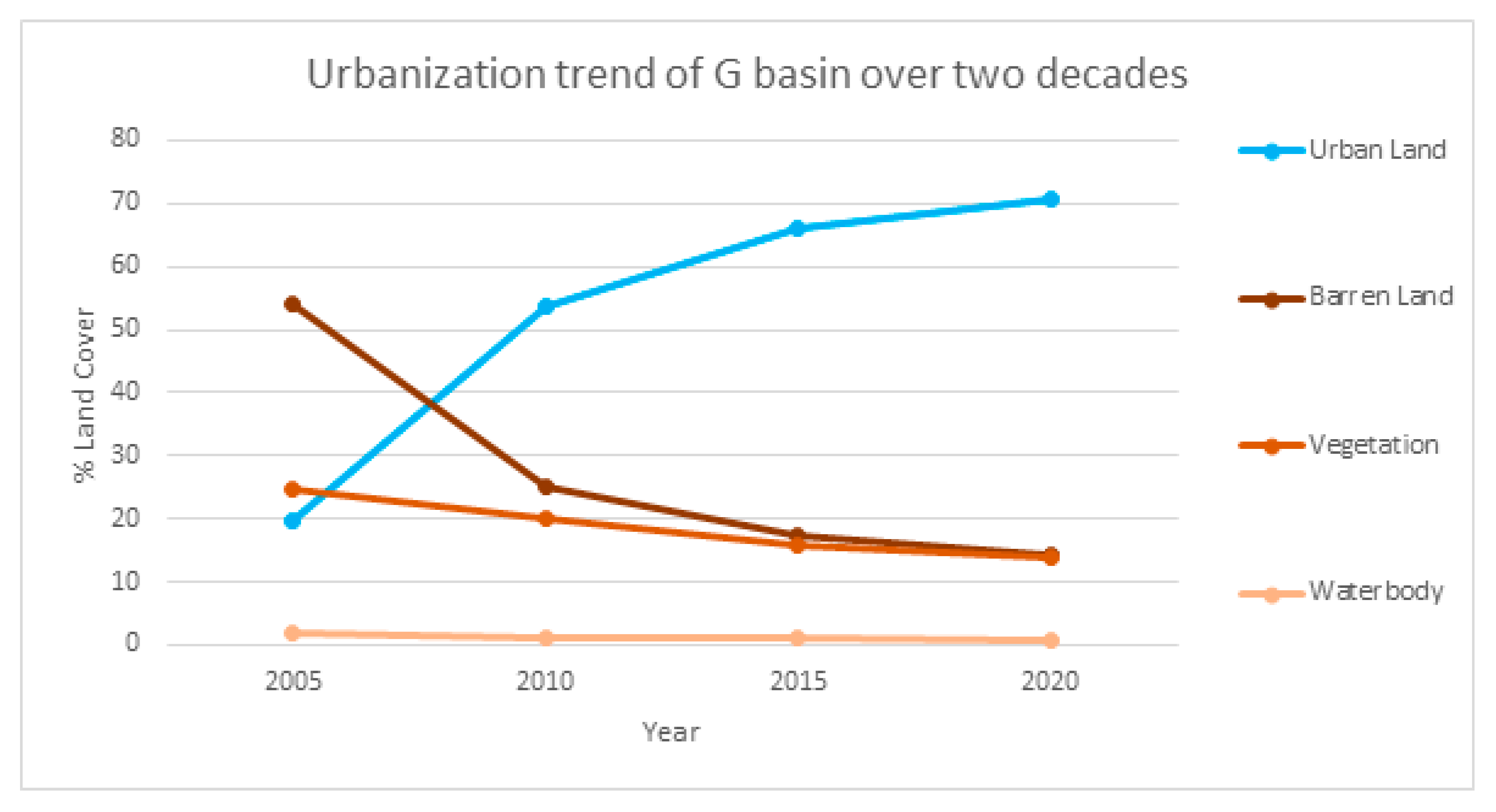
3.1. Urbanization Trend of G-Basin over Two Decades

The trend of change in the land covers of the G basin over the past two decades was studied. Landsat satellite imagery of the year 2005, 2010, 2015 and 2020 was classified by the Maximum likelihood classification method using ArcMap 10.6.1 to obtain the land use maps. In this study, the image was classified into Urban areas (mixed development), Vegetation cover, Barren land, and waterbody, as shown in Figure 2. The graph in Figure 4 shows the patterns of change in land cover type over twenty years from 2005 to 2020. The graph shows a burgeoning increase in urban land between the years 2005 to 2020, reducing barren land to almost half of its area, and indicating the onset of urban sprawl in the G-basin. Urban areas increased up to 70% in the year 2020 with a reduction of 10% in vegetation cover and up to 40% reduction in barren land. The urbanization trend also portrays a marginal decrease in water bodies; for this there are many possible reasons, including human encroachment and climate change.

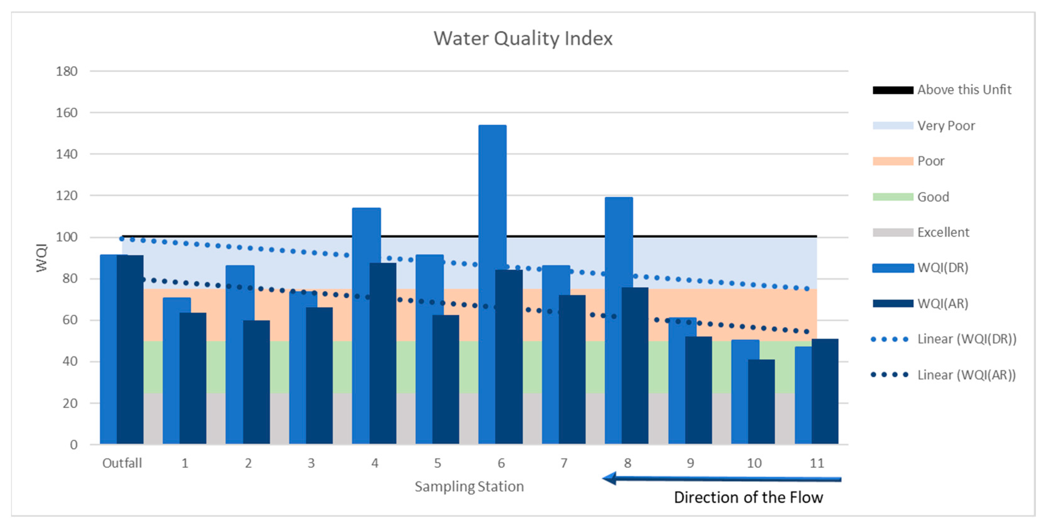
3.2. Stormwater Quality Analysis of Urban Surface Runoff

As discussed in Section 2.3, the predictive mean method was used to determine 9% of the missing values. It was mainly because of the inaccessibility of the stream site due to the large growth of weeds as shown in Figure 5f. Table 1 provides the mean concentration and standard deviation (SD) of quality parameters for various station points on the stream. The Bureau of Indian Standards for categorizing surface water sources describe that the quality of water is below class E [46,47]. The parameters were deteriorated beyond class E and appear like sewage or industrial effluents. Therefore, this stormwater certainly demands treatment before discharge.

For further analysis, the spatial behavioral trends were observed station-wise from the farthest station number 11 towards the outfall. The data were also analyzed to compare pollutant concentrations during rainfall and after rainfall at each station. The pollutant concentration of turbidity, TSS, TDS and COD show an increasing trend from peripheral stations towards the discharging point at the outfall. It is also observed that the pollution concentration of TDS, TSS, DO, BOD, COD and phosphates were higher for the samples collected during the rainfall. The higher concentrations of BOD and COD may be organic in nature possibly because of the erosion of roadsides due to surface runoff. The presence of animal excreta, human faeces due to open defecation and leakage in sewage drainage lines were also identified as additional sources. There were no curbs on the roads in several places. The channeling at most of the places was also missing. Thus, the grass cover, loose soil, or dust present on the roadside was picked up by the surface runoff. The main reason for an increase in phosphate concentration is likely to be originated from decomposed plant materials such as leaves, grass clippings and eroded soil [8].

The variation in the spatial distribution of impervious regions significantly affects pollution concentrations [6,48]. The time and velocity of travel of surface runoff towards these naturally occurring open channels certainly affect the pollution concentrations at these sampling locations. The pollution concentration ranges of ammonia and nitrate were observed to be more for the samples collected after the rainfall. The nitrogenous concentrations can be attributed to the leaching of fertilizers from lawns, parks and agricultural lands present in the study area located slightly away from the open channel [8].

The standard deviation is observed to be higher for solids parameters, turbidity, BOD, COD and phosphate, which indicates huge variations in stormwater quality. This makes urban stormwater quality control more challenging to understand. The variations in the quality parameters at all the stations are attributed to the mixed land usage, the haphazard distribution of impervious and pervious areas and the lack of appropriate management practices with a primary focus on quality. These variations can also be justified by field observations such as improper solid waste management practices near the roadside drains as well as in the streams. The variation in stormwater quality can also be attributed to the throwing of paints, chemicals and other liquid wastes in these stormwater drains/open streams, and the encroachment of these streams by carrying out construction activities. The images of these field observations of the study area are shown in Figure 5.

The WQI values were calculated as shown in Equation (1) and, as shown in Figure 6, ranged from 46.9 to 153.9 for the samples collected during rainfall, and from 41.20 to 87.70 for samples collected after rainfall. It is noted that the values of the physicochemical parameters increased substantially for samples taken during the storm event than those taken after the storm event. This trend was observed at all the sampling stations. The WQI values during the storm event were greater than the samples collected after the storm event. This also reflects the first-flush effect during the storm event, which reduces after the rainfall. In both cases, the WQI values exhibited an increasing trend towards the outfall. Moreover, the majority of the WQI parameters are of poor to very poor water quality levels, as referred to in

Table 2. Mean values and standard deviation of the parameters analyzed.

	pH	CONDUCTIVITY	TURBIDITY	TDS	TSS	TS	DO	BOD	COD	Phosphate	Ammonia	Nitrate
Unit	mg/L	µs/m	NTU	mg/L	mg/L	mg/L	mg/L	mg/L	mg/L	mg/L	mg/L	mg/L
Mean	7.883	0.795	37.4	514.8	927	1448	2.9	110	513.4	0.74	0.386	0.232
SD	0.067	0.157	10.2	57.2	185	180	0.7	22.9	76.5	1.63	0.103	0.085

. This analysis strongly justifies the need for a specific degree of source control treatment measures before the stormwater merges into the Mula river.

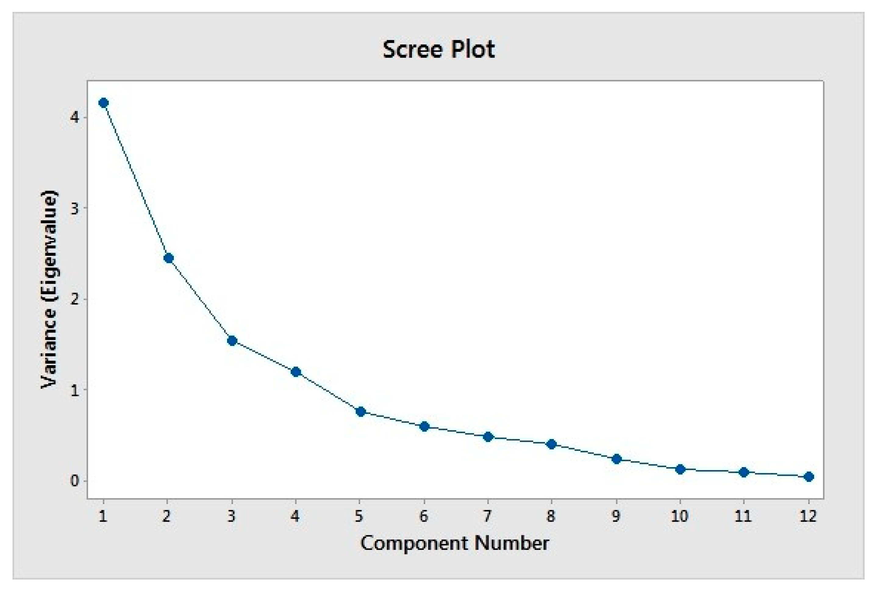
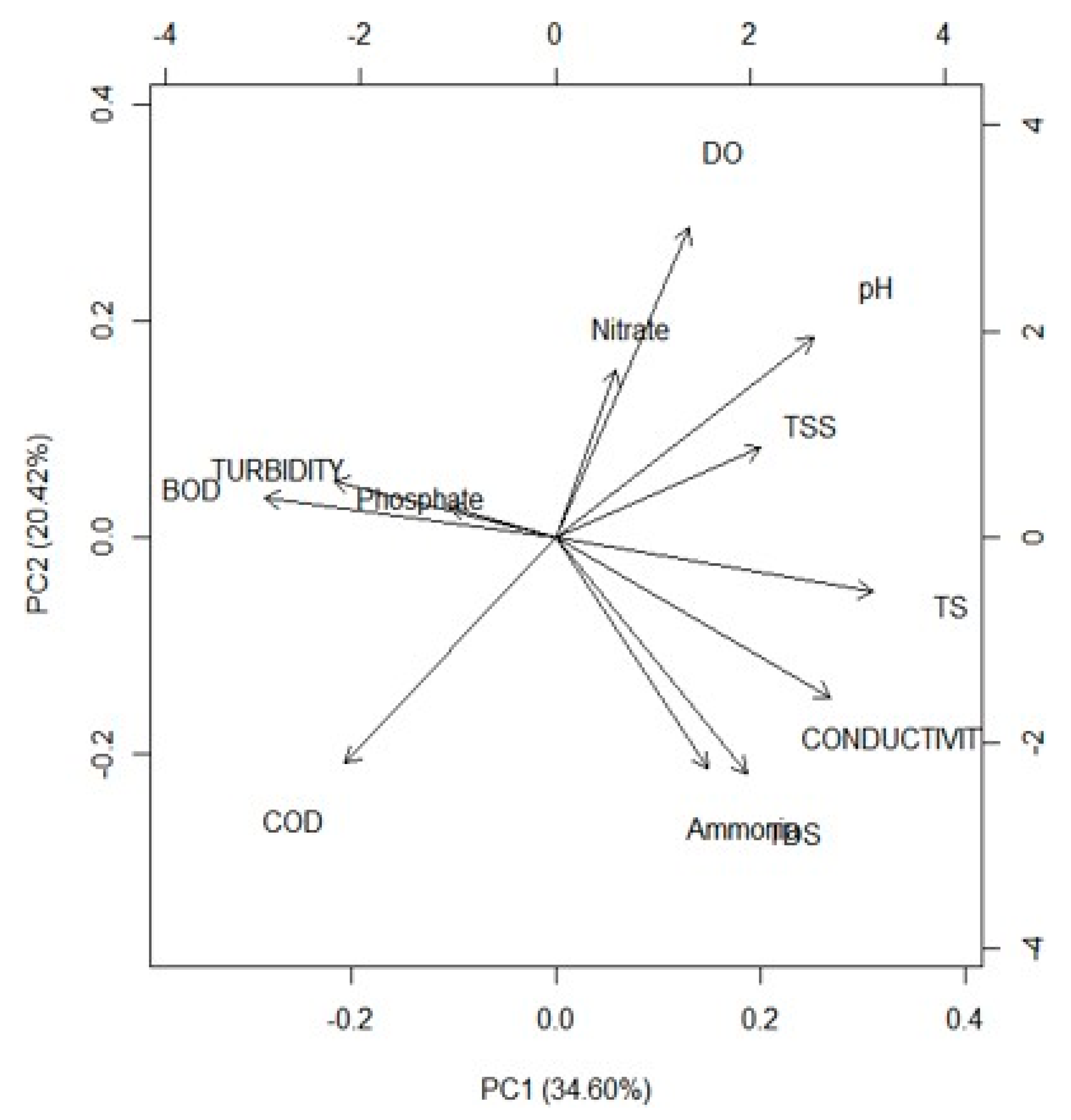
3.3. Significant Stormwater Quality Parameters

There were considerable ambiguities in the attempts to formulate the process of pollution generation, its transmission and dispersal. This implies that the urban form has an impact on the properties of primary stormwater pollutants, which suggests that the effectiveness of structural measures cannot be universal but needs to be addressed locally [8]. To explore this association among different pollutant parameters for mixed land use in the current study of the peri-urban area, Principal Component Analysis (PCA) was used, as discussed in Section 2.3.

Out of the twelve parameters, the components with the highest total variance were considered the most significant. The number of significant principal components was determined using Kaiser’s criteria. The scree plot of components, as shown in Figure 7, also exhibited that only four components, having eigenvalues greater than one, were retained. These components reported for 77.7% of the total variance, out of which the first component (PC1) and the second component (PC2) accounted for 34.60% and 20.42% of the total variance, respectively. They also strongly exhibited a positive relationship with TS and dissolved oxygen, respectively. Whereas the third component (PC3) accounted for 13% of the total variance and exhibited a positive association of TSS, Phosphate, and Nitrate. However, the fourth component (PC4) accounted for only 9% of the total variance and showed a positive relationship with turbidity. Thus, the most significant stormwater quality parameters are TS, DO, TSS, Phosphate, Nitrate and Turbidity. Biplots were used to determine the type of relationship among the parameters present. Each vector represents individual parameters. The angle between the vectors is inversely proportional to the correlation. The closer the vectors are to one another more the correlation. Vectors are negatively correlated when they lie opposite each other. Vectors which are perpendicular to each other are said to be uncorrelated.

From the biplot in Figure 8, between the first two components, which accounts for 55% of the total variance, a positive correlation was observed between Ammonia and TDS. From this, it can be concluded that most of these nutrients were in the dissolved state. A positive correlation was also observed between Phosphate, Turbidity and BOD, which implies that these types of nutrients and organic load are particle bound. Similarly, it was observed from a biplot, as shown in Figure 9, for PC1 and PC3, that DO, TDS and pH were strongly correlated. The positive correlation among turbidity, COD and BOD highlights that the pollutant load is particle bound, as together they negatively correlated with TS. Stormwater management begins at the point when the raindrops strike the ground surfaces. Firstly, non-structural measures include source control, where practices can be incorporated which remove the pollutants before contact with rainfall. One of them is regular sweeping of roads, cleaning of open streams before monsoon, washing of the roads, maintenance of the stormwater drainage facilities, etc. The second part, that is the structural measures, includes the adoption of one or more multiple source control measures/low impact development practices, which are reducing the volumes and pollution from the stormwater. The analysis of significant stormwater quality parameters, the inter-relation and their nature will help the decision makers to develop the strategies for source control as well as to prevent the build-up of these pollutants. Furthermore, it is vital to understand if any correlation exists between these stormwater quality parameters and rainfall characteristics further discussed in the next section.

3.4. Relationship of Stormwater Quality Parameters with Rainfall Characteristics

From the literature, many studies were undertaken to understand the influence of rainfall characteristics on pollutant concentrations in stormwater. Yongwei Gong and Xiaoying Liang [49] analyzed the temporal distribution of rainfall, rainfall depth and rainfall duration under different dry days to understand the dual effect of rainfall characteristics and surface flooding on TSS at the outfall of the catchment. Arora et al. (2013) took up the regression analysis of varied sub-watersheds [8]. Rainfall and antecedent dry days were the two independent variables that were subjected to linear regression analysis with pollution concentrations as BOD, COD, TSS, TDS, TKN, TP, oil and grease, total and faecal coliforms and heavy metals acting as the dependent variables [8]. It was observed that the coefficient of determination for each model was not significantly higher than 50% for any of the parameters. This inference suggests that the behaviour of the data was not linear. The previous studies have considered sampling at a single point at upland surfaces, where the liner models worked aptly. In this study, the in-stream behaviour of pollutants for various sampling points for sub-watersheds of varied mixed land use may be the reason attributed to the observed non-linearity.

For this non-linear regression, a machine learning algorithm ‘Support Vector Regression (SVR)’ was considered, as discussed in Section 2.3. This machine learning algorithm works fine for a small set of observations, unlike other machine learning regression algorithms. One of the key features of Support Vector Regression (SVR) is that it aims to minimize the generalized error bound, rather than the observed training error to accomplish generalized performance. This generalization error bound is the blend of the training error and a regularization term that monitors the complexity of the hypothesis space. In classical support vector regression, it is challenging to define the proper value for the parameter ε in advance. Fortunately, a new algorithm—“ν support vector regression” (ν-SVR)—partially solves this issue, where, “ε itself is a variable in the optimization process”, and is regulated by another new parameter “ν ∈ (0, 1)”. “ν is the upper bound on the fraction of error points or the lower bound on the fraction of points inside the ε-insensitive tube. Thus, a right ε can be automatically found by choosing the appropriate ν, which adapts the accuracy level to the data at hand. This makes ν a more suitable parameter than the one used in ε-SVR”.

After fitting the SVR model for this parameter, the parameters were tuned to better optimize the kernel function. The complete data for each parameter was divided into four different combinations of training and testing sizes, viz. 70–30%, 80–20%, 90–10% and 95–5%, as input. For each parameter, the combination depicting the least difference in training and testing error was the best fit, as shown in

Table 3. Training and testing best-fit size displaying the least difference.

Parameters	Training Size (%)	Testing Size (%)	Training Error	Testing Error	Difference (Training and Testing)
TUR-	70	30	30.47	45.88	15.41
BIDITY
TS	90	10	107.47	162.61	55.14
TSS	80	20	91.62	166.37	74.75
DO	80	20	0.27	1.42	1.15
Phos-	95	5	0.008	0.011	0.003
phate
Nitrate	90	10	0.01	0.014	0.004

. Hence, this size of training and testing data will give the most accurate prediction.

Table 4. Results of the Support Vector Regression Models.

Parameters	Co-Efficient for Rainfall	Co-Efficient for ADD	Bias (Constant)	NRMSE	R2	RPIQ
TURBID-	−0.17702	0.767276	0.24	0.85	0.39	0.79
ITY
TS	−3.08976	3.140374	−0.01	0.17	0.82	2.91
TSS	−2.70495	3.053751	0.03	0.3	0.75	2.23
DO	0.63459	1.086196	0.28	0.44	0.79	1.93
Phos-	−1.61594	2.415755	0.2	0.02	0.67	1.62
phate
Nitrate	0.853082	−0.63948	0.08	0.03	0.72	1.48

shows the results of the support vector regression models, where the coefficients of rainfall and antecedent dry days were derived. The coefficients shown in Table 4 are in the form given in Equation (16).

The coefficients suggest that a unit increase/decrease in the value of Rainfall (mm) and ADD (days) results in a weighted (α_i, for i^th observation) increase/decrease in the value of the stormwater quality parameter. Non-linear SVR models confirmed that both antecedent dry days and rainfall are correlated with stormwater quality. Table 4 depicts NRMSE, R² and RPIQ values to evaluate the accuracy of the models. The SVR model depicted the best performance for parameter TS with NRMSE (0.17), R² (0.82) and RPIQ (2.91). Except for turbidity NRMSE (0.85), R² (0.39) and RPIQ (0.79), all the other parameters have a good fit for the SVM model of regression for the radial basis function. This suggests turbidity also be dependent on other rainfall characteristics, apart from the rainfall and ADD.

Knowing the two variables of ADD and Rainfall, this modelling was performed to predict the concentration levels of the pollutant parameters that fit well within the model. It is vital to first assess runoff characteristics and meticulously analyse the actual situation with respect to rainfall and catchment characteristics before initiating structural control strategies. During storm events, hydraulic and physical processes remove larger solids and associated pollutants, while biological and chemical processes treat finer solids and dissolved pollutants [50]. These holistic solutions depend on many factors, including the availability of appropriate space in the peri-urban area, physical site conditions, as well as regulatory requirements. This study will aid to design a treatment train approach of source control measures with the purpose to control the pollutants at the source and further a stormwater treatment facility to minimize the volume and pollution loads entering the open stream.

4. Conclusions

It is observed from the experimental investigations that the stormwater quality parameters have deteriorated below class E, which is equivalent to sewage or industrial effluents. The values of the physicochemical parameters significantly increased for samples taken during the storm event. This pattern was observed across all sampling stations. Water Quality Index (WQI) values for the samples collected during the storm event were higher than those for samples collected after the storm event. The WQI values show an increasing trend from the peripheral region towards the outfall location in the river. Most of the WQI values fall in poor to very poor water quality levels, with few of them above the unfit mark.

Principal component analysis (PCA) identified TS, DO, TSS, Phosphate, Nitrate and Turbidity as the most significant stormwater quality parameters. The PCA biplots showed a positive correlation among various parameters. The SVR model with radial basis kernel function (RBF) is developed to understand the non-linear complex behaviour of rainfall characteristics with these stormwater pollutant parameters. The normalized root mean square error determines the accuracy of each model. The unit increase or decrease in the coefficients of rainfall characteristics displays the weighted deviation in the values of pollutant parameters.

This study demonstrates that assessing the stormwater characteristics and meticulous consideration of all the existing conditions is crucial before embarking on expensive source control strategies. Location-specific analysis can more accurately handle pollutant reduction efforts to achieve sustainable solutions for such scenarios in developing cities. Overall, given the cost of treatment in developing countries, source control strategies should be the main focus of management practices, rather than stormwater runoff treatment. An integrated land use planning and design strategy to mitigate land use planning impacts on the environment is increasingly being promoted as an impactful method of reducing runoff and pollutant loadings into streams. The conclusions drawn can provide effective information to decision-makers to employ an appropriate treatment train approach of varied source control measures to be proposed to treat and mitigate runoff in an open stream rather than an end pipe approach. This will holistically serve the stakeholder’s objectives to manage stormwater efficiently. The research work can be further augmented by adopting selecting a multi-criteria decision-making tool to adopt the best SCM and its multiple potential combinations.

References

1. United Nations. “Peace, Dignity and Equality on a Healthy Planet,” [Online]. 2022. Available online: https://www.un.org/en/global-issues/population (accessed on 3 March 2023).
2. Boretti, A.; Rosa, L. Reassessing the projections of the World Water Development Report. Npj Clean Water 2019, 2, 15. [Google Scholar] [CrossRef] [Green Version]
3. The United Nations World Water Development Report 2021: Facts and Figures. Valuing Water; UNESCO: Paris, France, 2021; pp. 1–12.
4. Lin, L.; Yang, H.; Xu, X. Effects of Water Pollution on Human Health and Disease Heterogeneity: A Review. Front. Environ. Sci. 2022, 10, 1–16. [Google Scholar] [CrossRef]
5. Bolliger, J.; Silbernagel, J. Contribution of connectivity assessments to green infrastructure (GI). ISPRS Int. J. Geo-Inf. 2020, 9, 1–17. [Google Scholar] [CrossRef] [Green Version]
6. Liu, A.; Goonetilleke, A.; Egodawatta, P. Role of Rainfall and Catchment Characteristics on Urban Stormwater Quality. In SpringerBriefs in Water Science and Technology; Springer: Berlin/Heidelberg, Germany, 2015. [Google Scholar] [CrossRef] [Green Version]
7. Marsalek, J.; Watt, W.E.; Anderson, B.C. Trace metal levels in sediments deposited in urban stormwater management facilities. Water Sci. Technol. 2006, 53, 175–183. [Google Scholar] [CrossRef] [PubMed] [Green Version]
8. Arora, A.S.; Reddy, A.S. Multivariate analysis for assessing the quality of stormwater from different Urban surfaces of the Patiala city. Urban Water J. 2013, 10, 422–433. [Google Scholar] [CrossRef]
9. Gogate, N.G.; Rawal, P.M. Identifying objectives for sustainable stormwater management in urban Indian perspective: A case study. Int. J. Environ. Eng. 2015, 7, 143–162. [Google Scholar] [CrossRef]
10. US EPA. Protecting Water Quality from Urban Runoff; US EPA: Washington, DC, USA, 2003. Available online: www.epa.gov/nps (accessed on 15 January 2023).
11. Lee, F.; Jones-Lee, A. Urban Stormwater Runoff Water Quality Issues. Water Encyclopedia: Surface and Agricultural Water; Wiley: Hoboken, NJ, USA, 2005; pp. 432–437. [Google Scholar]
12. Müller, A.; Österlund, H.; Marsalek, J.; Viklander, M. The pollution conveyed by urban runoff: A review of sources. Sci. Total Environ. 2020, 709, 136125. [Google Scholar] [CrossRef]
13. United Nations World Water Assessment Programme, UN-Water. The United Nations World Water Development Report 2018: Nature-Based Solutions for Water; UNESCO: Paris, France, 2018. [Google Scholar]
14. Goonetilleke, A.; Thomas, E.; Ginn, S.; Gilbert, D. Understanding the role of land use in urban stormwater quality management. J. Environ. Manag. 2005, 74, 31–42. [Google Scholar] [CrossRef] [Green Version]
15. Huang, J. Characterization of surface runoff from a subtropics urban catchment. J. Environ. Sci. 2007, 19, 148–152. [Google Scholar] [CrossRef]
16. Imteaz, M.A.; Hossain, I.; Hossain, M.I. Estimation of build-up and wash-off models parameters for an east-australian catchment. Int. J. Water 2014, 8, 48–62. [Google Scholar] [CrossRef]
17. Kim, L.H.; Zoh, K.D.; Jeong, S.; Kayhanian, M.; Stenstrom, M.K. Estimating Pollutant Mass Accumulation on Highways during Dry Periods. J. Environ. Eng. 2006, 132, 985–993. [Google Scholar] [CrossRef]
18. Ahyerre, M.; Chebbo, G.; Tassin, B.; Gaume, E. Storm water quality modelling, an ambitious objective? Water Sci. Technol. 1998, 37, 205–213. [Google Scholar] [CrossRef]
19. Rosa, L.D.; Pappalardo, V. Planning for spatial equity—A performance-based approach for sustainable urban drainage systems. Sustain. Cities Soc. 2019, 53, 101885. [Google Scholar] [CrossRef]
20. Chapman, C.; Hall, J.W. Designing green infrastructure and sustainable drainage systems in urban development to achieve multiple ecosystem benefits. Sustain. Cities Soc. 2022, 85, 104078. [Google Scholar] [CrossRef]
21. Gimenez-Maranges, M.; Pappalardo, V.; Rosa, D.; Breuste, J.; Hof, A. The transition to adaptive storm-water management: Learning from existing experiences in Italy and Southern France. Sustain. Cities Soc. 2020, 55, 102061. [Google Scholar] [CrossRef]
22. Trifi, M. Machine learning-based prediction of toxic metals concentration in an acid mine drainage environment, northern Tunisia. Environ. Sci. Pollut. Res. 2022, 29, 87490–87508. [Google Scholar] [CrossRef]
23. Zhang, H. Machine learning-based source identification and spatial prediction of heavy metals in soil in a rapid urbanization area, eastern China. J. Clean. Prod. 2020, 273, 122858. [Google Scholar] [CrossRef]
24. Khoi, D.N.; Quan, N.T.; Linh, D.Q.; Nhi, P.T.T.; Thuy, N.T.D. Using Machine Learning Models for Predicting the Water Quality Index in the La Buong River, Vietnam. Water 2022, 14, 1552. [Google Scholar] [CrossRef]
25. “Population Census.” [Online]. Available online: https://www.census2011.co.in/census/city/375-pune.html (accessed on 16 February 2023).
26. “Pune Municipal Corporation.” [Online]. Available online: https://www.pmc.gov.in/en/pune-weather-0 (accessed on 16 February 2023).
27. Butsch, C.; Kumar, S.; Wagner, P.D.; Kroll, M.; Kantakumar, L.N.; Bharucha, E.; Schneider, K.; Kraas, F. Growing ‘Smart’? Urbanization Processes in the Pune Urban Agglomeration. Sustainability 2017, 9, 2335. [Google Scholar] [CrossRef] [Green Version]
28. Pune Municipal Corporation. Revised City Development for Pune-2041: Physical Infrastructure; Under JNNURUM: Maharashtra, India, 2012; pp. 96–162. [Google Scholar]
29. Gogate, N.G.; Rawal, P.M. Identification of potential stormwater recharge zones in dense urban context: A case study from Pune city. Int. J. Environ. Res. 2015, 9, 1259–1268. [Google Scholar]
30. Gogate, N.G.; Rawal, P.M. Sustainable Stormwater Management in Developing and Developed Countries: A Review. In Proceedings of the International Conference on Advances in Design and Construction of Structures, Bangalore, India, 19–20 October 2012; pp. 1–6. [Google Scholar]
31. PMC-Pune Municipal Corporation. Comprehensive Master Plan of Pune City; Pune Municipal Corporation: Pune, India, 2009. [Google Scholar]
32. State of California Department of Transportation. Caltrans Stormwater Monitoring Guidance Manual. In Environmental Analysis Stormwater Program; State of California Department of Transportation: Sacramento, CA, USA, 2020. Available online: http://www.dot.ca.gov/hq/env/stormwater/ (accessed on 25 January 2023).
33. Mohd Hafiyyan, M. Spatial Distribution of Water Quality Index in Stormwater Channel: A Case Study of Alur Ilmu, UKM Bangi Campus. Asia Pac. Environ. Occup. Health J. 2017, 3, 33–38. [Google Scholar]
34. Datta, S.; Ground, C.; Board, W.; Kushwaha, A. Weighted Arithmetic Water Quality Index Method for Ground Water Quality Determination in and around Guwahati. In Proceedings of the conference on water resources on eastern and Northe eastern states of India, Kolkata, India, June 2018. [Google Scholar]
35. Brown, R.M.; Mcclelland, N.I.; Deininger, R.A.; Tozer, R.G. A Water Quality Index—Do We Dare? Water Sew. Work. 1970, 117, 339–343. [Google Scholar]
36. Indian Standard Drinking Water Specification. Bur. Indian Stand. 2012, 10500, 1–11.
37. Hastie, T.; Tibshirani, R.; James, G.; Witten, D. The Elements of Statistical Learning; Springer series in statistics: New York, NY, USA, 2008; pp. 1–764. [Google Scholar]
38. Jadhav, M.S.; Khare, K.C.; Warke, A.S. Water Quality Prediction of Gangapur Reservoir (India) Using LS-SVM and Genetic Programming. Lakes Reserv. Res. Manag. 2015, 20, 275–284. [Google Scholar] [CrossRef]
39. Singh, K.P.; Basant, N.; Gupta, S. Support vector machines in water quality management. Anal. Chim. Acta 2011, 703, 152–162. [Google Scholar] [CrossRef]
40. Kamyab-Talesh, F.; Mousavi, S.F.; Khaledian, M.; Yousefi-Falakdehi, O.; Norouzi-Masir, M. Prediction of Water Quality Index by Support Vector Machine: A Case Study in the Sefidrud Basin. Water Resour. 2019, 46, 112–116. [Google Scholar] [CrossRef]
41. Yoon, H.; Kim, Y.; Ha, K.; Lee, S.H.; Kim, G.P. Comparative evaluation of ANN-and SVM-time series models for predicting freshwater-saltwater interface fluctuations. Water 2017, 9, 323. [Google Scholar] [CrossRef] [Green Version]
42. Niu, W.; Feng, Z.K. Evaluating the performances of several artificial intelligence methods in forecasting daily streamflow time series for sustainable water resources management. Sustain. Cities Soc. 2020, 64, 102562. [Google Scholar] [CrossRef]
43. Sapankevych, N.; Sankar, R. Time series prediction using support vector machines: A survey. IEEE Comput. Intell. Mag. 2009, 4, 24–38. [Google Scholar] [CrossRef]
44. Chou, P.H.; Wu, M.J.; Chen, K.K. Integrating support vector machine and genetic algorithm to implement dynamic wafer quality prediction system. Expert Syst. Appl. 2010, 37, 4413–4424. [Google Scholar] [CrossRef]
45. Gasmi, A.; Gomez, C.; Chehbouni, A.; Dhiba, D.; Gharous, M.E. Using PRISMA Hyperspectral Satellite Imagery and GIS Approaches for Soil Fertility Mapping (FertiMap) in Northern Morocco. Remote Sens. 2022, 14, 4080. [Google Scholar] [CrossRef]
46. ENVIS Centre. Punjab BIS (ISI) Water Quality Standards for Classifying Surface Water Sources, By Ministry of Environment, Forests & Climate Change, Govt of India BIS. BIS 2020, 2–3. [Google Scholar]
47. “Central Pollution Control Board (CPCB), Ministry of Environment Forest and Climate Change, Government of India.” [Online]. 2023. Available online: https://cpcb.nic.in/water-quality-criteria/ (accessed on 16 February 2023).
48. Wijesiri, B.; Egodawatta, P.; Mcgree, J.; Goonetilleke, A. In fl uence of uncertainty inherent to heavy metal build-up and wash- off on stormwater quality. Water Res. 2016, 91, 264–276. [Google Scholar] [CrossRef] [PubMed] [Green Version]
49. Gong, Y.; Liang, X.; Li, X.; Li, J.; Fang, X.; Song, R. Influence of rainfall characteristics on total suspended solids in urban runoff: A case study in Beijing, China. Water 2016, 8, 278. [Google Scholar] [CrossRef] [Green Version]
50. Fletcher, T.D. SUDS, LID, BMPs, WSUD and more—The evolution and application of terminology surrounding urban drainage. Urban Water J. 2015, 12, 525–542. [Google Scholar] [CrossRef]
Figure 1. Pune drainage Map-showing study area G Basin [28].
Hydrology 10 00066 g001
Figure 2. Land use classification maps over the twenty years respectively, (a) 2005; (b) 2020.
Hydrology 10 00066 g002
Figure 3. Main natural stream in Baner-showing 11 sampling locations along with an outfall location on river Mula. (Google Earth Image).
Hydrology 10 00066 g003
Figure 4. Urbanization trend of G-basin over two decades.
Hydrology 10 00066 g004
Figure 5. Study area images (a) Throwing of chemicals/paints in the stormwater drain, (b) Choking of drains due to waste on road, (c) Improper solid waste management practices, (d) Construction activity near the stormwater drain, (e) Liquid waste in the open stream, (f) Sampling station inaccessible due to weeds growth.
Hydrology 10 00066 g005
Figure 6. Water Quality Index at sampling stations.
Hydrology 10 00066 g006
Figure 7. Scree plot of components.
Hydrology 10 00066 g007
Figure 8. Biplots PC1 vs. PC2.
Hydrology 10 00066 g008
Figure 9. Biplots PC1 vs. PC3.
Hydrology 10 00066 g009