Article

Reservoir Capacity Estimation by the Gould Probability Matrix, Drought Magnitude, and Behavior Analysis Methods: A Comparative Study Using Canadian Rivers

Department of Civil Engineering, Lakehead University, Thunder Bay, ON P7B 5E1, Canada
*
Author to whom correspondence should be addressed.
Hydrology 2023, 10(2), 53; https://doi.org/10.3390/hydrology10020053
Submission received: 13 January 2023 / Revised: 8 February 2023 / Accepted: 15 February 2023 / Published: 20 February 2023
(This article belongs to the Section Statistical Hydrology)

Abstract

:
Among the various methods for estimating reservoir volumes, the Gould probability matrix (GPM) method has been touted as a powerful method for estimating reservoir volumes. The other methods in vogue are the Behavior analysis (BA) with the latest induction of the Drought magnitude (DM) method. A comparison of the above methods in terms of ease, efficiency, and relative merits from each other is currently lacking in the literature. This paper compares the above three methods with a detailed analysis of the GPM method using the monthly flows from 16 Canadian rivers at the draft ratios of 75 and 50% with the probability of failure of 2.5, 5 and 10%. The results reported in this paper indicate that fifteen zones are sufficient in the GPM method to yield the reservoir capacity for the Canadian rivers while requiring no standardization of the data, similar to the BA method. In the DM method, standardized monthly flow sequences in combination with a scaling parameter Φ yielded effective drought length, which, when multiplied by drought intensity and the average of 12 monthly standard deviations, resulted in the appropriate values of reservoir capacity. The results of this paper affirm that the GPM method offers little special merit in obtaining reservoir capacity in view of the rigor of computational efforts and uncertainty in the correction factors for significantly autocorrelated (dependent) annual flows. The DM method was found to be comparable to the BA method, though it requires standardization of the monthly flow data. The study suggests that all three methods result in comparable estimates of reservoir capacity for nearly independent annual flows with a slight edge to the Behavior analysis (BA) method.

1. Introduction

The reservoir capacity or volume (CR) can be estimated using river flows for a given draft ratio (α) and the probability of failure (PF) for supplying the water. The draft ratios are expressed as the ratio to the mean annual flow (MAF), such as 75% (0.75 µa), 50% (0.50 µa), etc., where µa is the mean of the annual flow sequences (MAF) under consideration. The flows from a river can be analyzed using annual, monthly, or weekly scales for assessing the reservoir capacity. The mean flow would turn out to be nearly the same at all scales, though the variance and autocorrelation structure would differ significantly from each other at respective scales. A majority of reservoirs across the globe are designed for α ranging from 40 to 90% [1] with an adopted α of 75% [2,3,4]. At times, reservoirs with α in the vicinity of 50% also are in existence [1,5]. The monthly scale of flows is deemed adequate in sizing the reservoirs [2,3,4]. The other important parameter associated with sizing a reservoir is the probability of failure (PF) of the reservoir to supply water to meet the demand. For pragmatic reasons, the PF values of 2.5, 5, and 10% are regarded as satisfactory [3], though theoretically, PF as low as 0% can be used to calculate the reservoir capacity. A large reservoir is not easy to construct because it is likely to face insurmountable financial, social, and environmental challenges; especially when a big dam is involved. The PF of a reservoir is defined as the ratio of months that a reservoir failed to meet its demand to the total number of months of the data used in the analysis [3,4].
There are several methods used for estimating the capacity of a reservoir, such as the Behavior analysis (BA) [1,3], the Drought magnitude method [5,6], the Sequent peak algorithm (SPA) [7,8,9,10,11,12], and the Gould probability matrix (GPM) method [13,14,15,16,17,18,19,20,21,22,23]. The authors explored the SPA earlier in the context of the Canadian river flow data [5,6]. In this paper, three methods, viz. the GPM [13,14,15,16,17,18,19,20,21,22,23], the DM [5,6], and the BA [1,3], are analyzed, compared, and discussed.

2. Preliminaries on the Gould Probability Matrix (GPM) Method

Three methods, viz. the GPM, DM, and the BA, are the focus of analysis in this paper. The details of the DM method are well documented by the authors [5,6] and are only succinctly described in Section 3. Likewise, the details on the BA method are well described in [1,3] and thus are only briefly described in Section 3. The authors have used the GPM method for the first time; hence, its salient features are described in detail in the following, though the full computational algorithm is well documented in [3,4,11].
The analysis and/or estimation by the GPM method begins with the application of the following water balance Equation (3).
Zt+1 = Zt + Xt − Dt − ΔEt − Lt
where Zt+1 and Zt are the storage contents (m3) at the end and beginning of the month, Xt (m3) is the river inflow during the tth month, Dt (also termed as a draft) is the release (m3) from the reservoir during the tth month, ΔEt is the net evaporation loss during the tth month, and Lt is the leakage loss through seepage, minor abstractions, etc. In the present analysis, since three methods are being compared, therefore the entity ΔEt and Lt shall remain nearly the same for all the methods, therefore, can be disregarded for further consideration. The water balance Equation (1) thus becomes as follows.
Zt+1 = Zt + Xt − Dt
The draft, Dt, is expressed as ‘α MAF’, where α is the draft ratio such as 0.75 or 0.50 and MAF (i.e., mean annual flow, µa (m3/year)). Since Equation (2) is being implemented on a monthly basis, and thus µa is represented by µ0, i.e., m3/month. The GPM method, with its theoretical base originating from the work of Moran [13,14], has been advanced by Gould (1961) [15,16]. Gould’s procedure indulging transitional probability matrix algorithm has successfully been applied worldwide. The work initiated by [15] was further developed by McMahon (1976) [17], Theo and McMahon (1982) [18]. In recent years, it has found applications in African catchments, where the data are patchy and scant. For example, Parks et al. (1989) [19] applied the GPM method to catchments in Botswana, and Otieno and Ndiritu (1997) [20] applied it to the rivers of Kenya. Ragab et al. (2001) [21] applied it to the hilly catchments of Tunisia for the design of reservoirs. Ibn-Abubaker (2008) [22] applied it to assess the performance of an existing reservoir on the Tiga-dam in Kano state, Nigeria and suggested more judicious use of the reservoir by releasing extra water to the downstream users. Recently, Kraus et al. (2022) [23] tested the performance of five reservoir sizing methods, including the GPM, to existing reservoirs in northwestern Ontario, Canada. Further details on this method are elaborated in a recent book by Nagi et al. (2002) [11].
The GPM method essentially treats time and water contents as discrete variables. Thus, the trial reservoir capacity CR is divided into k zones, with k being a function of the coefficient of variation (cva) of annual flows. The volume in each zone, excluding the top and bottom zones, is obtained as follows.
Volume (w) = CR/(k−2)
The volume in the top (kth) and the bottom zone is taken as zero. These zones would be numbered as 0, 1, 2, 3, …, k−1 (total being k), with the corresponding cumulative volume (v = sum of w’s) in the relevant zone. The water balance Equation (2) is applied month-by-month by taking each year of data (N years). Starting at month 1 (the beginning of the year) and then progressively proceeding to month 12, which outputs the zone in which the year ends. The tally sheets are prepared to indicate the numbers 0, 1, 2, and k – 1 according to the storage (Zt+1) obtained through the water balance equation for each year. Such operations are conducted for each possible starting zone, and the element corresponding to the starting and the ending zone in the tally sheet is denoted as Zt and Zt+1. The [k × k] matrix is thus prepared to comprise numerals representing the volume which in turn are converted to probabilities upon dividing by N. This matrix is powered multiple times to obtain the steady-state matrix.
Any failures (reservoir emptying in months) in a particular zone during the year are also noted. The total number of failures (i.e., for all years under consideration) in each zone is converted to probabilities of failure (pf) divided by N × 12. The products of ‘pf’ in each zone to the corresponding element in the steady-state matrix are summed to yield the total failure probability, PF. When the PF is preassigned such as 5% (=0.05), several trials of CR may be required such that the calculated PF equals the preassigned PF. Further details are provided in Section 3, along with a worked example in Appendix A.
The GPM method does not require the standardization of the monthly streamflow data. Essentially, it is designed for the flow sequences in which the annual flows are independent or random. When the annual flow data show significant autocorrelation, the estimates of CR are corrected using a correction factor, which is a function of lag-1 autocorrelation (ρa) (McMahon, 1976) [17] and (Srikanthan and McMahon (1985) [24].

3. Data and Computational Algorithms of Reservoir Volumes

Sixteen rivers from western to Atlantic Canada (Figure 1, Table 1) were involved in the analysis. The monthly and annual flow data for these 16 rivers were extracted from the Canadian hydrological database (Environment Canada, 2020) [25]. The rivers encompassed drainage areas ranging from 187 to 25,900 km2, with the data bank spanning from 35 to 106 years. Other pertinent statistics of interest are: the coefficient of variation of annual flows (cva) ranged from 0.13 to 0.72, and lag-1 autocorrelation (ρa) ranged from 0.03 to 0.62. The higher values of cva and ρa are associated with rivers in the Canadian Prairies. The rivers in northern Ontario and eastern Canada tend to display a negligible level of persistence (insignificant values of ρa) in the annual flow sequences.
The values of statistical parameters, mean (µ), standard deviation (σ), coefficient of variation (cv), and lag-1 autocorrelation (ρ) for these rivers at annual and monthly scales were computed and are summarized in Table 1, where subscript ‘a’ stands for annual and ‘o’ for the monthly sequences. Since cv (=σ/µ), therefore instead of σ, the values of cv are stated (Table 1) for brevity and ease of comprehension.
Table 1. Summary of statistics of annual and monthly flows of selected rivers across Canada.
Name, Location, and the Numeric
Identifier of the River in Figure 1
Data Size (Year)Area (km2)µ0 (m3/s)cvacvocvmcvavρaρm1 ρm2
12345678910
[1] Bow River at Banff
(51°10′30″ N, 115°34′10″ W)
[2] Beaver River at Cold Lake Reserve
(54°21′18″ N, 110°13′2″ W)
[3] Churchill River above Otter Bridge
(55°38′47″ N, 104°44′5″ W)
[4] Sturgeon River Weir
(54°26′20″ N, 103°10′30″ W)
[5] Island Lake River near Island Lake
(54°03′34″ N, 94°39′ 34″ W)
[6] Gods River below Allen Rapids
(55°01′35″ N, 93°50′10″ W)
[7] English River at Umfreville
(49°52′30″ N, 91°27′30″ W)
[8] Neebing River at Thunder Bay
(48°23′00″ N, 89°18′23″ W)
[9] Pic River near Marathon
(48°46′26″ N, 86°17′49″ W)
[10] Pagwachaun River at Highway11
(49°46′00″ N, 85°14′00″ W)
[11] Goulis River near Searchmont
(46°51′37″ N, 83°38′18″ W)
[12] Becancour A Lyster
(46°22′08″ N, 71°37′21″ W)
[13] Beaurivage Sainte Entiene
(46°39′33″ N, 71°17′19″ W)
[14] Lepraue River at Lepraue
(45°10′11″ N, 66°28′05″ W)
[15] Upper Humber River
(49°14′34″ N, 57°21′36″ W)
[16] Torrent River at Bristol pool
(50°36′26″ N, 57°09′05″ W)
110 (1911-20)

65 (1956-20)

57 (1964-20)

35 (1961-95)

46 (1948-93)

61 (1934-94)

99 (1922-20)

66 (1954-19)

50 (1971-20)

53 (1968-20)

53 (1968-20)

53 (1923-68)

75 (1926-00)

101 (1919-19)

68 (1953-20)

61 (1960-20)
  2210

 4505

119,000

14,600

25,900

14,000

6230

187

4270

2020

1160

1410

709

239

2210

624
 39.01

18.81

296.29

46.91

86.18

154.58

58.54

1.62

50.21

23.01

18.33

30.59

14.19

7.41

80.21

24.79
0.13

0.72

0.37

0.49

0.28

0.28

0.32

0.37

0.24

0.25

0.21

0.20

0.26

0.22

0.13

0.15
1.05

1.49

0.50

0.53

0.54

0.42

0.74

1.48

1.03

1.18

1.05

1.08

1.19

0.81

0.87

0.88
0.41

1.24

0.48

0.66

0.45

0.44

0.85

2.01

1.08

1.63

1.04

1.06

1.38

1.02

0.75

0.75
0.24

0.98

0.43

0.49

0.38

0.38

0.51

0.81

0.56

0.62

0.58

0.62

0.62

0.59

0.44

0.44
0.06

0.36

0.59

0.62

0.27

0.36

0.20

0.20

0.13

0.06

0.08

0.03

0.19

0.10

0.18

0.18
0.50 0.76

0.77 0.90

0.94 0.97

0.91 0.98

0.87 0.92

0.94 0.96

0.76 0.88

0.43 0.73

0.41 0.71

0.36 0.69

0.33 0.66

0.26 0.65

0.24 0.64

0.23 0.62

0.13 0.56

0.16 0.59
NOTE: The overall coefficient of variation (cvo = σoo) is based on non-standardized monthly flows, cvav (=σav/µo) signifies the average monthly coefficient of variation, and cvm (=σmax/µo) is the maximum value coefficient of variation, in which σav is the average of 12 monthly values, and σmax stands for the maximum value of standard deviation among 12 monthly standard deviations. The notation cva means annual coefficient of variation, with µa referring to the mean annual flow (MAF). The ρm1 and ρm2, respectively, stand for lag-1 autocorrelation in the MA1 and MA2 sequences that are constructed from the monthly SHI sequences in the context of the DM method.

3.1. Computational Procedure for the GPM Method

Following the detailed description of the procedure outlined in [3], the procedure adopted for the present study is summarized below. Sturgeon River (ρa = 0.62) is used as an illustration with tables and calculations shown in Appendix A.
Step 1: For each river, the monthly flow data (Xt) in the units of million (106 m3/month) were collated year-wise, starting from the beginning of a record until 2020 or until the data were available. In the case of the Sturgeon River, data were available until 1995. Based on the monthly flow data, µo (in 106 m3/month) was computed. The draft Dt in Equation (2) was computed as 0.75 (or 0.50) of µo. The annual flow data were also used to compute the annual coefficient of variation (cva) and lag-1 autocorrelation, ρa (Table 1).
Step 2: The initial storage capacity (CR) in the units of (106 m3) was assumed, which was divided into 15 zones (13 zones of equal volume, first and last zones with volume as 0). The initial guess of CR was obtained (derived) by using the Behavior Analysis (i.e., through the month-by-month routing through Equation (2) in the lumped fashion), which is simpler in terms of the rigour of calculations. In the present case, it was assumed to be 1500 × 106 m3 as the Behaviour analysis yielded a value of 1550 × 106 m3 at the draft ratio of 75%.
Step 3: The water balance Equation (2) was applied on a monthly basis for each year, starting with each of the 15 zones (zone 0 to zone 14) for the period of record. In the process of routing, the initial value of storage was taken as the mid-point between the minimum and the maximum volume (Table A1 in Appendix A) applicable to that zone. The routing was carried out in terms of the volume units and the output (storage volume) converted to zone number, which has the upper and lower limits as earmarked in Table 1. For each of the starting zones, the number of failures (months, showing zone number 0) was counted. A total of 12N months were routed with initial zones from 0 to 14, and the values of failures (nf) corresponding to each starting zone were noted. These numbers nf were converted to a probability of failure (pf) by dividing each entry by 12N. Table A2 (Appendix A) shows the values of nf and pf corresponding to each starting zone.
Step 4: For each year, the routing was carried out by taking the initial zone as 0, 1, 2, …, 14 in the month of January, while the resulting zone occurred during the month of December (obtained from routing such as 0, 1, 2, …, 14) was recorded (or noted). The number of occasions (frequency), which resulted as pairs 0-0 (the January storage occurred in zone 0 while the December storage also occurred in zone 0 through routing), 0-1, 0-2, …, 0-14, were noted in column 2 (Table A3). Likewise, the number of other occurrences was noted in column 3 (Table A3) for pairs 1-0 (the January storage in zone 1, and the December storage in zone 0), 1-1, 1-2, …, 1-14 were obtained through routing. Such operations continued until the number of occasions 14-0 (the January storage is in zone 14 and the December storage is in zone 0), 14-1, …, 14-14 were recorded in the last column (Table A3). Table A3 contains a number of such occasions and can be designated as the transitional matrix of frequency of occurrences. The numbers in each column should add to the total number of years (in the present case, 35). The numbers in each cell of Table A3 are divided by N, which results in the probabilities as shown in Table A4 (Appendix A). The sum of the numbers in each column should add up to 1. In the present case, since the rounding is carried out to three decimal places, the sum may not add exactly to 1 but can be rounded to 1. Thus, a 15 × 15 matrix of probabilities, termed a transitional probability matrix (TPM), was obtained.
Step 5: A steady-state probability matrix was obtained by powering the transitional matrix 6–8 times. This can be ascertained by a review of values (up to three decimal places) in the resulting matrix at each stage of powering. That is, in each row, the values of probability would become the same. For Canadian rivers, powering a transitional probability matrix six times was found to be adequate in obtaining a steady-state probability matrix, as is shown in Table A5 (Appendix A).
Step 6: The steady-state probability of the reservoir in a particular zone was multiplied by the value of the probability of failures ‘pf‘ for that zone (Table A2). The resulting sum from all zones is the overall PF of the reservoir (Table A6). Such a computed PF is expected to correspond to the desired PF of 2.5, 5 or 10%. Should the computed value of PF not correspond to the desired value of PF, then the assumed value of CR should be modified until the desired value of PF is met. On average, such an operation required 2–5 iterations. For this purpose, generally, three iterations were found to be sufficient, which could easily and efficiently be accomplished by modern-day desk/laptop computers.
For rivers displaying significant annual lag-1 autocorrelation, a correction factor (CF), as proposed by Srikanthan and McMahon (1985) [24], was applied to yield the correct value of reservoir capacity, CR. The CF values due to [24] were interpolated from graphs reported in the book [3]. Since the values of CF are based on interpolation, the values of CR should be regarded as approximate.
An illustrative example of the Sturgeon River was initiated with CR = 1500 × 106 m3, which resulted in a value of PF equal to 0.0028, which is too low. The next value assumed of CR was 1000 × 106 m3, which also yielded a low value of PF equal to 0.01. A revised value of CR equal to 500 × 106 m3 yielded a value of PF equal to 0.049, which is very close to 0.05. A further refinement of CR equal to 496 × 106 m3 yielded a value of PF exactly equal to 0.05 (or 5%). All tables in Appendix A, thus, refer to the Sturgeon River for the case of CR equal to 496 × 106 m3. Since annual lag-1 autocorrelation (ρa = 0.62) for the Sturgeon River is quite high, the above CR was corrected by multiplying a correction factor (CF = 2.01), which was obtained through interpolations from [3]. The corrected value of CR thus became 997 × 106 m3 (=2.01 × 496 × 106 m3). This value is at variance from the estimates obtained from the BA method (1550 × 106 m3) and the DM method (1530 × 106 m3). Since estimates by the BA and the DM methods are nearly equal, the corrected value by the GPM method still needs revision so as to match the values by the BA and the DM methods. This can be undertaken by improving the value of the correction factor (CF), and a procedure is discussed in Section 4 under Results and Discussion.
All such necessary computations reported in this study were accomplished by writing a Macro in Visual Basic by coupling the input data with the MS Excel framework. The Macro had the capability to accommodate the number of zones (k) from 15 to 20. When 20 zones were considered, the computational efforts also proportionately increased as the matrix size became 20 × 20, but such efforts were competently accomplished by modern-day high-capacity desktop/laptop computers.

3.2. Computational Procedure for the DM Method

An important requirement for the DM method is the month-by-month standardization of the flow sequences, which renders the data to be stationary. In the case of monthly flow sequences, there are 12 values of means (i.e., µ1, µ2, …, µ12) and standard deviations (i.e., σ1, σ2, …, σ12) that were used in respective standardization resulting in the standardized hydrological index (SHI) sequence, which is also termed as the moving average order 1 (MA1) sequence. For brevity, these values of monthly statistics are not shown in Table 1. The autocorrelation at lag-1 for monthly SHI sequences is designated as ρm1. When two consecutive values in an SHI sequence are averaged out in a moving average fashion, the resultant sequence is termed a moving average order 2 (MA2) sequence. The autocorrelation from MA2 sequences is denoted as ρm2 (Table 1). The algorithms for computing the aforesaid statistics were adopted as documented in [3,4].
The other step in the analysis was to compute the overall mean and standard deviation viz., µo and σo (with cvo = σoo) of the non-standardized monthly flow sequences. That is, the monthly flows are taken in a sequential format to compute the above statistics [5,6]. The threshold values of ‘SHIo’ were computed at cutoff levels (0.75 µo and 0.50 µo) using the overall µ (=µo) and σ (=σo) of the non-standardized monthly flow sequences. The threshold value of SHIo at 0.75 µo is equal to ((0.75µo − µo)/σo = − 0.25/cvo) and likewise at 0.50 µo is equal to (−0.50/cvo). The other cutoffs required at 0.75µo are SHIav (= − 0.25 µoav) and SHIm (=−0.25 µomax), in which σav is the average of the 12 monthly values of the standard deviations and σmax is the maximum value among the 12 values. These lines of SHIo, SHIav and SHIm are used for truncating the SHI sequences (MA1 or MA2 derivatives) for estimating the CR in the DM method.
A detailed description of the DM method for estimating the reservoir capacity is well documented in [5,6]. Essentially, the method works on the hypothesis that drought magnitude (=drought intensity × drought length), as advanced by Dracup et al. (1980) [26] and implemented by Sharma and Panu (2013, 2014) [27,28]. In summary, the SHI sequences in this method are truncated by an SHIo, SHIav, or SHIm line. The drought length (LT, in which T is the return period of the drought event ≈ sample size N) is evaluated using a Markov chain order 1 (MC1) or Markov chain order 0 (MC0) model. The drought length (LT) thus obtained when multiplied by drought intensity (Id) yields the drought magnitude (MT). A crucial parameter in this transformation is Φ, which transforms LT into effective drought length, Lc [=Φ Lm + (1 − Φ) LT], where Lm is the mean drought length. The value of Lm, respectively, for MC0 and MC1 considerations, are (Lm = 1/(1 − q)), and (Lm = 1/(1 − qq)), where q and qq are simple and conditional drought probabilities at the respective truncation levels. The drought magnitude (MT) is obtained through a multiplicative relationship linking the mean (or the mean and variance) of the drought intensity with the drought length. The MT based on the MC0 with a mean of (Id) is named MT0, and the one with both the mean and variance of (Id) is named MT0V. Similar notations stand for the MC1 scenario, i.e., MT1 and MT1V. The drought magnitude (MT) is transformed into drought volume (DT = σav × MT) equivalent to reservoir capacity (CR). MT could take the form of MT0, MT0V, MT1, or MT1V. All these values are shown in columns 6 and 10 in relevant tables. As noted earlier and reiterated here, in the process of evaluating the drought magnitude, MT, the sequences of SHI (i.e., standardized monthly sequences) form the computational platforms. The MA1 derivative of SHI sequences was adequate for all rivers except the Beaver River, for which the MA2 derivative was required only at the draft ratio of 0.75.

3.3. Computational Procedure for the BA Method

The Behavior Analysis also employs Equation (2), and a value of reservoir capacity CR is assumed. In the process of routing, the initial value Zt-1 is assumed to be equal to CR. All the negative and zero values of Zt are set to zero. The sum of all failure months is denoted as ‘nf’, and the ratio of ‘nf‘ to total months (12N) in the analysis represents the probability of failure PF. The values of Zt ≥ CR are set equal to CR in the process of routing. When the preassigned value of PF (say 0.05 or 5%) does not match the calculated value shown above, another value of CR is assumed until the computed PF corresponds to the desired PF. In general, the BA method is simple in terms of computational rigour. The monthly sequences can be routed without standardization, unlike the DM method.

4. Results and Discussion

4.1. Identifying the Number of Zones (Nz) for Use in the GPM Method

An important point is to establish the number of zones to be adopted in the GPM method in view of the diverse values of cva and ρa. It should be noted that the cva ranged from 0.13 to 0.72, and ρa ranged from 0.06 to 0.63. Therefore, the analysis was carried out with two sets of zones, i.e., Nz equal to 15 or 20. The values of PF equal to 2.5, 5, and 10% were chosen with draft ratios of 75% and 50%. The CR values so computed are summarized in Table 2. A comparison was made between the pairs of columns 2, 5; 3, 6; and 4, 7; at the draft ratio of 75% and likewise between pairs of columns 8, 11; 9, 12; and 10, 13; at the draft ratio of 0.50 (Table 2). It is apparent from this table that these values within the pairs are almost indistinguishable, with little change between them. Some of these differences have arisen out of rounding off errors such as those associated with the Beaver River (shown in bold letters). This observation suggests that Nz equal to 15 is adequate for the analysis. Therefore, all the analyses reported in this paper on the GPM method were accomplished using Nz equal to 15. The computation time and rigour are much less compared to the use of Nz equal to 15 than Nz equal to 20. This finding is in sync with the recommended values in the literature [3,4] in accordance with the range of cva.

4.2. Inter-Comparison of Reservoir Capacity (CR) for Rivers with Independent Flows

The rivers under study can be classified into two groups: group A, with a negligible level of autocorrelation or the annual flows that can be regarded as independent in the statistical sense (ρa ≤ 1.65/N0.5, N being the sample size at the 90% level of confidence), and group B, with a significant level of autocorrelation (ρa > 1.65/N0.5). Using the above criterion, rivers # 1, 9, 10, 11, 12, 14, 15, and 16 (Table 1) fall in group A, and rivers # 2, 3, 4, 5, 6, 7, 8, and 13 fall in group B.
The values of CR were computed for rivers in group A, and the results are summarized in Table 3. It is apparent from Table 3 that the best comparable CR values were found between the BA and DM methods. The divergence was found for the estimates based on the GPM, as shown by the bold numerals in Table 3. The major discrepancies were discovered at the PF level of 10%. The minimal discrepancies were observed at the PF of 5%, meaning that at this level, all the methods yield comparable estimates of CR. The BA method is a simple water balance analysis through Equation (2); the estimates based on this method can be deemed to be the most accurate as there are no parameters involved in applications of the water balance equation. Therefore, the BA-based values of the reservoir capacity can be taken as reference entities for comparison purposes.
The GPM-based values were plotted against the BA estimates as pairs, and likewise, the DM-based values against the BA based are shown in Figure 2A,B. The correspondence between the estimates by the GPM and DM methods can be judged by using Nash–Sutcliffe efficiency (NSE) and the mean relative error (MRE), as used in [29] and shown in the respective figures. These statistics at the draft ratio of 75%, turned out to be as NSE (=99.12%) and MRE (=−0.15%) for the pair of the GPM and BA methods, whereas, for the GPM and BA pair, the values were NSE (=99.94%) and MRE (=−1.37%). Similar behavior was displayed at the draft ratio of 50%, in which NSE = 99.73%, and MRE is low (=−2.77%) by the DM method. However, the GPM method yielded NSE = 97.65% (2% smaller than the DM method) with MRE=−0.07%. Although all methods can be deemed to yield comparable values of CR, the values by the DM method on the 1:1 line against the BA method fit better (square points in Figure 2A,B) compared to the GPM-based values (diamond points). It can also be observed that in a few instances, the GPM-based estimates are larger than the estimates by the BA and DM methods. This anomaly can partly be explained by rounding off errors to arrive at the exact value of the PF. For example, if the required PF is 2.5% in the iteration process, the closest PF reached could be 2.48% or 2.54%. Under such a circumstance, the CR value, say, corresponding to PF (=2.54%), can be taken as equivalent to PF (=2.50%). It should also be noted that the values of NSE are quite high (around 99%), which is vindicated by the plots in which all the points are falling almost on a 1:1 line, meaning that the variance of residuals is very small compared to the variance of the BA based (abscissa) values. Nonetheless, the MRE has values of −0.07 (at draft ratio = 75%) and −2.77 % (draft ratio = 50%), further suggesting that the deviations are very small, alluding to the fact that all methods, viz. the BA, the DM, and the GPM yield nearly same estimates of CR for the case of independent annual flows. Under such a situation, one can use the simplest BA method as a preliminary design method, which should be verified by calculations with the DM and the GPM methods.
The DM method requires the standardization of monthly flows to transform them into SHI sequences. In the DM method, it was observed that the MA1 derivative of SHI sequences is adequate for evaluating the CR values, and the need for an MA2 derivative did not arise. Likewise, in the majority of cases, the truncation level SHIav was the best-fitting line, followed by SHIo. The MC1 formulation adequately simulated drought lengths, which when multiplied by the mean of the Id, yielded drought magnitude (denoted as MT1 in Table 3) for transformation into CR. The DM method has several intermediate steps which espouse the elements of uncertainty. For example, (a) there is an element of uncertainty in the optimal choice of a correct mode of the drought intensity (Id), i.e., the use of the mean or the variance-based equation to be coupled with Markov chain (MC) based relationship for drought length, (b) the other element of uncertainty arises from the choice of a truncation level (SHIo, SHIm or SHIav), and (c) the third important element is the selection of a correct value of the drought length scaling parameter, Φ. The method essentially computes the drought magnitude (MT), which is converted into CR using σav as a multiplier. The σav is taken to be uniformly applicable to all situations though it may vary slightly with respect to the truncation level, the PF, and the draft ratio. Despite the above limitations, the choice of σav as a multiplier seems to be robust because the DM-based estimates compare closely and consistently with the BA estimates (Table 3).

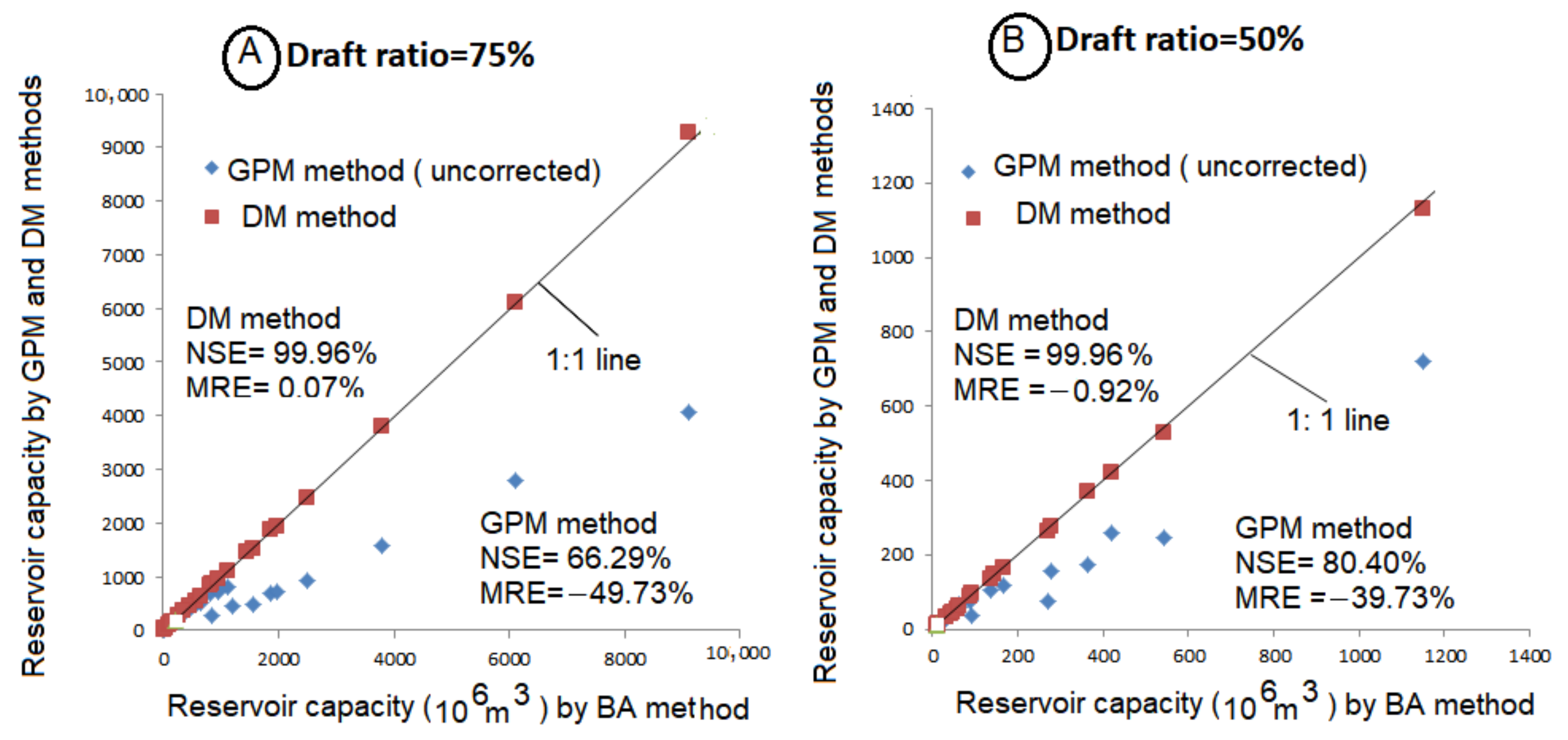
4.3. Inter-Comparison of Reservoir Capacity (CR) for Rivers with Dependent Flows

The computations of CR in rivers of group B were carried out similarly to the rivers in group A and are shown in Table 4. An important point to be noted in Table 4 is that for rivers with high ρa, the GPM-based values are substantially smaller compared to those based on the BA estimates. It is interesting to note that even for dependent annual flows, the BA and DM-based methods are comparable (columns 4, 5; 8, 9). The divergence between the GPM and the BA estimates is portrayed (diamond points) in Figure 3A,B, whereas the DM estimates against the BA estimates (square points) match much better in the graphical plots. The relevant statistics for NSE and MRE are also displayed in these figures.
For the dependent flows, it can be noted that NSE between the BA and the DM estimates are quite high (>99%), as portrayed in Figure 3A,B. Likewise, the MER values are low (=−0.92%). On the contrary, for the auto-correlated annual flows, these statistics between the GPM and the BA methods are very discouraging, respectively, with NSE ≈ 66% and 80 % and MER ≈ −50% and −40%. Such large values of MER are well reflected in the remarkable departure of diamond points in Figure 3A,B from the 1:1 line. It should be borne in mind that the BA and the DM methods (in monthly sequences) account for the seasonality and persistence effects in their algorithms, regardless of the persistence in the annual sequences. In the GPM method, the annual flow sequences are assumed to be independent, even though the monthly sequences within a year could be dependent. That is why, for the autocorrelated annual flows, the GPM method results in low estimates of the reservoir capacity (CR). These estimates must be corrected because it is well-known that autocorrelation increases the storage requirement of the reservoirs [1,2]. To this end, McMahon (1976) [17] presented correction factors (CFs) graphically based on the correlation using the reservoir capacity of the BA method as a reference value. The work was further extended by Srikanthan and McMahon (1985) [24], who carried out extensive simulation studies and developed curves displaying the correction factors (CFs) as a function of ρa, draft ratio (α), and storage ratio (ratio of storage with zero ρa to MAF) and are documented in [3].
Table 4. Comparison of estimates of reservoir capacity using GPM, BA, and DM methods at significant autocorrelation (ρa, signifying dependence) in the annual flows.
River # as Shown in Table 1, Figure 1Reservoir Capacity (CR, 106 m3) at Draft Ratio = 0.75Reservoir Capacity (CR, 106 m3) at Draft Ratio = 0.50
PF (%)GPMBADMParameters of DM MethodGPMBADMParameters of DM Method
12345678910
[2] Beaver cva = 0.72, ρa = 0.36, N = 6510.0450.0, 810.01200.01180.0MT1, Φ = 0.24(2)116.0, 118.3165.0166.0MT0, Φ = 0.70(2) *
5.0677.0, 1360.81860.01880.0MT1V, Φ = 0.55(2)175.0, 180.3363.0368.0MT0V, Φ = 0.61(2)
2.5936.0, 2059.22510.02460.0MT1V, Φ = 0.25(2)244.0, 253.8541.0530.0MT1, Φ = 0.66(2)
[3] Churchill cva = 0.37, ρa = 0.59, N = 5710.01580.0, 3175.83800.03790.0MT1, Φ = 0.71(3)65.0, 71.564.0nana
5.02800.0, 5684.06100.06100.0MT1, Φ = 0.27(3)260.0, 397.8420.0423.0MT0, Φ = 0.45(1)
2.54080.0, 8445.69100.09276.0MT1, Φ = 0.66(3)720.0, 1188.01150.01130.0MT0V, Φ = 0.25(3)
[4] Sturgeon cva = 0.43, ρa = 0.62, N = 3510.0286.0, 606.3850.0863.0MT1, Φ = 0.38(3)11.5, 21.912.0nana
5.0497.0, 804.31550.01530.0MT1V, Φ = 0.58(3)38.0, 76.493.097.5MT0V, Φ = 1.0(3)
2.5712.0, 1780.01970.01940.0MT0, Φ = 0.30(3)74.0, 162.8270.0265.0MT1, Φ = 0.83(3)
[5] Islands, cva = 0.28 ρa = 0.27, N = 4610.0282.0, 513.0280.0273.0MT0, Φ = 0.78(3)10.0, 18.010.0naMT1, Φ = na(3)
5.0490.0, 950.6572.0547.0MT1, Φ = 0.67(3)40.2, 73.244.042.2MT0, Φ = 0.1(3)
2.5 682.0, 1091.2830.0826.0MT1, Φ = 0.31(3)74.0, 117.088.087.3MT0, Φ = 0.20(3)
[6] Gods, cva = 0.28 ρa = 0.36, N = 46 10.0390.0, 393.9470.0444.0MT0V, Φ = 0.77(3)nananana
5.0816.0, 1003.71123.01110.0MT1, Φ = 0.84(3)14.5, 23.020.0nana
2.51480.0, 1998.01440.01470.0MT1, Φ = 0.61(3)147.0, 188.2145.0146.0MT0, Φ = 0.20(3)
[7] English, cva = 0.32, ρa = 0.20, N = 9910.0320.0, 329.6354.0351.0MT1, Φ = 0.92(3)49.0, 56.4 57.0 55.0MT0, Φ = 0.90(3)
5.0505.0, 681.8645.0643.0MT1, Φ = 0.61(3)107.0, 123.0136.0134.0MT0, Φ = 0.05(3)
2.5712.0, 996.9960.0960.0MT1, Φ = 0.28(3)157.0, 175.8280.0274.0MT1, Φ = 0.66(3)
[8] Neebing, cva = 0.37,
ρa = 0.20, N = 66,
N = 66
10.021.0, 29.422.022.0MT1V, Φ = 0.95(3)10.4, 12.0 9.3 9.1MT1, Φ = 0.61(3)
5.028.0, 40.630.030.0MT1, Φ = 0.60(3)10.3, 11.912.212.0MT1, Φ = 0.38(3)
2.533.8, 52.4039.038.0MT1, Φ = 0.28(3)11.4, 12.815.015.0MT0V, Φ = 0.42(3)
[13] Beaurivage, cva = 0.26, ρa= 0.19, N = 7510.092.0, 103.092.091.1MT0V, Φ = 0.24(3)33.0, 35.333.033.0MT0, Φ = 0.58(3)
5.0118.0, 139.2117.5116.0MT1, Φ = 0.25(3)44.0, 48.047.046.0MT1, Φ = 0.49(3)
2.5140.0, 182.0149.0147.0MT0V, Φ = 0.46(3)58.5, 64.361.560.7MT1, Φ = 0.21(3)
Asterisk (*) number within parentheses indicates truncation level on SHI sequences such as 2 means SHIm, 3 means SHIav. MT1 MT0, MT1V and MT0V are explained in Table 4. “na” means not applicable as the method under this column did not yield the CR Values. For example, for the Gods River, no method resulted in CR values as they were too low, and the method could not compute the needed values.
These correction factors (CFs) were interpolated from the graphs documented in [3] and are shown in Table 5 (values titled as lit which means literature). It can be seen that the correction factors range from 2.18 to 3.12 for rivers with high ρa at the draft ratio equal to 0.75 and are smaller in the range from 1.0 to 1.35 at the draft ratio equal to 0.5. It may further be noted that the CFs are not far from 1 when the draft ratio is equal to 0.5, meaning that CR estimates are closer to the case of independent flows regardless of high ρa. In other words, at low draft ratios (<0.5), CR values based on the GPM method may not require any corrections, even for correlated annual flows.
It may be borne in mind that CFs values are a function of storage ratio, i.e., (the ratio of the GPM storage/µa). The storage ratio can also be computed for the BA-based storage values, i.e., (BA storage/µa). The storage ratios so computed are shown in bold numerals (columns 5 and 9, Table 5). Using these values of CFs (columns 6 and 10, Table 5) as multipliers, the new CR values were computed and are summarized in bold numerals (Table 4) along with the uncorrected values of CR.
Table 5. Correction factors (CF) for reservoir capacity (CR in 106 m3) using the GPM method at significant lag-1autocorrelation (ρa, i.e., dependence) in the annual flows.
River # as Shown in Table 1, Figure 1PF (%)Reservoir Capacity (CR, 106 m3) Draft Ratio = 0.75Reservoir Capacity (CR, 106 m3) Draft Ratio = 0.50
GPMBA Ratio CRaCF (lit) *CF (ob)GPMBARatio CRaCF (lit) *CF (ob))
123456789101112
[2] Beaver
µa = 592.5 × 10⁶ 
ρa= 0.36, cva = 0.72
10.0450.01200.00.76, 2.031.80 *2.67116.0165.00.20, 0.281.021.42
5.0677.01860.01.14, 3.142.012.75175.0363.00.30, 0.611.032.07
2.5936.02510.01.58, 4.232.202.68244.0541.00.41, 0.581.042.21
[3] Churchill
µa = 9345.0 × 106, ρa = 0.59, cva = 0.37
10.01580.03800.00.17, 0.412.012.4165.064.00.007, 0.011.100.98
5.02800.06100.00.30, 0.652.032.18260.0420.00.028, 0.061.531.62
2.54080.09100.00.44, 0.972.072.23720.01150.00.078, 0.121.651.60
[4] Sturgeon
µa = 1479.5 × 106 
ρa = 0.62, cva = 0.43
10.0286.0850.00.19, 0.572.122.9711.512.00.008, 0.0081.901.04
5.0497.01550.00.34, 1.052.303.1238.093.00.026, 0.0622.012.45
2.5712.01970.00.48, 1.332.502.7774.0270.00.050, 0.182.203.65
[5] Islands lake
µa = 2718.1 × 106, ρa = 0.27, cva = 0.28
10.0282.0280.00.10, 0.101.820.9910.010.00.004, 0.0041.801.00
5.0490.0572.00.18, 0.211.941.1740.244.00.015, 0.0161.821.09
2.5682.0830.00.25, 0.311.601.2274.088.00.027, 0.0321.581.19
[6] Gods
µa = 4875.5 × 106, ρa = 0.36, cva = 0.28
10.0390.0470.00.08, 0.101.011.21nananana **na
5.0816.01123.00.17, 0.231.231.3814.520.00.003, 0.0041.211.38
2.51480.01440.00.30, 0.301.350.97147.0145.00.03, 0.031.280.99
[7] English
µa = 1846.4 × 106 
ρa = 0.20, cva = 0.32
10.0320.0354.00.17, 0.191.031.1149.057.00.026, 0.0311.011.16
5.0505.0645.00.27, 0.351.351.28107.0136.00.056, 0.0741.051.27
2.5712.0960.00.38, 0.521.401.35157.0280.00.082, 0.151.101.78
[8] Neebing
µa = 51.1 × 10⁶ 
ρa = 0.20, cva = 0.37
10.021.022.00.41, 0.431.401.0510.49.30.20, 0.181.150.89
5.028.030.00.55, 0.591.451.0710.312.20.20, 0.241.151.18
2.533.839.00.66, 0.761.551.1511.415.00.22, 0.291.121.32
[13] Beaurivage
µa = 447.6 × 10⁶ 
ρa = 0.19, cva = 0.27
10.092.092.00.21, 0.211.121.0033.033.00.074, 0.741.071.00
5.0118.0117.50.27, 0.271.181.0044.047.00.10, 0.111.091.07
2.5140.0149.00.31, 0.331.301.0658.561.50.13, 0.141.101.05
Asterisk (*) refers to the values of CF as shown in the graphical plots in the literature, i.e., in [13], † refers to the CF values computed as the ratio of CR (BA)/CR (GPM), i.e., column 4/column 3. Asterisk (**) denotes “na” (not applicable), which means CR values were not yielded by the respective methods and neither were CFs.
The graphs were plotted between new CR (corrected values) against the BA-based values and are depicted in Figure 4A,B. It can be noted that by involving the correction factor, the CR values improved, but there is still a significant departure from the BA-based estimates. Though the NSE increased (91% and 97.60%), but the MER was still high (−16.15% and −7.85%). This was also noted in the illustrative example of the Sturgeon River, as presented in Appendix A. Taking the BA estimates as the reference values, the corrected GPM values display considerable divergence, which is well corroborated by Figure 4A,B. This alludes to the fact that there is a need to rework these correction factors at low storage ratios at a smaller interval of α and ρa through a simulation exercise. As an illustration, these values of CFs were computed as the ratio of CR by the BA and by the GPM methods and are shown in italics (columns 7 and 11, Table 5). These values of the CFs named “ob” (observed) are larger than cited in the literature and thus warrant a need to rework them. Further work on this aspect was conducted by Phatarfod (1986) [30], who derived mathematical expressions which are demanding in comprehension sense and need further simplification by practicing users. The observed CF values can be linked to the results based on the work of Phatarfod [30]. This aspect of the investigation can form a subject of a separate study and is therefore not further explored in this paper.
From the analysis presented in this paper, it is clear that the GPM method is satisfactory for the rivers with little annual autocorrelation, particularly when data are scant and, at times, discontinuous. The method seems less promising for the rivers, which are ridden with significant annual autocorrelations, such as in Canadian prairies. The rivers in Canadian prairies tend to have significant annual lag-1 autocorrelation, ρa (>0.20), and the CR estimates need correction through multiplication by accurate values of CFs. Presently, such values are interpolated from the published literature and therefore are only rough estimates. Evolving the accurate values of CFs using simulation is fairly involved and not easily obtained. On the contrary, the BA and the DM methods can be used without any hassles as long as the monthly streamflow data of 30 years or so are available in a continuous format and without a break. The algorithms of these methods are designed to account for the first-order persistence in the monthly sequences, and no CFs are involved in the estimation of CR. The DM method requires the standardization of the data resulting in SHI sequences. In the Canadian rivers, the SHI sequences tend to follow the gamma pdf, which should be normalized using the Wison–Hilfirty transformation as documented in [27]. All the calculations should be conducted in the normalized domain. However, Sharma and Panu [28] noted that the transformation in the normalized probability domain made insignificant improvements in the estimates of CR compared to the estimation using the SHI sequences in the gamma probability domain itself. In other words, statistically standardized monthly flows designated as SHI can be used for Markov Chain modelling of drought lengths and correspondingly the drought magnitudes as demonstrated in the present analysis. This simple shortcut is sufficiently accurate for the Canadian rivers in which the monthly flow sequences follow the Gamma probability distribution. In other words, the monthly streamflow sequences can be treated as normally distributed in the DM method, though they are mildly skewed, falling in the region of the Gamma pdf.
In the present analysis, two draft ratios, viz. 75% and 50%, were used. There are situations when a draft ratio as low as 30% may require consideration for environmental and/or economic reasons. Under such situations, all the above methods tend to fail, particularly at the PF levels of 10% and 5%, which yield unreliable estimates of the CR. While confronted with such circumstances, the values of CR should be estimated at the PF level of 2.5% or less (say 0%), and the CR values so estimated can be used as design values at all PF levels. In other words, recourse should be taken to the sequent peak algorithm (SPA), which provides the conservative values of CR [5] with no consideration of PF.

5. Conclusions

Based on the study using the Canadian rivers with wide diversity in terms of annual lag-1 autocorrelation (ρa) and coefficient of variation (cva), the following conclusions can be derived.
  • For the analysis using the GPM method, 15 zones in a reservoir are sufficient to yield reliable estimates of the reservoir capacity.
  • The estimates of the reservoir capacity (CR) by the BA and the DM methods in this study were found to be nearly equal to each other for all values ρa and cva, which implies that the DM method is a competent substitute for the BA method.
  • In the DM method, which requires the standardized monthly data, i.e., the SHI sequences, the Markov chain order 1 (MC1) or MC0 model yielded the drought lengths, which when multiplied by drought intensity, resulted in the drought magnitudes. The drought magnitude (MT) multiplied by the average standard deviation of 12 months (σav) resulted in satisfactory estimates of reservoir capacity (CR). Both the BA and the GPM methods can be implemented on the non-standardized monthly flow sequences.
  • For annual flows with ρa < 0.20, the estimates of reservoir capacity (CR) by the GPM method were found in parity with the estimates of the BA or DM methods. The BA method, being simplest in terms of calculation rigor, enjoys a slight edge over the DM and the GPM methods.
  • The estimates of reservoir capacity (CR) tend to become smaller in the GPM method when the values of ρa > 0.20 or become remarkably low with high values of ρa, say 0.5 or greater. These low values of CR can be improved by invoking the correction factors as a multiplier while using the available graphical values from the literature. However, there is a need to further refinement of the correction factors (CFs).

Author Contributions

T.C.S. and U.S.P. collaboratively accomplished various tasks related to this manuscript, including draft preparation and finalization of the manuscript for journal publication, such as conceptualization and development of the methodology, and data collection and data analysis. All authors have read and agreed to the published version of the manuscript.

Funding

This research received no external funding.

Data Availability Statement

Not applicable.

Acknowledgments

The partial financial support of the Natural Sciences and Engineering Research Council of Canada for this paper is gratefully acknowledged.

Conflicts of Interest

No potential conflict was reported by the authors.

Appendix A

An Illustration of the Computational Procedure for the GPM on the Sturgeon River

The case of the Sturgeon River with an assumed value of the reservoir capacity (CR) = 496 × 106 m3 for PF = 0.05. The lag-1 autocorrelation at the annual scale, ρa = 0.62. Number of zones in the reservoir, k = 15. Volume in each zone = 496/(15−2) = 38.15 × 10 6 m3, with first and last zones having volume = 0 m3. The cumulative volume in zones 0 through 14 can be computed as follows.
Table A1. Volume of water in each zone (106 m3).
Zone0 1234567891011121314
Max vol.038.1576.30114.46152.62190.77228.92267.08305.23343.38381.54419.67457.85496.0496.0
Min. vol.0 038.1576.30114.46152.62190.77228.92267.10305.23343.38381.49419.69457.85496.0
Table A2. Monthly failure tracking.
Zone01234567891011121314
nf117104796452413323191496321
pf0.279 0.2480.1880.1520.1240.100 0.077 0.0560.0450.0330.0210.0140.0070.0050.002
Table A3. Construction of transitional matrix of the frequency of common occurrences.
Zone01234567891011121314
0998775555533211
1112213000020110
2220110300002012
3213111033000200
4010211100000020
5201021111300002
6351102111030000
7115221311103000
8000411033110300
9000041100111032
10000004111311101
11110000422142222
12001000033103222
13100100000332433
14131414141515151515161718182020
total353535353535353535353535353535
Note: The above table shows starting zone (January, zt) on the X-axis and the finishing zone (December, zt+1) on the Y-axis. For example, the intersection of the abscissa 5 and the ordinate 6 is 2, which means there are 2 instances or occasions when the starting zone(January) was 5 and the finishing zone(December) was 6. Likewise, the intersection of abscissa 9 and ordinate 14 is 16, meaning that there are 16 occasions in which January storage was in zone 9, and it ended in zone 14 in December.
Table A4. Construction of transitional probability matrix (TPM).
Zone01234567891011121314
00.2570.2570.2290.2000.20.1430.1430.1430.1430.1430.0860.0860.0570.0280.028
10.0280.0280.0570.0570.0280.08600000.05700.0280.0280
20.0570.02800.0280.02800.08600000.05700.0280.057
30.0570.0280.0860.0280.0280.02800.0860.0860000.05700
400.02800.0570.0280.0280.0280000000.0570
50.05700.02800.0570.0280.0280.0280.0280.08600000.057
60.0280.1430.0280.02800.0570.0280.0280.02800.0860000
70.0280.0280.1430.0570.0570.0280.0860.0570.0280.02800.086000
80000.1140.0280.02800.0860.0860.0280.02800.08600
900000.1140.0280.028000.0280.0280.02800.0860.057
10000000.1140.0280.0280.0280.1140.0280.0280.02800.028
110.0280.02800000.1140.0570.0570.0280.1140.0570.0570.0570.057
12000.02800000.0860.0860.02800.0860.0570.0570.057
130.028000.028000000.0860.0860.0860.1140.0860.086
140.3710.400.4000.4000.4290.4290.4290.4290.4290.4570.4570.5140.5140.5710.571
total≈1.0≈1.0≈1.0≈1.0≈1.0≈1.0≈1.0≈1.0≈1.0≈1.0≈1.0≈1.0≈1.0≈1.0≈1.0
Table A5. Construction of steady state probability matrix (squared 6 times i.e (TPM)6).
Zone01234567891011121314
00.0840.0840.0840.0840.0840.0840.0840.0840.0840.0840.0840.0840.0840.0840.084
10.0150.0150.0150.0150.0150.0150.0150.0150.0150.0150.0150.0150.0150.0150.015
20.0420.0420.0420.0420.0420.0420.0420.0420.0420.0420.0420.0420.0420.0420.042
30.0150.0150.0150.0150.0150.0150.0150.0150.0150.0150.0150.0150.0150.0150.015
40.0080.0080.0080.0080.0080.0080.0080.0080.0080.0080.0080.0080.0080.0080.008
50.0420.0420.0420.0420.0420.0420.0420.0420.0420.0420.0420.0420.0420.0420.042
60.0170.0170.0170.0170.0170.0170.0170.0170.0170.0170.0170.0170.0170.0170.017
70.0190.0190.0190.0190.0190.0190.0190.0190.0190.0190.0190.0190.0190.0190.019
80.0110.0110.0110.0110.0110.0110.0110.0110.0110.0110.0110.0110.0110.0110.011
90.0420.0420.0420.0420.0420.0420.0420.0420.0420.0420.0420.0420.0420.0420.042
100.0280.0280.0280.0280.0280.0280.0280.0280.0280.0280.0280.0280.0280.0280.028
110.0500.0500.0500.0500.0500.0500.0500.0500.0500.0500.0500.0500.0500.0500.050
120.0450.0450.0450.0450.0450.0450.0450.0450.0450.0450.0450.0450.0450.0450.045
130.0680.0680.0680.0680.0680.0680.0680.0680.0680.0680.0680.0680.0680.0680.068
140.5160.5160.5160.5160.5160.5160.5160.5160.5160.5160.5160.5160.5160.5160.516
total1.0001.0001.0001.0001.0001.0001.0001.0001.0001.0001.0001.0001.0001.0001.000
Table A6. Evaluation of failure probability.
ZoneSteady-State Probability (from Table A5)Failure Probability in Zones
(from Table 2)
Product of Probabilities
Column(2) × Column(3)
(1)(2)(3)(4)
00.2785710.0841240.023435
10.2476190.0146670.003632
20.1880950.0420070.007901
30.1523810.0148520.002263
40.1238100.0079770.000988
50.0976190.0417910.00408
60.0785710.0170310.001338
70.0547620.0190940.001046
80.0452380.0108770.000492
90.0333330.0422220.001407
100.0214290.0276460.000592
110.0142860.0495740.000708
120.0071430.0444970.000318
130.0047620.0676930.000322
140.0023810.5159470.001228
PF =sum of column (4)0.050
The above-computed value of PF = 0.05 tallies exactly with the desired value of PF = 0.05 using the trial value of CR = 496 × 106 m3, therefore, the GPM based CR = 496 × 106 m3. However, this CR must be corrected for the annual autocorrelation (ρa = 0.62) for this river. The correction factor from the graph by Srikanthan (1985) is =2.01; and thus, the actual CR = 2.01 × 496 × 106 m3 = 997.0 × 10⁶ m3.

References

  1. McMahon, T.A.; Pegram, G.G.S.; Vogel, R.M.; Peel, M.C. Revisiting reservoir storage—Yield relationships using a global streamflow database. Adv. Water Resour. 2007, 30, 1858–1872. [Google Scholar] [CrossRef]
  2. McMahon, T.A.; Vogel, R.M.; Pegram, G.G.S.; Peel, M.C.; Etkin, D. Global streamflows—Part 2: Reservoir storage yield performance. J. Hydrol. 2007, 347, 260–261. [Google Scholar] [CrossRef]
  3. McMahon, T.A.; Mein, R.G. River and Reservoir Yield; Water Resources Publications: Littleton, CO, USA, 1986; p. 149. [Google Scholar]
  4. McMahon, T.A.; Adeloye, A.J. Water Resources Yield; Water Resources Publications: Littleton, CO, USA, 2005; p. 88. [Google Scholar]
  5. Sharma, T.C.; Panu, U.S. A drought magnitude based method for reservoir sizing: A case of annual and monthly flows from Canadian rivers. J. Hydrol. Reg. Stud. 2021, 36, 100829. [Google Scholar] [CrossRef]
  6. Sharma, T.C.; Panu, U.S. Reservoir sizing at the draft Level of 75% of mean annual flow using drought magnitude-based method on Canadian rivers. Hydrology 2021, 8, 79. [Google Scholar] [CrossRef]
  7. Thomas, H.A.; Burden, R.P. Operation Research in Water Quality Management; Division of Engineering and Applied Physics, Harvard University: Cambridge, MA, USA, 1963. [Google Scholar]
  8. Loucks, D.P.; Stedinger, J.R.; Haith, D.A. Water Resources Systems Planning; Prentice-Hall: Englewood, NJ, USA, 1981; p. 33. [Google Scholar]
  9. Linsley, R.K.; Franzini, J.B.; Freyburg, D.L.; Tchobanoglous, G. Water Resources Engineering, 4th ed.; Irwin McGraw-Hill: New York, NY, USA, 1992; p. 192. [Google Scholar]
  10. Lele, S.M. Improved algorithm for reservoir capacity calculation incorporating storage-dependent and reliability norm. Water Resour. Res. 1987, 23, 1819–1823. [Google Scholar] [CrossRef] [Green Version]
  11. Nagy, T.V.; Asante-Dua, K.; Zsuffa, I. Hydrological Dimensioning and Operation of Reservoirs. Practical Design Concepts and Principles; Kluwer Academic Publishers: Dordrecht, The Netherlands, 2002; p. 192. [Google Scholar]
  12. Alrayess, H.; Zeybekoglu, U.; Ulke, A. Different design techniques in determining reservoir capacity. Eur. Water 2017, 60, 107–115. [Google Scholar]
  13. Moran, P.A.P. Probability theory of dams. Aust. J. Appl. Sci. 1954, 5, 116. [Google Scholar]
  14. Moran, P.A.P. Theory of Storage; Methuen: London, UK, 1959. [Google Scholar]
  15. Gould, B.W. Statistical methods for estimating the design capacity of dams. J. Inst. Eng. Aust. 1961, 33, 405–416. [Google Scholar]
  16. Gould, B.W. Discussion of paper by Alexander. In Water Resources Use and Management; Melbourne University Press: Melbourne, Australia, 1964; pp. 161–164. [Google Scholar]
  17. McMahon, T.A. Preliminary estimation of reservoir storage for Australian streams. Eng. Australia CE 1976, 18, 55–59. [Google Scholar]
  18. Theo, C.H.; McMahon, T.A. Evaluation of rapid reservoir yield procedure. Adv. Water Resour. 1982, 5, 202–215. [Google Scholar]
  19. Parks, Y.P.; Farquharson, F.A.K.; Plinston, D.T. Use of the Gould probability matrix method of reservoir design in arid and semi-arid regions. In Proceedings of the Sahel Forums on the State-of-the-Art of Hydrology and Hydrogeology of the Arid and Semi-Arid Areas of Africa, Ouagadougou, Burkina Faso, 7–12 November 1988; Demiossie, M., Stout, E., Eds.; IWRA: Urbana, IL, USA, 1989; pp. 129–136. [Google Scholar]
  20. Otieno, F.A.O.; Ndiritu, J.G. The effect of serial correlation on reservoir capacity using the modified Gould probability matrix method. Water S. Afr. 1997, 23, 63–70. [Google Scholar]
  21. Ragab, R.; Austin, B.; Modinis, D. The HYDROMED model and its application to semi-arid and Mediterranean catchments with hilly reservoirs 3: Reservoir storage capacity and probability of failure model. Hydrol. Earth Syst. Sci. 2001, 5, 563–568. [Google Scholar] [CrossRef] [Green Version]
  22. Ibn Abubakar, B.S.U. Assessment of reservoir storage in a semi-arid environment using the Gould probability matrix method. Afr. Res. Rev. 2008, 2, 35–45. [Google Scholar]
  23. Kraus, A.; Rice, M.; Watson, G. Comparative Analysis of Reservoir Sizing Inclusive of the Gould Probability Matrix Method; An unpublished undergraduate technical report of the civil engineering; Faculty of Engineering, Lakehead University: Thunder Bay, ON, Canada, May 2022. [Google Scholar]
  24. Srikanthan, R.; McMahon, T.A. Gould’s Probability matrix method the annual autocorrelation problem. J. Hydrol. 1985, 77, 135–139. [Google Scholar] [CrossRef]
  25. Environment Canada. HYDAT CD-ROM Version 96-1.04 and HYDAT-ROM User’s Manual. In Surface Water and Sediment Data; Water Survey of Canada: Gatineau, QC, Canada, 2020. [Google Scholar]
  26. Dracup, J.A.; Lee, K.S.; Paulson, E.G. On the statistical characteristics of drought events. Water Resour. Res. 1980, 16, 289–296. [Google Scholar] [CrossRef]
  27. Sharma, T.C.; Panu, U.S. A semi-empirical method for predicting hydrological drought magnitudes in the Canadian prairies. Hydrol. Sci. J. 2013, 58, 549–569. [Google Scholar] [CrossRef] [Green Version]
  28. Sharma, T.C.; Panu, U.S. Modelling of hydrological drought durations and magnitudes: Experiences on Canadian streamflows. J. Hydrol. Reg. Stud. 2014, 1, 92–106. [Google Scholar] [CrossRef] [Green Version]
  29. Nash, J.E.; Sutcliffe, J.V. River flow forecasting through conceptual models: Part 1—A discussion of Principles. J. Hydrol. 1970, 10, 282–290. [Google Scholar] [CrossRef]
  30. Phatarfod, R.M. The Effect of serial correlation on reservoir size. Water Resour. Res. 1986, 22, 927–934. [Google Scholar] [CrossRef]
Figure 1. Location of river gauging stations across Canada (source Environment Canada).
Hydrology 10 00053 g001
Figure 2. Plots of CR based on the GPM and DM methods versus the BA method for independent annual flows. (A) Draft ratio = 75%, (B) Draft ratio = 50%.
Hydrology 10 00053 g002
Figure 3. Plots of CR based on GPM (uncorrected) and DM methods against BA method for annual flows. (A) Draft ratio = 75%, (B) Draft ratio = 50%.
Hydrology 10 00053 g003
Figure 4. Plots of CR based on the GPM (corrected) and the DM methods against the BA method for dependent annual flows. (A) Draft ratio = 75%, (B) Draft ratio = 50%.
Hydrology 10 00053 g004
Table 2. Comparison of the estimates of reservoir capacity using 15 and 20 zones.
River and
Relevant Parameters
CR (106 m3) at Draft Ratio = 0.75CR (106 m3) at Daft Ratio = 0.50
Nz = 20Nz = 15Nz = 20Nz = 15
PF Level (%)PF Level (%)PF Level (%)PF Level (%)
1052.51052.51052.51052.5
12345678910111213
Bow River,
cva = 0.13, ρa = 0.06
290.0 321.0337.2290.0 321.0339.0133.0150.0160.0 133.0 149.0 160.5
Beaver River,
cva = 0.72, ρa = 0.36
442.0690.0935.0450.0677.0936.0115.0175.5246.0116.0175.0244.0
Sturgeon River,
cva = 0.43, ρa = 0.63
287.0500.0712.0286.0497.0712.011.538.074.811.538.074.0
Islands lake River,
cva = 0.28, ρa = 0.27
280.0493.0680.0282.0490.0682.010.040.074.010.040.274.0
English River
cva = 0.32, ρa = 0.20
322.0500.0712.0320.0505.0712.050.0107.0158.049.0107.0157.0
Beconcour River
cva = 0.20, ρa = 0.03
176.5235.0281.0177.0234.0281.060.386.7112.860.386.7112.8
U. Humber River cva = 0.13, ρa = 0.18277.0358.0430.0277.0358.0429.0103.0142.0185.0103.0142.0185.0
NOTE: The bold numerals show the discrepancy in the estimates of CR but they are within 2% of each other. Otherwise, all other values are much less than 2%.
Table 3. Comparison of estimates of reservoir capacity using GPM, BA, and DM methods with insignificant autocorrelation (ρa, i.e., independence) in the annual flows.
River # as Shown in Table 1, Figure 1Reservoir Capacity (CR, 106 m3) at Draft Ratio = 0.75Reservoir Capacity (CR, 106 m3) at Draft Ratio = 0.50
PF (%)GPMBADMParameters on DM MethodGPMBADMParameters on DM Method
12345678910
[1] Bow River, cva = 0.13, ρa = 0.06, N = 11010.0290.0286.0283.0MT1V, Φ = 0.64(1)133.0133.0128.0MT1, Φ = 0.35(1) *
5.0321.0323.0317.0MT1V, Φ = 0.54(1)149.0151.0147.0MT1, Φ = 0.21(1)
2.5339.0343.0336.0MT1V, Φ = 0.49(1)160.5164.8160.0MT1, Φ = 0.12(1)
[9] Pic River, cva = 0.24, ρa = 0.13, N = 5010.0340.0325.0317.0MT1, Φ = 0.48(3)134.0133.0126.0MT1, Φ = 0.78(3)
5.0480.0490.0483.0MC1, Φ = 0.04(3)193.0195.0192.0MT1, Φ = 0.45(3)
2.5579.0588.0578.0MC1V, Φ = 0.61(3)255.0270.0255.0MT1, Φ = 0.13(3)
[10] Pagwa- chaun, cva = 0.25 ρa = 0.06, N = 5310.0208.0182.0177.0MT1, Φ = 0.43(3)108.075.073.3MT1, Φ = 0.69(3)
5.0237.0240.0239.0MT1, Φ = 0.12(3)127.0108.0106.0MT1, Φ = 0.38(3)
2.5250.0300.0296.0MT1V, Φ = 0.62(3)130.0152.0150.0 MT0V, Φ = 0.20(3)
[11] Goulis cva = 0.24, ρa = 0.13,
N = 53
10.0100.099.098.0MT1, Φ = 0.62(3)31.531.030.2MT1, Φ = 0.93(3)
5.0135.0138.5136.0MT1, Φ = 0.35(3)44.545.045.4MT1, Φ = 0.69(3)
2.5166.0169.0167.0MT1, Φ = 0.13(3)65.066.064.4MT1, Φ = 0.39(3)
[12] Becancour cva = 0.20, ρa = 0.03, N = 5310.0177.0175.0172.0MT1, Φ = 0.57(3)60.361.261.1MT1, Φ = 0.88(3)
5.0234.0230.0231.0MT1, Φ = 0.32(3)86.786.786.03MT1, Φ = 0.64(3)
2.5281.0275.0281.0MT1, Φ = 0.12(3)112.8114.0112.1MT1, Φ = 0.40(3)
[14] Lepraue
cva = 0.22, ρa = 0.10, N = 101
10.039.938.035.5MT1, Φ = 0.69(3)8.013.113.4MT0, Φ = 0.67(3)
5.045.048.047.2MT1, Φ = 0.50(3)16.020.020.4MT1, Φ = 0.64(3)
2.561.561.760.8MT1, Φ = 0.28(3)24.227.527.7MT1, Φ = 0.40(3)
[15] U. Humber cva = 0.13, ρa = 0.18, N = 6810.0277.0277.0275.0MT0, Φ = 0.23(3)103.0104.098.9MT1, Φ = 0.32(3)
5.0358.0355.0351.0MT1, Φ = 0.20(3)142.0136.0134.0MT1, Φ = 0.52(3)
2.5429.0412.0402.0MT0V, Φ = 0.63(3)185.0184.5179.0MT1, Φ = 0.20(3)
[16] Torrent cva = 0.15, ρa = 0.18, N = 6110.097.097.095.3MT1, Φ = 0.62(1)35.234.532.5 MTV0, Φ = 0.90(1)
5.0125.0125.0122.0MT1, Φ = 0.43(1)49.049.048.1MT1, Φ = 0.80(1)
2.5146.0147.0146.0MT1, Φ = 0.75(1)63.063.059.7MT1, Φ = 0.46(1)
Asterisk (*) number within parentheses indicates truncation level on SHI sequences such as 1 means SHIo, 3 means SHIav. MT1 and MT0 mean the drought magnitude is based on Markov chain (MC) order 1 or 0 multiplied by the mean of drought intensity (Id). MC1V and MC0V are based on both the mean and variance of the drought intensity (Id).
Disclaimer/Publisher’s Note: The statements, opinions and data contained in all publications are solely those of the individual author(s) and contributor(s) and not of MDPI and/or the editor(s). MDPI and/or the editor(s) disclaim responsibility for any injury to people or property resulting from any ideas, methods, instructions or products referred to in the content.

