Article

Spatial Evaluation of a Hydrological Model on Dominant Runoff Generation Processes Using Soil Hydrologic Maps

1
Department of Physical Geography, University of Trier, 54286 Trier, Germany
2
Hydrology Department, University of Trier, 54286 Trier, Germany
*
Author to whom correspondence should be addressed.
Hydrology 2023, 10(3), 55; https://doi.org/10.3390/hydrology10030055
Submission received: 6 January 2023 / Revised: 11 February 2023 / Accepted: 17 February 2023 / Published: 22 February 2023

Abstract

:
The aim of this study was to simulate dominant runoff generation processes (DRPs) in a mesoscale catchment in southwestern Germany with the physically-based distributed hydrological model WaSiM-ETH and to compare the resulting DRP patterns with a data-mining-based digital soil map. The model was parameterized by using 11 Pedo-transfer functions (PTFs) and driven by multiple synthetic rainfall events. For the pattern comparison, a multiple-component spatial performance metric (SPAEF) was applied. The simulated DRPs showed a large variability in terms of land use, applied rainfall rates, and the different PTFs, which highly influence the rapid runoff generation under wet conditions.

1. Introduction

Distributed physically-based hydrological models have been the mainstream in the community of hydrological modelers, providing significant insights into understanding and predicting hydrological fluxes and states [1,2]. Based on the rainfall–runoff response, these models account for the spatio-temporal dynamics of hydrological processes at various scales [3,4,5,6]. Modeling the interplay of hydrological processes in a spatially distinct manner provides the required tool to tackle the issues at hand driven by global climate change and land use intensification. The capability of a model to predict the spatial variabilities of hydrological processes, however, poses evident challenges to its modeling structure. Thereby, considering the complex feedbacks between the hydrological processes that drive spatial variability, distributed hydrological model applications are a challenge for spatial pattern-oriented evaluations [7,8,9]. The spatial predictability of distributed model output can only be thoroughly verified when evaluating the outputs against spatial observations [9,10], whereas, in particular, discharge data at the catchment outlet does not provide sound information about the spatial distribution of runoff processes within the catchment [11].
Changes in the underlying land surface conditions caused by land use, soil types, geological, and topographical factors may alter the spatial patterns of runoff generation processes in a catchment area, which might then cause extreme flood or drought events. Such events may further influence the subsequent processes that govern the runoff response of a region, particularly in smaller catchments. For example, for water resource management and early flood warning, it is important to conduct quantitative measurements of the effects of urbanization on surface runoff. A recent study approached runoff fluctuations in an urban region using GIS and remote sensing technologies as well as the SCS-CN model [12]. It was found that within the period of 15 years, the region experienced a significant growth of urban impervious areas and a notable decline in vegetated land cover, being the predominant drivers of surface runoff change. The rise in surface runoff was found to be positively correlated to the growth in urbanization and negatively correlated to the decreased vegetation cover. Another study analyzed the effects of land use change on runoff production by using the SCS-CN approach, remote sensing data, and GIS tools, where runoff was predicted from precipitation, land use, and hydrological soil groups using the SCS-CN model [13]. According to another study, the influence of different land use covers on the soil hydraulic properties was investigated, and consequently, different soil hydrological behaviors to heavy storms were found, and therefore, different runoff productions were observed [14].
A well-performing hydrological model of a given catchment is in essence a virtual reflection of how the runoff generation processes vary spatially and temporally and switch between major flow mechanisms (i.e., surface runoff, subsurface flow, or base flow) [15]. While various runoff processes may occur on a site, only the dominant processes most likely contribute to the total runoff of the catchment and are significantly dependent on the site characteristics and the nature of the precipitation event [16,17]. For instance, relatively flat areas adjacent to the flow channel are disposed to faster saturation (i.e., even during slight precipitation events) and can quickly transfer water to the river network, which generally results in a fast runoff response (e.g., saturation overland flow). In contrast, runoff responses from hillslope zones are relatively slower, even during higher intensity rainfall events, and may largely contribute to processes such as interflow. Therefore, models that correctly discern the spatial variability of dominant runoff processes (DRPs) and identify flow pathways consistent with spatial observations can serve as tools to make predictions and test the hypotheses of the controls on hydrological responses [18,19,20,21,22]. The spatial information of DRPs in a catchment allow for a thorough evaluation of how a model represents the spatial distribution of runoff generation and the contributing areas under different rainfall characteristics and initial catchment conditions. The various mapping approaches for DRPs differ regarding the time and data required for mapping, and accordingly, the defined DRP classes might then be different [16,23,24].
While better process representations are required, it has always been quite a challenge to acquire good quality observed datasets with minimal uncertainty for hydrological model testing. Such datasets should then ideally transfer information about the changes in storage and variations in travel time distributions as a catchment wets and dries out, so that models can confidently be evaluated against the spatial distribution of runoff generation processes and the internal moisture state in catchments with different properties [25,26,27]. This highlights the principle that the model evaluation should thus make use of all sources of data available in a catchment area [25,28]. Antonetti et al. (2019) applied multiple DRP maps to incorporate the knowledge on DRPs into hydrological modeling. They presented divergent catchment reactions in terms of DRPs to precipitation events for flash flood predictions. They implemented synthetic runoff simulations to assess the sensitivity of the hydrograph to the mapping approach and found that simulations following the simplified procedures resulted in the strongest deviations from the reference map. Furthermore, in the Nahe catchment in Rhineland-Pfalz, Haag et al. (2016) [29] also integrated spatially distributed information on DRPs based on the classification of Scherrer and Naef (2003) [30] into LARSIM (large area runoff simulation model) for operational flood forecast [31] and applied different soil parameterizations corresponding to DRPs in the catchment area.
Thereupon, in the present study, we attempted to utilize an available soil hydrological map for the state of Rhineland-Palatinate (western Germany) from which the DRPs in a landscape unit are identified [32]. This map reflects different flow processes, which are plausible based on the site’s characteristics. In this paper, we intend to integrate this process information into rainfall–runoff model evaluation. Therefore, a methodology was developed that translates the map content into runoff classes that are consistent with the model structure in use. This would then enable spatial pattern-oriented evaluation on DRPs, for which we adopted a multiple-component spatial performance metric (SPAEF) [33]. We then defined a series of synthetic rainfall events with different intensities on a system moisture state around field capacity to assess how different rainfall intensities affect the spatial patterns of DRPs in the catchment. Furthermore, we applied 11 different Pedo-transfer functions (PTFs) to translate the information on soil properties into model parameters, since the choice of PTFs has a distinctive effect on the water balance and runoff generation [7]. Overall, this study aimed to provide a basis to understand and evaluate the observed differences in the spatial patterns of DRPs at the catchment scale and to use this information as a significant constraint in the evaluation process of a hydrological model. This would allow for the selection of behavioral model parameterizations (rather than compensating through calibration).

2. Materials and Methods
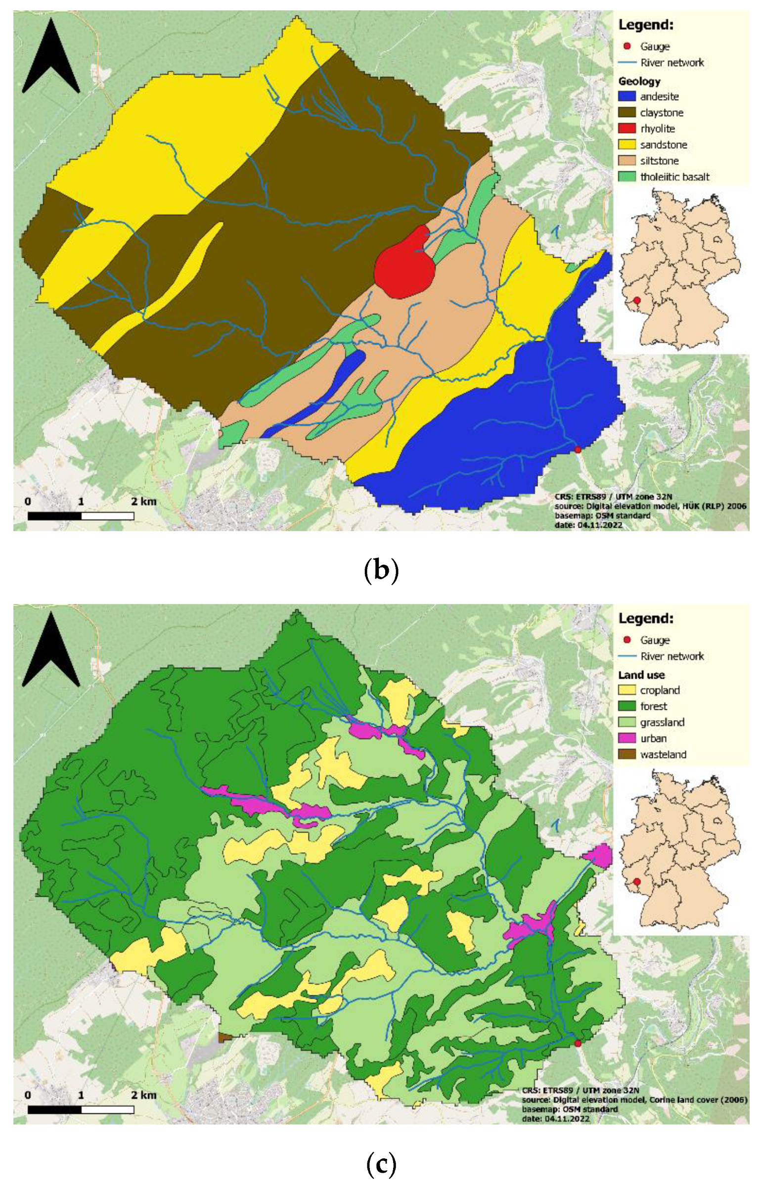
2.1. Study Area

The Kronweiler catchment in the Nahe Valley is located in the state of Rhineland-Palatinate in the southwest of Germany. The catchment, with an area of 64 km2, has a distinct river network, and the elevation ranges from 298 m a.s.l. (in the southeast) to above 720 m a.s.l. (in the north and northwest), resulting in a mean slope gradient of 8.6 and a notable altitude difference (see Figure 1a; [34]). Soil and geological information (Figure 1b) were derived from the “Hydrologische Übersichtskarte Rheinland-Pfalz” (2006). Sandstone mainly occurs in the northern parts, and siltstone underlies the southwest parts of the region. Dominant soil types are Gleyic and Humic Podzols and Cambisols.
Land use information (Figure 1c) was taken from the Corine land cover dataset (CLC, 2006), which represents forested areas as the largest land use (66%) followed by grassland (29%), cropland (3.9%), urban (0.9%), and wasteland (0.2%). While forests are patchily scattered throughout the catchment, they large cover the northern areas and the areas around the river network in the south. There are also grasslands distributed evenly over the entire area, except for the highlands in the north.

2.2. Model Setup and Parameterization

The hydrological model WaSiM (http://www.wasim.ch, accessed on 17 February 2023) was applied to analyze the water balance and runoff generation processes in the catchment. As a distributed and deterministic model, WaSiM provides physical descriptions of the involved hydrological processes. It applies Richard’s equation [35] to simulate unsaturated water fluxes in the soil and uses van Genuchten parameters [36] for the parameterization of the soil hydraulic properties. WaSiM represents the soil as a layered column. This means, for each soil horizon, that the layer thickness and water retention curve are separately defined. Every horizon within a soil profile is characterized with a specific permeability. To describe the water retention curve, estimations of the van Genuchten parameters as well as the saturated hydraulic conductivities are required (i.e., by using PTFs). The model indicates different runoff response types (fast, intermediate, slow) by simulating the three runoff components surface runoff, interflow, and base flow. A detailed description of the procedure by which the model determines the DRPs in the catchment is presented in the Section 2.4.2).
The model was set up with a spatial resolution of 50 m and a temporal resolution of 1 h. The required input time series of precipitation, temperature, relative humidity, global radiation, and wind speed were taken from the meteorological station of Dienstweiler (https://www.wetter.rlp.de/agrarmeteorologie, accessed on 17 February 2023). The pre-processing tool of WaSim-ETH TANALYS was applied to derive the necessary spatial data (e.g., slope, flow accumulation, sub-catchment structure, and stream network). The depth of the bulk density and organic matter content for each soil type and horizon were adapted considering the main land use types. The input time series of 6 years (2009–2014) was used for the model stabilization. Then, the system moisture state on 31 December 2014 represents the catchment moisture condition around field capacity.
Overall, without the interference of model calibration, the model allows for the analysis of the effects of changes in the soil hydraulic properties and rainfall event characteristics on the dominant runoff behavior of the catchment and its spatial patterns. In other words, for the purpose of this study, the exact description of the reality was of minor importance.
A combination of 11 PTFs were applied through different simulation runs to consider the effect of the different soil parameterizations by PTFs on the spatial patterns of runoff processes in the catchment. Defined PTF combinations (Table 1) determined the van Genuchten parameters (i.e., θsat, θres, n) and saturated hydraulic conductivity Ksat. Determination of the Ksat for the combinations of 1 to 7 was carried out according to the table of the Ad-hoc-AG Boden (2005) [37], while for the combinations of 8 to 10, the corresponding equations of selected PTFs were applied. The main differences among the PTFs were the underlying databases, number of considered soil samples, and the selected input predictors to the equations (i.e., soil texture is included in all PTFs as an input, but bulk density and organic matter content are not always considered in some of the PTFs). For detailed information on the following PTF combinations, see [7].

2.3. Synthetic Rainfall Events

We defined a series of synthetic rainfall events with different intensities but fixed volume to analyze their impact on the spatial patterns of DRPs in the catchment. Instead of focusing on how well the model reproduces a measured discharge, the word “synthetic” implies that the focus of this study was exclusively on the differences between the simulated patterns and patterns derived from a digital soil map. The synthetic rainfall event series had a consistent total rainfall amount of 100 mm of precipitation and accordingly, ascending rainfall durations resulted in descending intensities (Table 2). According to the available rainfall data on large precipitation events in the area, the amount of 100 mm rainfall in 3 to 10 h is realistic. In addition, this amount is high enough to force the model to reach the maximum infiltration rates and eventually produce overland flow. In other words, during the 3 up to 10 h of synthetic rainfall, the changes in the spatial distribution of surface runoff, interflow, and deep percolation were analyzed.
The simulation period was set to 7 days to consider the contribution of delayed flow processes. To ensure that no process other than the main runoff processes (i.e., overland flow, interflow, and deep percolation) was triggered within the catchment, the air humidity was set to a constant value of 100%, which prevents evaporation processes. Air temperatures above 0 °C prevent any snow contribution. This ensures that the defined precipitation amount predominantly transforms into runoff production.

2.4. Determination of Dominant Runoff Generation Process (DRP)

2.4.1. DRP by Reference Soil Hydrological Map

Information on the spatial distribution of runoff processes in a catchment can be visualized in maps discerning different types of runoff [24]. There are different mapping techniques for DRPs regarding the required time and data for mapping, and therefore, the DRP classes might be differently defined [16,23,24,30]. For the Nahe River Basin located in the state of Rhineland-Palatinate in southwest Germany, a runoff generation (reference) map is available, which also encompasses the study area Kronweiler [32]. To create this reference map, in a first step, four reference areas were mapped by experts using the mapping scheme of Scherrer (2006) [44]. In a second step, a data-driven artificial intelligence method used (i) these maps, (ii) the output from digital terrain analysis (e.g., slope, distance to stream) [45], and (iii) spatial information about geology, soil, and land use to generate the final product, a map of the dominant runoff generation processes, and the reaction time (Table 3) [46,47]. The resulting spatial structure of DRPs is plausible, for instance, if a location is close to the stream channels or on steep slopes, runoff generation is faster and overland flow or interflow, respectively, are more likely (Figure 2). If a location is dominated by permeable soils or permeable geology, deep percolation or (on slopes) interflow are more likely as dominant DRPs [32].
(1)
Saturated overland flow (SOF) describes the surface runoff, occurring when the storage capacity is exceeded due to saturation of the soil profile. The levels (or subclasses) describe the pace of the flow process from very fast (1) to delayed (2) and strongly delayed (3). Subclass SOF1 arises when the soil is saturated very fast. The subclasses SOF2 and SOF3 show an increasing saturation deficit, where saturation happens with a delay.
(2)
Subsurface flow (SSF) describes the flow processes within the soil profile, where precipitation water infiltrates through the soil surface. There, it can either be stored or continues to percolate until reaching the groundwater table. When a well-permeable soil horizon lies above a less permeable horizon, lateral subsurface runoff can also occur.
(3)
Deep percolation (DP) describes the percolation of water to deeper soil horizons.

2.4.2. Determining DRPs Using a Hydrological Model

The rainfall–runoff transformations simulated with WaSiM are represented by three runoff components. Surface runoff and interflow simulations are directly produced by the model runs, and by subtracting these runoff components from the total runoff, deep percolation can be estimated. As a result, each grid cell of the catchment area individually represents a runoff process. Here, the evaporation or other intermediate storage is not triggered. A runoff component comprising 75% of the precipitation is considered dominant. Therefore, the DRPs can be initially defined into three classes:
1 = Deep percolation is dominant;
2 = Interflow is dominant;
3 = Surface runoff is dominant.
This classification holds true if the respective runoff process is triggered from at least 75% of the total precipitation. However, when there is no runoff process with a 75% contribution rate and the runoff shares are very close to each other, two further classes can be defined considering the second largest runoff shares. Accordingly, the grid cells are assigned to the corresponding DRP classes (Table 4).
For instance, class 1.5 is assigned whenever one or more of the following conditions apply:
(1)
When interflow (IF) is greater than 50% and DP is greater than 25% at the same time, or
(2)
If DP is greater than 50% and at the same time IF is greater than 25%, or
(3)
When DP is greater than 50% and at the same time the surface runoff (SR) is greater than 25%.

2.4.3. Reclassification of the Reference Map for DRPs

A common classification must be set because the classes used for the determination of DRPs for the model simulations and those of the reference map do not match. For this purpose, the classes of the reference map were adapted to those of the simulation model. Table 5 shows the reclassification. To give an example, since class DP and DP = in the map and class 1 in the model both represent deep percolation as DRP, DP and DP = classes of the reference map were assigned to class 1.

2.5. Quantitative Evaluation of Spatial Patterns of DRPs

The accordance of the spatial patterns between the model and reference map was evaluated by using a spatial efficiency metric (SPAEF, see Equation (1)) developed by Demirel et al. (2018) [33]. The SPAEF is a multi-component statistical metric inspired by the Kling–Gupta efficiency [49] that quantifies the spatial similarity between the simulation patterns and spatial observation. The three components of the SPAEF are (i) the Pearson correlation coefficient (α); (ii) the coefficient of variation (β); and (iii) percentage of histogram intersection (γ), as follows:
Equation (1). SPAEF spatial efficiency metric formula.
SPAEF = 1 α 1 2 + β 1 2 + γ 1 2    
where
α = ρ   A ,   B ;   β = σ A μ A / σ B μ B ;   γ = j = 1 n min K j ,   L j j = 1 n K j  
where α is the Pearson correlation coefficient between A (spatial observation by the reference map) and B (simulated patterns). β is the fraction of the coefficient of variation representing spatial variability. γ is the histogram overlap for the given histograms K of the patterns of A and L of the patterns of B, each containing n bins. The spatial efficiency scale value ranges from −∞ to 1. If the value is above 0, a pattern match can be seen. The better the similarity between the patterns, the closer the efficiency metric value approaches unity.

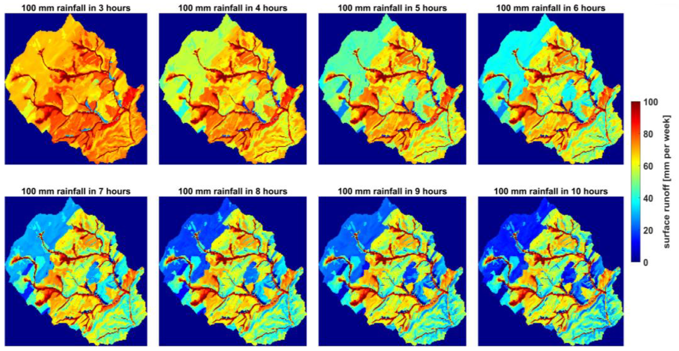
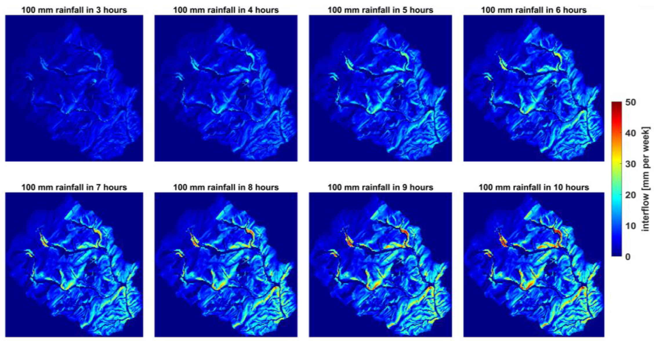
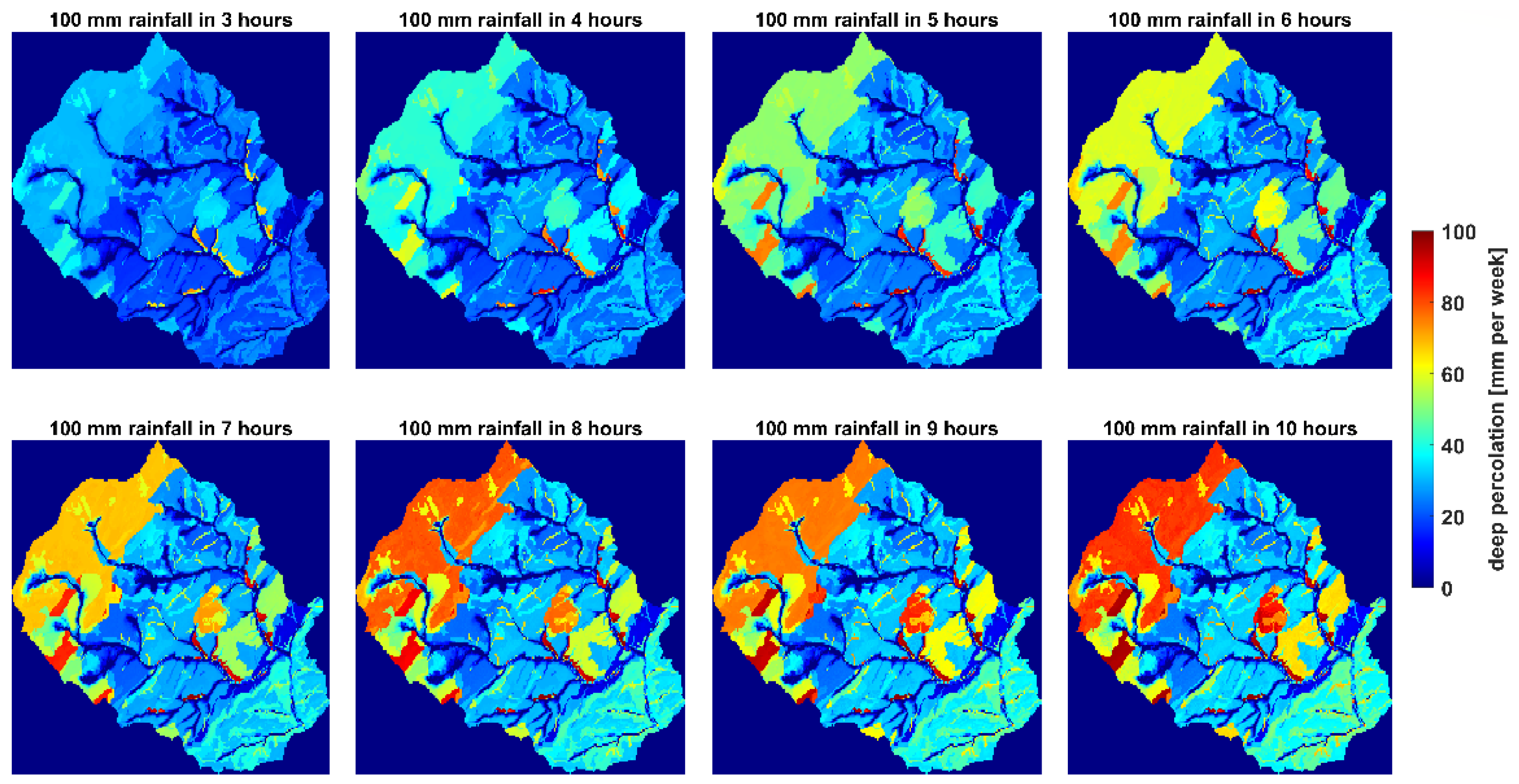
3. Effects of Rainfall Intensities on Spatial Patterns of Simulated Runoff Processes

Different rainfall intensities together with different soil hydraulic properties (i.e., derived from various PTF combinations) can be applied to simulate the runoff processes (i.e., surface runoff, interflow, and deep percolation) occurring in the catchment, and accordingly, the changes in the spatial patterns are illustrated (Figure 3, Figure 4 and Figure 5). The moisture pre-condition for the catchment system is considered as the moisture content at the root zone after an extended rainfall period, which amounts to soil water content near field capacity. Here, we present only PTF combination 5 [37,42] because it showed the highest similarity to the reference map.
A clear variability could be seen in the spatial patterns (Figure 3). For all rainfall intensities, the patterns of surface runoff with the highest values (about 80 to 100 mm) were observed in the stream channels or in the adjacent areas, except for some spots close to the channels (in blue colors), which resulted lower amounts of surface runoff. These exceptions showed a remarkable decreased runoff value of about 35 mm for the rainfall intensity of 100 mm/3 h (displayed in light blue) and continued to show lower runoff values with increasing precipitation duration until it no longer generated surface runoff for a 6 h precipitation duration and longer (displayed in darker blue colors). In general, with an increase in the precipitation duration (i.e., decreasing rainfall intensity), spatial patterns showed a significant decline in the amount of surface runoff, distinctly in the distant locations from the river courses. These patterns were particularly recognizable in the high elevations of the catchment in the north and northwest as well as in the low elevations in the south and southeast, and a sub-area in the center of the catchment.
Obviously, with an increasing rainfall duration, and therefore a decreasing rainfall intensity, the interflow amount rose (Figure 4). It can be stated that the interflow largely developed near the river courses (i.e., not in them). It is also remarkable that the interflow patterns in the catchment did not change from a precipitation duration of 6 h up to 10 h. If the total catchment is considered, the interflow usually amounted to 15–20 mm. However, interflow occasionally reached 35–50 mm in simulations with higher rainfall intensities (e.g., 100 mm in 3 and 4 h) and only in a small area close to the channels.
Total deep percolation increased mostly within the catchment, as the rainfall duration became longer (Figure 5). This overall change was markedly pronounced up to the rainfall event of 100 mm/7 h, while a further reduction in rainfall intensity did not show a clear increase in deep percolation. Under the highest rainfall intensity (i.e., 100 mm/3 h), the simulations still showed development of the spatial patterns of deep percolation in the catchment. These patterns reached amounts between 30 mm and 45 mm in deep percolation over large areas in the north, northwest, and central areas between the river courses and eastern parts of the catchment. For the lowest precipitation intensity of 100 mm/10 h, the upland areas with higher permeability transformed almost all the precipitation water into deep percolation and produced patterns with amounts of 65–90 mm. Overall, the areas developing the highest deep percolation shares corresponded to forest land use.

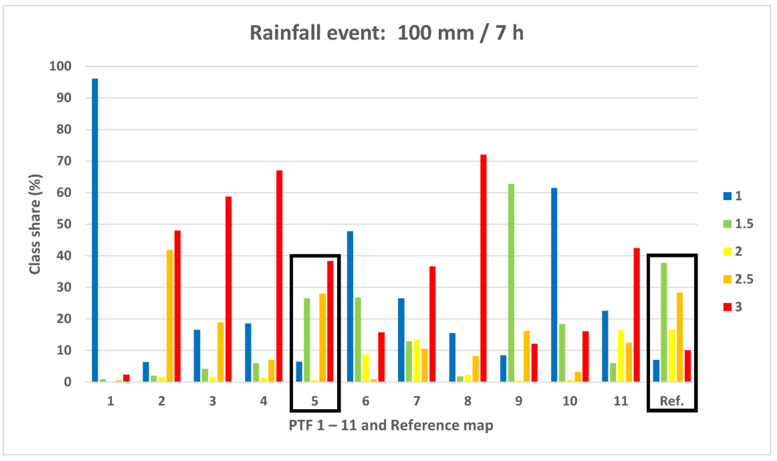
4. Spatial Evaluation of Simulated DRP Patterns

Simulated spatial patterns of DRPs by applying synthetic rainfall events and 11 PTF combinations were evaluated using a regional reference runoff process map as the perceived reality. Here, we only present the pattern of simulated DRPs for the rainfall event of 100 mm/7 h due to its pronounced visual similarity to the reference map (Figure 6).
Looking at the DRPs all over the reference map, distinct spatial patterns were visible (Figure 6, bottom right corner). DRP-class 3, which stands for fast surface runoff processes, was distributed exclusively in the stream channels and riverbanks. Spatial patterns of DRP-class 2.5, representing a combination of surface and fast sub-surface runoff, covered a larger area and were mostly located on the steep slopes near the streamflow, forming a broad strip from the west to the northeast of the catchment. This class was discerned only occasionally and on a very small scale in the high altitudes of the north and northwest. Patterns of DRP-class 2 indicating interflow formed a fringe alongside the river courses. Class 1.5, which represents a shared dominance of rapid and delayed sub-surface runoff, covered larger parts of the catchment, particularly, in the high elevations in the north and northwest of the catchment. Patterns of DRP class 1 referring to delayed sub-surface runoff (deep percolation) were sporadically distributed within the area such as small spots in the north and northwest boundaries of the catchment, and a more extensive pattern was distinct in the central part.
By performing visual inspection, it was observed that PTF combination 5 (Table 1) showed noticeable spatial similarities with the reference map while also encompassing differences (Figure 7). These similarities were evident between the simulated and observed spatial patterns of DRP class 1.5 derived from the digital soil reference map (i.e., delayed subsurface runoff processes with dominance of deep percolation), in terms of spatial distribution and area shares, particularly in the north, northwest, and some spots in the east and mid-catchment area. Moreover, the spatial distribution as well as the area share of the simulated DRP class 2.5 (i.e., which is more for faster runoff processes such as fast interflow and surface runoff) clearly corresponded to the reference map (i.e., 28% area share for simulations and 28.35% in reference map). Patterns of DRP class 1 (i.e., dominance of deep percolation processes) in the simulations and reference map were evidently consistent in terms of area share (i.e., 6.45% in the simulations and 7% in the reference map), although the spatial distributions indicated only slight commonality. The area share of simulated DRP class 3 (i.e., showing the dominance of fast runoff reactions such as saturated overland flows) was clearly overestimated, while the spatial distribution of this class was consistent with the reference map. Nevertheless, simulations with PTF combination 5 represented only negligible amounts of interflow as the dominant runoff process (class 2) in the entire catchment, which did not correspond to the reference map.
In addition to the visual inspection, the spatial patterns of simulated DRPs were evaluated using the spatial efficiency metric (SPAEF), and the spatial similarities were quantified. Table 6 accordingly reports the results of the spatial evaluation after applying all PTF combinations and rainfall events, while the green fields indicate positive SPAEF values.
There was an evident variation in the measure of spatial similarity amongst the simulated DRP patterns. By using different PTFs, the SPAEF values clearly changed. The highest SPAEF values were found for PTF combination 5, while it increased from 0.06 for 100 mm/5 h rainfall intensity to 0.32 for 7 h and dropped again to 0.17 until 10 h rainfall. It is also remarkable that in the case of PTF combination 9 and 100 mm/7 h rainfall intensity, SPAEF reached a maximum value of 0.20, and decreased again for the lower rainfall intensities to the value of 0.02.
Furthermore, PTFs 1, 6, and 10 did not produce positive values. PTF 3 showed comparatively high values from a duration of 7 h, which increased up to 9 h (0.15 to 0.20 to 0.22), and in turn decreased significantly at 10 h to 0.09. PTF 4 showed consistently positive values (except for the 4 h duration), even if these only reached a maximum SPAEF of 0.13. PTFs 2, 7, 8, and 11 only showed negligible positive values.

5. Discussion

A spatial pattern-oriented evaluation on dominant runoff processes was performed by integrating the process information of the reference soil hydrological map of the region. The map contents were translated and reclassified into the DRP classes that were consistent with the corresponding modeling approach. Model reactions to the precipitation intensities in terms of producing spatial patterns of DRPs were analyzed regarding the spatial structure of the catchment. To translate the information on soil properties into the model parameters, 11 PTF combinations were incorporated into the model parameterization scheme as the test cases exploring how the hydrological system functions. As a result, information on soil water retention and hydraulic conductivity, together with the given precipitation data, were considered to determine the runoff processes across the catchment.
The results described here reveal the wide range of model reactions to precipitation events. Runoff patterns varying from tiny percentages to more than 90% of the applied rainfall rates were observed within the catchment area. Moreover, different PTF combinations also caused a large variability in the spatial distribution and magnitude of the simulated DRPs. PTFs impact the soil water capacity and hydraulic conductivity. This may then control the types of catchment reaction to the rainfall event (i.e., fast, or slow) in terms of percolation or water redistribution, leading to different runoff generation processes in hillslopes and alluvial plain [50].
The above results show that simulations of surface runoff, interflow, and deep percolation (Figure 3, Figure 4 and Figure 5) exhibited discernable variations in developing the spatial patterns within the catchment under different rainfall events. In general, this can be mainly explained by the spatial structure of the catchment under study, and thus attributed to the drivers such as precipitation intensity and duration, varying physiographic features of the catchment (i.e., the soils, topography, land slope and aspect, and local climate), infiltration capacity, and antecedent conditions [15]. Areas with steeper slopes and fine-grained soils (e.g., in the mid-catchment, east and western parts) were more responsive to rainfalls with higher intensity and shorter duration in promoting the generation of faster runoff processes. Highest surface runoff patterns were largely found in the river courses and riparian zones in the alluvial plain. Moreover, in the model, there was continuous connectivity between the groundwater module and the stream network, where interactions of shallow groundwater and surface water system further increased the soil moisture in the unsaturated zone due to capillary rise. In fact, in alluvial plains, a shallow groundwater table plays a key role in controlling the hydrological processes within the soil [51,52,53]. As a result, we saw the remarkable development of surface runoff patterns in the valley floor and in a strip bordering the stream network with a constant and gentle slope gradient. This is also consistent with the results of Wang et al. (2022) [54] and Nanda and Sen (2021) [55], showing that nearly all precipitation contributed to surface runoff as the soil reached a saturated moisture content. Detty and McGuire (2010) [56] suggested that in such runoff production processes, when the groundwater level rises to a near-surface soil, surface runoff is generated because of the increased effective saturated hydraulic conductivity, which involves the transmission feedback mechanism. In contrast, soil water stored in steep hillslope zones (i.e., particularly in the parts between the north and northwest and the alluvial plain, and those on the south and southwest) contributed largely to interflow generation, while it might only be released and produce surface runoff only during higher intensity rainfall events [15]. This might be due to the difference in the topographic relief and geomorphologic characteristics between the uplands and the low-lying areas in the alluvial plain. The direction of the slope is from the northwest to the southeast, and evidently, the patterns of interflow occurred greatly on the steep slopes, and they continued developing until the longest rainfall event. The far stream uplands of the north and northwest with very gentle slopes is where the geology contributes to the development of sandy soils, and thereupon, lower surface runoff and higher deep percolation (and maybe partly interflow) have occurred. Sandy soils are characterized by intense macropores and a good matrix permeability. Therefore, geological substratum and terrain slope trigger larger interflow and deep percolation processes, particularly during longer and less intense rainfall events [57]. This may also be attributed to greater depths to the saturated zone in the upland areas of the north and northwest, which equals more available storage in the unsaturated zone and a longer percolation path [50,58]. In addition, extending the rainfall duration leads to greater infiltration of precipitation water into the deeper soils, and therefore, while surface runoff generation tends to lessen in longer rainfall events, the interflow and deep percolation processes showed growing patterns. As a result, an overall tendency of the runoff generation patterns simulated by the model could be discerned, which was the increase in surface runoff generation while deep percolation and interflow declined.
To reflect the antecedent soil moisture, we considered the condition after a persistent period of rainfall through December 2014 that corresponded to some moisture storage availability for the event water (i.e., soil water deficit), allowing for the infiltration of the rainfall into soil [50]. For example, even for the highest rainfall intensities, there may still be about 30–35% of deep percolation generated in areas on the alluvial plains in the vicinity of the river network, which still showed a slight infiltration capacity, and even 60% of deep percolation generated in some parts of the uplands during intensive rainfalls. Production of these patterns may be due to the high permeability of the soil, which still exists in these spots of the catchment.
By reclassifying the regionalized data-mining-based digital DRP map (reference map), the corresponding DRPs could be translated into numerical classes that were commensurate to the model’s definition of DRPs. This allowed for a spatial comparison of the simulated DRPs and the reference map (i.e., as a benchmark for our perceived reality) for which a measure of spatial similarity was applied. The spatial efficiency metric (SPAEF) quantified the overall similarities (i.e., that encompasses both the amount and distribution of the processes in the spatial domain) between the simulated patterns and discerned the DRP patterns by the reference map. Regarding a defined system moisture precondition, a runoff process was identified to be dominant for a given rainfall event type and specific soil and topographic characteristics at a certain location, and subsequently by using different PTFs into modeling. Accordingly, the results showed that only the simulations for the rainfall event of 100 mm/7 h embraced the most pronounced visual similarity to the reference map. In contrast, shorter rainfall events with higher intensities (e.g., 3 and 4 h rainfall events) produced the lowest spatial contrast and the smallest similarities to the reference map. Surface runoff was the dominant runoff process in the catchment. The application of synthetic precipitation events to modeling makes the spatial evaluation of the DRPs more feasible as it excludes certain influencing factors such as evapotranspiration.
Using this methodology, we could, in general, examine the effects of different PTFs showing a decisive role on dominant runoff production on a specific location and under the given rainfall characteristics. Paschalis et al. (2022) explained that the complex topography (e.g., in small catchments) particularly amplifies the importance of PTF uncertainties, where the choice of PTF indicates a significant effect on the hydrological fluxes within the drainage basin [59]. Furthermore, through a sensitivity analysis, Weihermüller et al. (2021) [60] also emphasized that choosing different PTFs in hydrological models causes a substantial variability in the simulated fluxes and soil water capacity distribution across the land. In our results, as far as the overall similarity is concerned, PTF combination 5 (Table 1) most closely corresponded to the pattern of DRPs in the existing reference map (i.e., in terms of producing the reasonable patterns for all three processes of surface runoff, interflow as well as deep percolation across the catchment area). However, when looking at individual DRPs separately, we could see, for instance, no similarity between PTF combination 5 and the reference map regarding the patterns of interflow whereas PTFs of 10 and 11 could represent the spatial patterns of interflow with higher similarities to the reference map. A possible explanation for why PTF combination 5 showed the greatest overall similarity might be that the soil database used to develop the PTF was extracted from the forest and agricultural soil in Germany [42]. This is perhaps one of the reasons why the soil samples used in Teepe et al. (2003) [42] corresponded more closely to the soil types in our study area, with 66% forests and about 33% agricultural land, whereas the rest of the PTFs used soil samples from around the world, and not just from Germany.
This study demonstrates that a local reference map of DRPs provides a useful tool for model evaluation. The availability of good quality datasets would ultimately allow for the examination of fitness-for-purpose models across a wide range of conditions [25,61,62,63]. For example, performing the spatial pattern-oriented evaluation, Gaur et al. (2022) [10] estimated the uncertainty associated with the spatial pattern-based evaluation of the MIKE SHE model for the Subarnarekha Basin. In another study, Dembélé et al. (2020) introduced a new bias-insensitive metric based on pixel-by-pixel locational matching that could be used to improve the calibration of a hydrological model on the spatial patterns of hydrological processes derived from a data-mining-based digital soil map [64]. While our study was in essence a sensitivity analysis, it did not include model verification using measured fluxes and it only employed one model.

6. Conclusions

The overall goal of the current work was to focus on improving the spatial representation of dominant runoff processes in a hydrological model using spatial pattern information from a regional soil hydrological map. Evaluating the plausibility of reproduced dynamics of the hydrological system, a bias-insensitive and multicomponent metric was applied for spatial pattern matching. Dealing with the issues of inadequate spatial observations for rigorous spatial model evaluation, we made use of a reference soil hydrologic map available for the study area to discern the expected dominant runoff processes across a wide range of hydrological conditions. Considering the spatial structure of the catchment, we analyzed the model’s reaction to various synthetic rainfall events in terms of reproducing the spatial patterns of DRPs. Moreover, multiple PTFs were incorporated in the model parameterization scheme as the test cases translating the information on soil properties into model parameters. In general, the information on the soil hydraulic properties, together with the given rainfall data, were considered to determine the runoff process dynamics. As a result, the different models’ reactions to reproduce the patterns of DRPs could be distinguished. This spatial information would ultimately reflect the distribution of heterogeneities that are important in rapid runoff generation under wet conditions or retention under dry conditions. Such improvements will be an asset for spatial hydrology and large-domain water management applications (e.g., flood forecast, drought monitoring, and water accounting). This, in fact, will contribute to solving some of the issues (e.g., spatial variability and modeling methods) identified as the 23 unsolved problems in hydrology in the 21st century [65]. However, to the best of our knowledge, only a few studies have applied the spatial observation of DRP by regional soil maps into the spatial evaluation of models. The present study, nevertheless, will progress toward a comprehensive model calibration procedure considering multiple data sources simultaneously, with the specificity of incorporating the spatial patterns of satellite remote sensing data as well as reference DRP maps in the parameter estimation method to reproduce the plausible dynamics of the various hydrological processes (e.g., evapotranspiration, soil water storage, and runoff).

Author Contributions

Conceptualization, M.C.C., M.J. and H.M.; methodology, M.C.C. and M.J.; software, M.J.; validation, M.J., M.C.C. and H.M.; formal analysis, M.J. and M.C.C.; investigation, M.J.; resources, M.C.C. and T.S.; data curation, M.J.; writing—original draft preparation, H.M., M.J., Z.S. and M.C.C.; writing—review and editing, H.M., Z.S., M.C.C. and T.S.; visualization, M.J.; supervision, M.C.C.; project administration, M.C.C.; funding acquisition, M.C.C. All authors have read and agreed to the published version of the manuscript.

Funding

Funded by the Deutsche Forschungsgemeinschaft (DFG, German Research Foundation)—Projektnummer 426111700.

Data Availability Statement

The data presented in this study are available on request from the corresponding authors.

Conflicts of Interest

The authors declare no conflict of interest.

References

  1. Horton, P.; Schaefli, B.; Kauzlaric, M. Why Do We Have so Many Different Hydrological Models? A Review Based on the Case of Switzerland. WIREs Water 2022, 9, e1574. [Google Scholar] [CrossRef]
  2. Sitterson, J.; Knightes, C.; Parmar, R.; Wolfe, K.; Avant, B.; Muche, M. An Overview of Rainfall-Runoff Model Types. In Proceedings of the International Congress on Environmental Modelling and Software, Fort Collins, CO, USA, June 2018; Volume 41. [Google Scholar]
  3. Yang, Y.; Anderson, M.C.; Gao, F.; Hain, C.R.; Semmens, K.A.; Kustas, W.P.; Noormets, A.; Wynne, R.H.; Thomas, V.A.; Sun, G. Daily Landsat-Scale Evapotranspiration Estimation over a Forested Landscape in North Carolina, USA, Using Multi-Satellite Data Fusion. Hydrol. Earth Syst. Sci. 2017, 21, 1017. [Google Scholar] [CrossRef] [Green Version]
  4. Baroni, G.; Schalge, B.; Rakovec, O.; Kumar, R.; Schüler, L.; Samaniego, L.; Simmer, C.; Attinger, S. A Comprehensive Distributed Hydrological Modeling Intercomparison to Support Process Representation and Data Collection Strategies. Water Resour. Res. 2019, 55, 990–1010. [Google Scholar] [CrossRef]
  5. Krogh, S.A.; Pomeroy, J.W.; Marsh, P. Diagnosis of the Hydrology of a Small Arctic Basin at the Tundra-Taiga Transition Using a Physically Based Hydrological Model. J. Hydrol. 2017, 550, 685–703. [Google Scholar] [CrossRef]
  6. Mohajerani, H.; Zema, D.A.; Lucas-Borja, M.E.; Casper, M. Chapter 9—Understanding the Water Balance and Its Estimation Methods. In Precipitation; Rodrigo-Comino, J., Ed.; Elsevier: Amsterdam, The Netherlands, 2021; pp. 193–221. ISBN 978-0-12-822699-5. [Google Scholar]
  7. Mohajerani, H.; Teschemacher, S.; Casper, M.C. A Comparative Investigation of Various Pedotransfer Functions and Their Impact on Hydrological Simulations. Water 2021, 13, 1401. [Google Scholar] [CrossRef]
  8. Koch, J.; Demirel, M.C.; Stisen, S. Climate Normalized Spatial Patterns of Evapotranspiration Enhance the Calibration of a Hydrological Model. Remote Sens. 2022, 14, 315. [Google Scholar] [CrossRef]
  9. Koch, J.; Siemann, A.; Stisen, S.; Sheffield, J. Spatial Validation of Large-Scale Land Surface Models against Monthly Land Surface Temperature Patterns Using Innovative Performance Metrics. J. Geophys. Res. Atmos. 2016, 121, 5430–5452. [Google Scholar] [CrossRef]
  10. Gaur, S.; Singh, B.; Bandyopadhyay, A.; Stisen, S.; Singh, R. Spatial Pattern-Based Performance Evaluation and Uncertainty Analysis of a Distributed Hydrological Model. Hydrol. Process. 2022, 36, e14586. [Google Scholar] [CrossRef]
  11. Fekete, B.M.; Vörösmarty, C.J.; Grabs, W. High-Resolution Fields of Global Runoff Combining Observed River Discharge and Simulated Water Balances. Glob. Biogeochem. Cycles 2002, 16, 15-1–15-10. [Google Scholar] [CrossRef]
  12. Das, P.C.; Esraz-Ul-Zannat, M.D. Assessing the Impacts of Land Use–Land Cover Changes on Direct Surface Runoff: A Remote Sensing Approach in Khulna City. Water Sci. Technol. 2022, 85, 3122–3144. [Google Scholar] [CrossRef]
  13. Ahmadi-Sani, N.; Razaghnia, L.; Pukkala, T. Effect of Land-Use Change on Runoff in Hyrcania. Land 2022, 11, 220. [Google Scholar] [CrossRef]
  14. Lucas-Borja, M.E.; Zema, D.A.; Plaza-Álvarez, P.A.; Zupanc, V.; Baartman, J.; Sagra, J.; González-Romero, J.; Moya, D.; de las Heras, J. Effects of Different Land Uses (Abandoned Farmland, Intensive Agriculture and Forest) on Soil Hydrological Properties in Southern Spain. Water 2019, 11, 503. [Google Scholar] [CrossRef] [Green Version]
  15. Sinha, S.; Rode, M.; Borchardt, D. Examining Runoff Generation Processes in the Selke Catchment in Central Germany: Insights from Data and Semi-Distributed Numerical Model. J. Hydrol. Reg. Stud. 2016, 7, 38–54. [Google Scholar] [CrossRef] [Green Version]
  16. Müller, C.; Hellebrand, H.; Seeger, M.; Schobel, S. Identification and Regionalization of Dominant Runoff Processes—A GIS-Based and a Statistical Approach. Hydrol. Earth Syst. Sci. 2009, 13, 779–792. [Google Scholar] [CrossRef] [Green Version]
  17. Scherrer, S.; Naef, F.; Faeh, A.O.; Cordery, I. Formation of Runoff at the Hillslope Scale during Intense Precipitation. Hydrol. Earth Syst. Sci. 2007, 11, 907–922. [Google Scholar] [CrossRef] [Green Version]
  18. Casper, M.C.; Mohajerani, H.; Hassler, S.K.; Herdel, T.; Blume, T. Finding Behavioral Parameterization for a 1-D Water Balance Model by Multi-Criteria Evaluation. J. Hydrol. Hydromech. 2019, 67, 213–224. [Google Scholar] [CrossRef] [Green Version]
  19. Farsi, N.; Mahjouri, N. Evaluating the Contribution of the Climate Change and Human Activities to Runoff Change under Uncertainty. J. Hydrol. 2019, 574, 872–891. [Google Scholar] [CrossRef]
  20. Liu, J.; Luo, M.; Liu, T.; Bao, A.; De Maeyer, P.; Feng, X.; Chen, X. Local Climate Change and the Impacts on Hydrological Processes in an Arid Alpine Catchment in Karakoram. Water 2017, 9, 344. [Google Scholar] [CrossRef] [Green Version]
  21. Yin, J.; He, F.; Xiong, Y.J.; Qiu, G.Y. Effects of Land Use/Land Cover and Climate Changes on Surface Runoff in a Semi-Humid and Semi-Arid Transition Zone in Northwest China. Hydrol. Earth Syst. Sci. 2017, 21, 183–196. [Google Scholar] [CrossRef] [Green Version]
  22. Jiang, T.; Fischer, T.; Lu, X. Larger Asian Rivers: Climate Change, River Flow, and Watershed Management. Quat. Int. 2010, 226, 1–3. [Google Scholar] [CrossRef]
  23. Antonetti, M.; Buss, R.; Scherrer, S.; Margreth, M.; Zappa, M. Mapping Dominant Runoff Processes: An Evaluation of Different Approaches Using Similarity Measures and Synthetic Runoff Simulations. Hydrol. Earth Syst. Sci. 2016, 20, 2929–2945. [Google Scholar] [CrossRef] [Green Version]
  24. Schmocker-Fackel, P.; Naef, F.; Scherrer, S. Identifying Runoff Processes on the Plot and Catchment Scale. Hydrol. Earth Syst. Sci. Discuss. 2006, 3, 2063–2100. [Google Scholar] [CrossRef] [Green Version]
  25. Semenova, O.; Beven, K. Barriers to Progress in Distributed Hydrological Modelling. Hydrol. Process. 2015, 29, 2074–2078. [Google Scholar] [CrossRef] [Green Version]
  26. Tetzlaff, D.; Buttle, J.; Carey, S.K.; McGuire, K.; Laudon, H.; Soulsby, C. Tracer-Based Assessment of Flow Paths, Storage and Runoff Generation in Northern Catchments: A Review. Hydrol. Process. 2015, 29, 3475–3490. [Google Scholar] [CrossRef] [Green Version]
  27. Kuczera, G.; Renard, B.; Thyer, M.; Kavetski, D. There Are No Hydrological Monsters, Just Models and Observations with Large Uncertainties! Hydrol. Sci. J. 2010, 55, 980–991. [Google Scholar] [CrossRef] [Green Version]
  28. Beven, K. A Manifesto for the Equifinality Thesis. J. Hydrol. 2006, 320, 18–36. [Google Scholar] [CrossRef] [Green Version]
  29. Haag, I.; Luce, A.; Henn, N.; Demuth, N. Consideration of spatially differentiated runoff process maps in the water balance model LARSIM. Forum Hydrol. Wasserbewirtsch. 2016, 36, 51–62. [Google Scholar]
  30. Scherrer, S.; Naef, F. A Decision Scheme to Indicate Dominant Hydrological Flow Processes on Temperate Grassland. Hydrol. Process. 2003, 17, 391–401. [Google Scholar] [CrossRef]
  31. Bremicker, M. Das Wasserhaushaltsmodell LARSIM: Modellgrundlagen Und Anwendungsbeispiele; Institution für Hydrologie der University Freiburg: Freiburg, Germany, 2000. [Google Scholar]
  32. Steinrücken, U.; Behrens, T. Bodenhydrologische Karte—Nahe-Rheinland-Pfalz Südwest: Stand 04/2010; LUWG-Bericht; LUWG: Mainz, Germany, 2010. [Google Scholar]
  33. Demirel, M.C.; Mai, J.; Mendiguren, G.; Koch, J.; Samaniego, L.; Stisen, S. Combining Satellite Data and Appropriate Objective Functions for Improved Spatial Pattern Performance of a Distributed Hydrologic Model. Hydrol. Earth Syst. Sci. 2018, 22, 1299. [Google Scholar] [CrossRef] [Green Version]
  34. Casper, M.C.; Grigoryan, G.; Gronz, O.; Gutjahr, O.; Heinemann, G.; Ley, R.; Rock, A. Analysis of Projected Hydrological Behavior of Catchments Based on Signature Indices. Hydrol. Earth Syst. Sci. 2012, 16, 409–421. [Google Scholar] [CrossRef] [Green Version]
  35. Richards, L.A. Capillary Conduction of Liquids through Porous Mediums. Physics 1931, 1, 318–333. [Google Scholar] [CrossRef]
  36. Van Genuchten, M.T. A Closed-Form Equation for Predicting the Hydraulic Conductivity of Unsaturated Soils 1. Soil Sci. Soc. Am. J. 1980, 44, 892–898. [Google Scholar] [CrossRef] [Green Version]
  37. Boden, A.-h.-A.G. Bodenkundliche Kartieranleitung. KA5; Schweizerbart Science Publishers: Stuttgart, Germany, 2005; ISBN 978-3-510-95920-4. [Google Scholar]
  38. Wösten, J.; Lilly, A.; Nemes, A.; Le Bas, C. Development and Use of a Database of Hydraulic Properties of European Soils. Geoderma 1999, 90, 169–185. [Google Scholar] [CrossRef]
  39. Renger, M.; Bohne, K.; Facklam, M.; Harrach, T.; Riek, W.; Schäfer, W.; Wessolek, G.; Zacharias, S. Ergebnisse Und Vorschläge Der DBG-Arbeitsgruppe Kennwerte Des Bodengefüges. Zur Schätzung Bodenphysikalischer Kennwerte 2009, 40, 4–51. [Google Scholar]
  40. Weynants, M.; Vereecken, H.; Javaux, M. Revisiting Vereecken Pedotransfer Functions: Introducing a Closed-Form Hydraulic Model. Vadose Zone J. 2009, 8, 86–95. [Google Scholar] [CrossRef] [Green Version]
  41. Zacharias, S.; Wessolek, G. Excluding Organic Matter Content from Pedotransfer Predictors of Soil Water Retention. Soil Sci. Soc. Am. J. 2007, 71, 43–50. [Google Scholar] [CrossRef]
  42. Teepe, R.; Dilling, H.; Beese, F. Estimating Water Retention Curves of Forest Soils from Soil Texture and Bulk Density. J. Plant Nutr. Soil Sci. 2003, 166, 111–119. [Google Scholar] [CrossRef]
  43. Zhang, Y.; Schaap, M.G. Weighted Recalibration of the Rosetta Pedotransfer Model with Improved Estimates of Hydraulic Parameter Distributions and Summary Statistics (Rosetta3). J. Hydrol. 2017, 547, 39–53. [Google Scholar] [CrossRef] [Green Version]
  44. Scherrer, S. Bestimmungsschlüssel zur Identifikation von Hochwasserrelevanten Flächen: Landesamt für Umwelt; Wasserwirtschaft; Landesamtes für Umwelt, Wasserwirtschaft und Gewerbeaufsicht: Mainz, Germany, 2006; p. 126. [Google Scholar]
  45. Behrens, T.; Zhu, A.-X.; Schmidt, K.; Scholten, T. Multi-Scale Digital Terrain Analysis and Feature Selection for Digital Soil Mapping. Geoderma 2010, 155, 175–185. [Google Scholar] [CrossRef]
  46. Behrens, T.; Förster, H.; Scholten, T.; Steinrücken, U.; Spies, E.-D.; Goldschmitt, M. Digital Soil Mapping Using Artificial Neural Networks. J. Plant Nutr. Soil Sci. 2005, 168, 21–33. [Google Scholar] [CrossRef]
  47. Behrens, T.; Scholten, T. Digital Soil Mapping in Germany—A Review. J. Plant Nutr. Soil Sci. 2006, 169, 434–443. [Google Scholar] [CrossRef]
  48. Gronz, O. Nutzung von Abflussprozessinformation in LARSIM; Universität Trier: Trier, Germany, 2013. [Google Scholar]
  49. Gupta, H.V.; Kling, H.; Yilmaz, K.K.; Martinez, G.F. Decomposition of the Mean Squared Error and NSE Performance Criteria: Implications for Improving Hydrological Modelling. J. Hydrol. 2009, 377, 80–91. [Google Scholar] [CrossRef] [Green Version]
  50. Pavlin, L.; Széles, B.; Strauss, P.; Blaschke, A.P.; Blöschl, G. Event and Seasonal Hydrologic Connectivity Patterns in an Agricultural Headwater Catchment. Hydrol. Earth Syst. Sci. 2021, 25, 2327–2352. [Google Scholar] [CrossRef]
  51. Pirastru, M.; Niedda, M. Evaluation of the Soil Water Balance in an Alluvial Flood Plain with a Shallow Groundwater Table. Hydrol. Sci. J. 2013, 58, 898–911. [Google Scholar] [CrossRef] [Green Version]
  52. Krause, S.; Bronstert, A. The Impact of Groundwater–Surface Water Interactions on the Water Balance of a Mesoscale Lowland River Catchment in Northeastern Germany. Hydrol. Process. 2007, 21, 169–184. [Google Scholar] [CrossRef]
  53. Jung, M.; Burt, T.P.; Bates, P.D. Toward a Conceptual Model of Floodplain Water Table Response. Water Resour. Res. 2004, 40, W12409. [Google Scholar] [CrossRef]
  54. Wang, S.; Peng, H.; Hu, Q.; Jiang, M. Analysis of Runoff Generation Driving Factors Based on Hydrological Model and Interpretable Machine Learning Method. J. Hydrol. Reg. Stud. 2022, 42, 101139. [Google Scholar] [CrossRef]
  55. Nanda, A.; Sen, S. A Complex Network Theory Based Approach to Better Understand the Infiltration-Excess Runoff Generation Thresholds. J. Hydrol. 2021, 603, 127038. [Google Scholar] [CrossRef]
  56. Detty, J.M.; McGuire, K.J. Topographic Controls on Shallow Groundwater Dynamics: Implications of Hydrologic Connectivity between Hillslopes and Riparian Zones in a till Mantled Catchment. Hydrol. Process. 2010, 24, 2222–2236. [Google Scholar] [CrossRef]
  57. Ran, G.; Jian, S.; Wu, Q.; Zhang, L.; Hu, C. Exploring the Dominant Runoff Processes in Two Typical Basins of the Yellow River, China. Water 2020, 12, 3055. [Google Scholar] [CrossRef]
  58. Klaus, J.; Jackson, C.R. Interflow Is Not Binary: A Continuous Shallow Perched Layer Does Not Imply Continuous Connectivity. Water Resour. Res. 2018, 54, 5921–5932. [Google Scholar] [CrossRef] [Green Version]
  59. Paschalis, A.; Bonetti, S.; Guo, Y.; Fatichi, S. On the Uncertainty Induced by Pedotransfer Functions in Terrestrial Biosphere Modeling. Water Resour. Res. 2022, 58, e2021WR031871. [Google Scholar] [CrossRef]
  60. Weihermüller, L.; Lehmann, P.; Herbst, M.; Rahmati, M.; Verhoef, A.; Or, D.; Jacques, D.; Vereecken, H. Choice of Pedotransfer Functions Matters When Simulating Soil Water Balance Fluxes. J. Adv. Model. Earth Syst. 2021, 13, e2020MS002404. [Google Scholar] [CrossRef]
  61. Beven, K.; Smith, P. Concepts of Information Content and Likelihood in Parameter Calibration for Hydrological Simulation Models. J. Hydrol. Eng. 2015, 20, A4014010. [Google Scholar] [CrossRef]
  62. Hrachowitz, M.; Savenije, H.; Blöschl, G.; McDonnell, J.; Sivapalan, M.; Pomeroy, J.; Arheimer, B.; Blume, T.; Clark, M.; Ehret, U.; et al. A Decade of Predictions in Ungauged Basins (PUB)—A Review. Hydrol. Sci. J. 2013, 58, 1198–1255. [Google Scholar] [CrossRef]
  63. Beven, K.J. Preferential Flows and Travel Time Distributions: Defining Adequate Hypothesis Tests for Hydrological Process Models. Hydrol. Process. 2010, 24, 1537–1547. [Google Scholar] [CrossRef]
  64. Dembélé, M.; Hrachowitz, M.; Savenije, H.H.G.; Mariéthoz, G.; Schaefli, B. Improving the Predictive Skill of a Distributed Hydrological Model by Calibration on Spatial Patterns with Multiple Satellite Data Sets. Water Resour. Res. 2020, 56, e2019WR026085. [Google Scholar] [CrossRef]
  65. Blöschl, G.; Bierkens, M.F.; Chambel, A.; Cudennec, C.; Destouni, G.; Fiori, A.; Kirchner, J.W.; McDonnell, J.J.; Savenije, H.H.; Sivapalan, M.; et al. Twenty-Three Unsolved Problems in Hydrology (UPH)—A Community Perspective. Hydrol. Sci. J. 2019, 64, 1141–1158. [Google Scholar] [CrossRef] [Green Version]
Figure 1. Topography (a), geology (b), and land use (c) of the Kronweiler catchment.
Hydrology 10 00055 g001aHydrology 10 00055 g001b
Figure 2. Reference soil hydrological map—spatial distribution of DRPs in the catchment area Kronweiler [48].
Hydrology 10 00055 g002
Figure 3. Variability in the spatial patterns of the simulated surface runoff within the catchment under different synthetic rainfall intensities (PTF combination 5 in Table 1).
Hydrology 10 00055 g003
Figure 4. Variability in the spatial patterns of simulated interflow within the catchment, under different synthetic rainfall intensities (PTF combination 5 from Table 1).
Hydrology 10 00055 g004
Figure 5. Variability in the spatial patterns of simulated deep percolation within the catchment under different synthetic rainfall intensities (PTF combination 5 from Table 1).
Hydrology 10 00055 g005
Figure 6. Spatial patterns of the simulated DRP classes for 11 PTFs and synthetic rainfall event of 100 mm/7 h, and the corresponding reclassified reference map.
Hydrology 10 00055 g006
Figure 7. Percentage share of DRP classes for the entire catchment in the reclassified reference map and corresponding simulations for all PTFs and a precipitation intensity of 100 mm/7 h.
Hydrology 10 00055 g007
Table 1. PTF combinations to estimate the parameters of van Genuchten (θsat, θres, n) and saturated hydraulic conductivity Ksat.
PTF CombinationVan Genuchten ParametersSoil Hydraulic Conductivity Ksat
1Wösten et al. (1999) [38]Ad-hoc-AG Boden (2005) KA5 [37]
2Renger et al. (2009) [39]Ad-hoc-AG Boden (2005) KA5 [37]
3Weynants et al. (2009) [40]Ad-hoc-AG Boden (2005) KA5 [37]
4Zacharias and Wessolek (2007) [41]Ad-hoc-AG Boden (2005) KA5 [37]
5Teepe et al. (2003) [42]Ad-hoc-AG Boden (2005) KA5 [37]
6Zhang and Schaap (2017):
Rosetta H2w [43]
Ad-hoc-AG Boden (2005) KA5 [37]
7Zhang and Schaap (2017):
Rosetta H3w [43]
Ad-hoc-AG Boden (2005) KA5 [37]
8Wösten et al. (1999) [38]Wösten et al. (1999) [38]
9Renger et al. (2009) [39]Renger et al. (2009) [39]
10Zhang and Schaap (2017):
Rosetta H2w [43]
Zhang and Schaap (2017):
Rosetta H2w [43]
11Zhang and Schaap (2017):
Rosetta H3w [43]
Zhang and Schaap (2017):
Rosetta H3w [43]
Table 2. Overview of the rainfall characteristics of the synthetic rainfall events. Total rainfall amounts up to 100 mm of precipitation for all events.
Rainfall Duration (Hours)Rainfall Intensity (mm/h)
333.33
425
520
616.66
714.29
812.5
911.11
1010
Table 3. List of the DRP classes defined in the reference soil hydrological map [32,44].
DRP ClassDescription
SOF 1Saturated overland flow Level 1
SOF 2Saturated overland flow Level 2
SOF 3Saturated overland flow Level 3
SSF 1Subsurface flow Level 1
SSF 2Subsurface flow Level 2
SSF 3Subsurface flow Level 3
DPDeep percolation
Table 4. Dominant runoff classification in WaSIM.
DRP ClassDescription
1DP > 75, and/or
DP > SR and DP > IF
1.5IF > 50 and DP > 25
DP > 50 and IF > 25
DP > 50 and SR > 25
2IF > 75
IF > 50 and IF > DP
IF > SR and IF > DP
2.5SR > 50 and DP > 25
IF > 50 and SR > 25
3SR > 75
SR > 50 and IF > 25
SR > IF and SR > DP
Table 5. Reclassification of the soil hydrologic map corresponding to the hydrological model DRP classes.
DRP Classes in Reference Hydrological MapCorresponding DRP Classes in WaSiM Model
DP1
SSF 31.5
SSF 1 and SSF 22
SOF 32.5
SOF 1 and SOF 23
Table 6. Spatial similarities (SPAEF values) between the simulated patterns of DPR (i.e., for all PTF combinations and synthetic rainfall intensities) and the reclassified reference runoff process map. Positive values are in green.
PTFs
Rainfall Intensity
1234567891011
100 mm/3 h−0.36−0.64−0.600.05−0.34−0.35−0.39−0.66−0.62−0.10−0.49
100 mm/4 h−1.13−0.52−0.37−0.01−0.28−0.02−0.23−0.36−0.490.00−0.37
100 mm/5 h−5.01−0.19−0.340.110.06−0.040.17−0.35−0.48−0.41−0.39
100 mm/6 h−6.19−0.36−0.330.110.15−0.36−0.01−0.43−0.18−0.89−0.22
100 mm/7 h−7.22−0.070.150.120.32−0.49−0.050.000.20−0.980.02
100 mm/8 h−7.26−0.210.200.070.27−0.69−0.04−0.03−0.12−1.070.01
100 mm/9 h−7.380.150.220.070.23−0.81−0.250.06−0.03−1.180.02
100 mm/10 h−7.440.130.090.130.17−0.90−0.300.01−0.18−1.280.08
Disclaimer/Publisher’s Note: The statements, opinions and data contained in all publications are solely those of the individual author(s) and contributor(s) and not of MDPI and/or the editor(s). MDPI and/or the editor(s) disclaim responsibility for any injury to people or property resulting from any ideas, methods, instructions or products referred to in the content.

