1. Introduction
Climate change is one of the most significant environmental challenges that the world faces today [
1,
2,
3]. Changes in temperature and precipitation patterns can profoundly impact water resources, agriculture, health, and many other aspects of human life [
4]. Therefore, it is essential to have an understanding of the relationship between rainfall and temperature and how these variables interact with each other, taking into account the changing pattern over time [
5,
6]. This is where bivariate modelling comes in.
Bivariate modeling is a statistical method used to analyze the relationship between two variables. In the context of rainfall and temperature, bivariate modelling can be used to examine the relationship between rainfall and temperature patterns and how these patterns interact with each other. The results of bivariate modelling can help to provide insights into the causes of climate change, as well as provide information on how these changes are affecting different regions of the world [
7].
There are several different types of bivariate measures that can be used to analyze the relationship between rainfall and temperature [
7]. One of the most commonly used is the Pearson correlation coefficient which measures the strength and direction of the linear relationship between two variables. It ranges from −1 (perfect negative correlation), through 0 (no correlation), to 1 (perfect positive correlation). Alternative measures are Kendall’s tau or Spearman’s rank correlation [
8]. Kendall’s tau measures the strength and direction of the association between two variables. It is used for both continuous and ordinal data and is non-parametric, so it does not assume a specific distribution or linearity. Spearman’s rank correlation is another measure of the strength and direction of the monotonic relationship between two variables. Like Kendall’s tau, it is appropriate for both continuous and ordinal data and does not assume linearity.
A popular bivariate model that is often used to analyze the relationship between rainfall and temperature is regression analysis. This model can be used to determine the effect of one variable on another. For example, in the case of rainfall and temperature, regression analysis can be used to determine the effect of temperature on rainfall patterns. This information can then be used to make predictions about future precipitation patterns based on changes in temperature [
9].
Bivariate modelling can also be used to examine the spatial patterns of rainfall and temperature [
10]. For example, spatial analysis can be used to identify areas where rainfall and temperature patterns are particularly pronounced, as well as to identify areas where these patterns are more muted. This information can be used to develop strategies for managing water resources in regions that are particularly sensitive to changes in rainfall and temperature patterns, see [
11,
12].
Therefore, bivariate modelling is a powerful tool that can be used to understand the relationship between rainfall and temperature and how these variables interact with each other [
13]. The results of bivariate modeling can provide valuable information on the causes of climate change, as well as provide insights into how these changes are affecting different regions of the world. This information is essential for developing effective strategies for managing water resources, agriculture, health, and many other aspects of human life in a changing climate [
14]. However, it is also true that the linear regression model may appear too restrictive for the description of complex relationships between variables, in particular when the assumption of variability is implausible. For that reason, finding flexible and sophisticated bivariate models can be very helpful.
Copula functions are statistical models that describe the dependence structure between two or more variables and can be effectively used to describe the relationship between rainfall and temperature [
15]. They are sometimes used in climate research to model the relationships between different meteorological variables.
In the case of rainfall and temperature, copula functions can be used to describe the joint distribution of these variables. This joint distribution represents the probability of observing specific combinations of rainfall and temperature values. By modeling this joint distribution, copula functions can provide insights into the relationship between rainfall and temperature, including the strength and direction of the relationship and any non-linear or non-monotonic relationships that may exist.
The literature on bivariate modeling of rainfalls and temperature is extensive, with a wide range of studies exploring the relationship between these two variables and how they interact with each other.
One of the main focuses in the literature is on using statistical models to describe the relationship between rainfall and temperature. Refs. [
16,
17] modeled monthly rainfall using a Markov chain approach. Ref. [
18] introduced some types of mixed distributions for describing daily rainfall amounts. Ref. [
19] compared generalized extreme value, generalized Pareto, and generalized logistic for annual rainfall data. The use of copula functions to model the relationship between precipitation and temperature was pursued in [
20,
21,
22,
23,
24]. The studies demonstrate the benefits of using copulas in this context, including the ability to capture non-linear and non-monotonic relationships between the variables. Further studies using copula functions [
25,
26].
In this paper, we pursue a critical copula approach, limiting the selection process to the copula functions that can arrange the type of dependence (positive or negative) empirically detected. In particular, in presence of negative dependence, extended copula functions obtained as rotations of specific copulas are considered.
The paper is organized as follows.
Section 2 shows a review of the copula functions, defines the rotated copula functions, and introduces a generalized measure of tail dependence.
Section 3 presents the data, lists the steps of the statistical analysis, and comments on the results.
Section 4 concludes.
2. Materials and Methods
2.1. Copula Functions
A bivariate copula C is a function of two variables and each defined in [0,1] such that:
The range of the copula , is in the unit interval [0,1];
, if any for i = 1, 2;
, and .
The Sklar’s theorem shows the relationship between a bivariate copula function
C and a bivariate distribution. Let
and
be two random variables and let
be the joint distribution function with marginals
and
. Then, there exists a bivariate copula function such that
. Therefore, defined
,
The theory of copula functions can be found in [
15,
27]. Comprehensive reviews of copula function applications can be found in [
28,
29,
30].
There are several different types of copula functions that can be used to model the relationship between rainfall and temperature. Some of the most commonly used copula functions include the Gaussian copula, Student’s t-copula, Clayton copula, and Gumbel copula. The choice of copula function will depend on the nature of the relationship between rainfall and temperature, as well as the available data.
Moreover, the statistical analysis of the joint occurrence of extreme events is often strategic and crucial in climate change applications. Copulas have also the property to encounter the so-called tail dependence, that is, the association between extreme values.
However, it is worthwhile to specify two points:
not all the copulas admit tail dependence in a flexible way (e.g., the most popular multivariate distribution, the Gaussian distribution, does not admit tail dependence, while the Student’s t copula admits symmetric tail dependence in the two tails);
The most popular copula functions admit tail dependence as the association between extreme values in the same tail (extremely low-extremely low, or extremely high-extremely high) in a direct relationship framework.
In this study, we analyze the relationship between rainfall and temperature using a copula approach, taking into account a generalized definition of tail dependence and enlarging the number of candidate copula functions, also including the rotated copula to possibly capture every type of tail dependence.
2.2. Tail Dependence
Let be the marginal distribution functions of the random variable (i = 1, 2).
The lower tail dependence (LTD) coefficient,
, is defined as the limit of the conditional probability when
q tends towards one, and when the distribution function of the random variable
des not exceed 1 −
q, given that the corresponding function for
does not exceed 1 −
q,
For , and are asymptotically dependent in the lower tail. If is null, and are asymptotically independent.
The upper tail dependence (LTD) coefficient,
, is defined as the limit when
q tends towards one if the conditional probability that the distribution function of the random variable
is greater than
q, given that the corresponding function for
is greater than
q,
For , and are asymptotically dependent in the upper tail.
For a more general measure of tail dependence, let us consider the measure of total tail dependence of a bivariate vector (
,
) [
31]
where
It is straightforward to show that
While there are many copulas that can capture and , to capture negative dependence, that is, not null or , we need to use some specific forms of copulas, that is, rotated copulas.
There are three rotated forms, 90 degrees, 180 degrees, and 270 degrees. When rotating a copula by 180 degrees, one obtains the corresponding survival copula. Rotation by 90 and 270 degrees allows for the modeling of negative dependence.
The rotated copulas by 90 and 270 degrees are given by
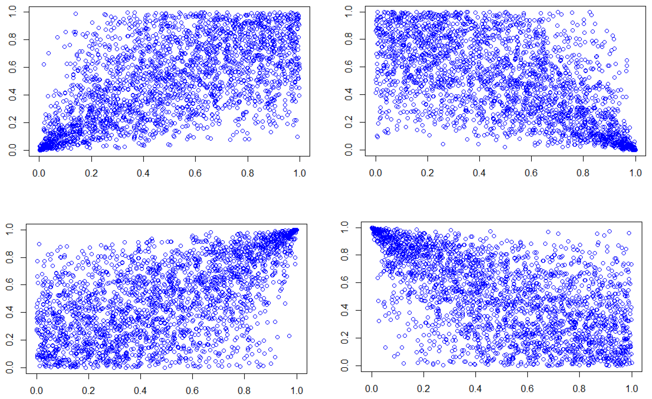
Four scatter plots of simulated data from a non-rotated and rotated Clayton copulas with the parameter
are drawn in
Figure 1. The scatter plots correspond to four different combinations of associations between extreme values, that is, low–low (top left), high–low (top right), high–high (bottom left) and low–high (bottom right).
Once the copula function has been selected, it can be estimated using maximum likelihood estimation or other estimation techniques. The fitted copula function can then be used to make predictions about future combinations of rainfall and temperature values, as well as to estimate the probability of extreme events, such as droughts or heatwaves.
2.3. Data
We analyzed the data on rainfall and temperature for the municipality of Agerola (in the province of Naples; Italy), which us characterized by an altitude of 620 m. The data are recorded with a daily frequency by the Centro Funzionale Multirischi of the Protezione Civile in Campania (Italy), and are publicly available.
The number of weather stations, their location, and other useful information can be obtained from the website of Centro Funzionale Multirischi (
http://centrofunzionale.regione.campania.it/ accessed on 7 June 2023), which is, however, in the Italian language. The location of the station in Agerola can be seen in
Figure 2.
We have analyzed the daily frequency in the period 2008–2022 for a total of 5477 observations.
The variables are:
₋ Rainfall (in mm);
₋ Maximum temperature (in Celsius);
₋ Minimum temperature (in Celsius);
₋ Median temperature (in Celsius).
From the Pearson correlation matrix in
Table 1 it is clear that the three variables measuring the temperature are highly correlated. For that reason, we focus on one of these: Maximum temperature.
The descriptive statistics for the variables Rainfall and Maximum temperature are reported in
Table 2 and
Table 3. The comparison between median and mean strongly suggests a high positive asymmetry for the distribution of the variable Rainfall, which is characterized by more than half of the observations being equal to 0. The variable Maximum temperature exbihits a substantial symmetry.
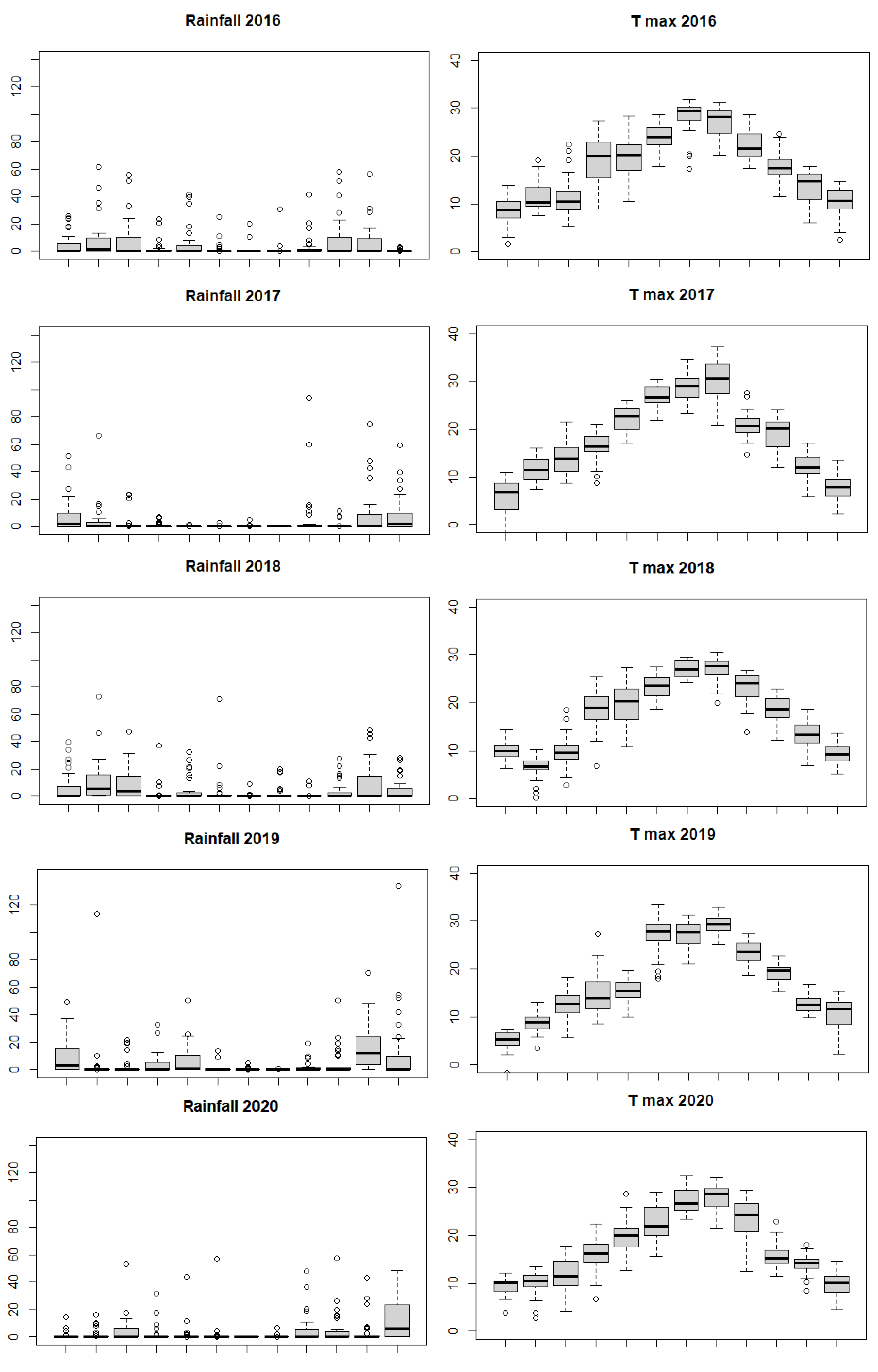
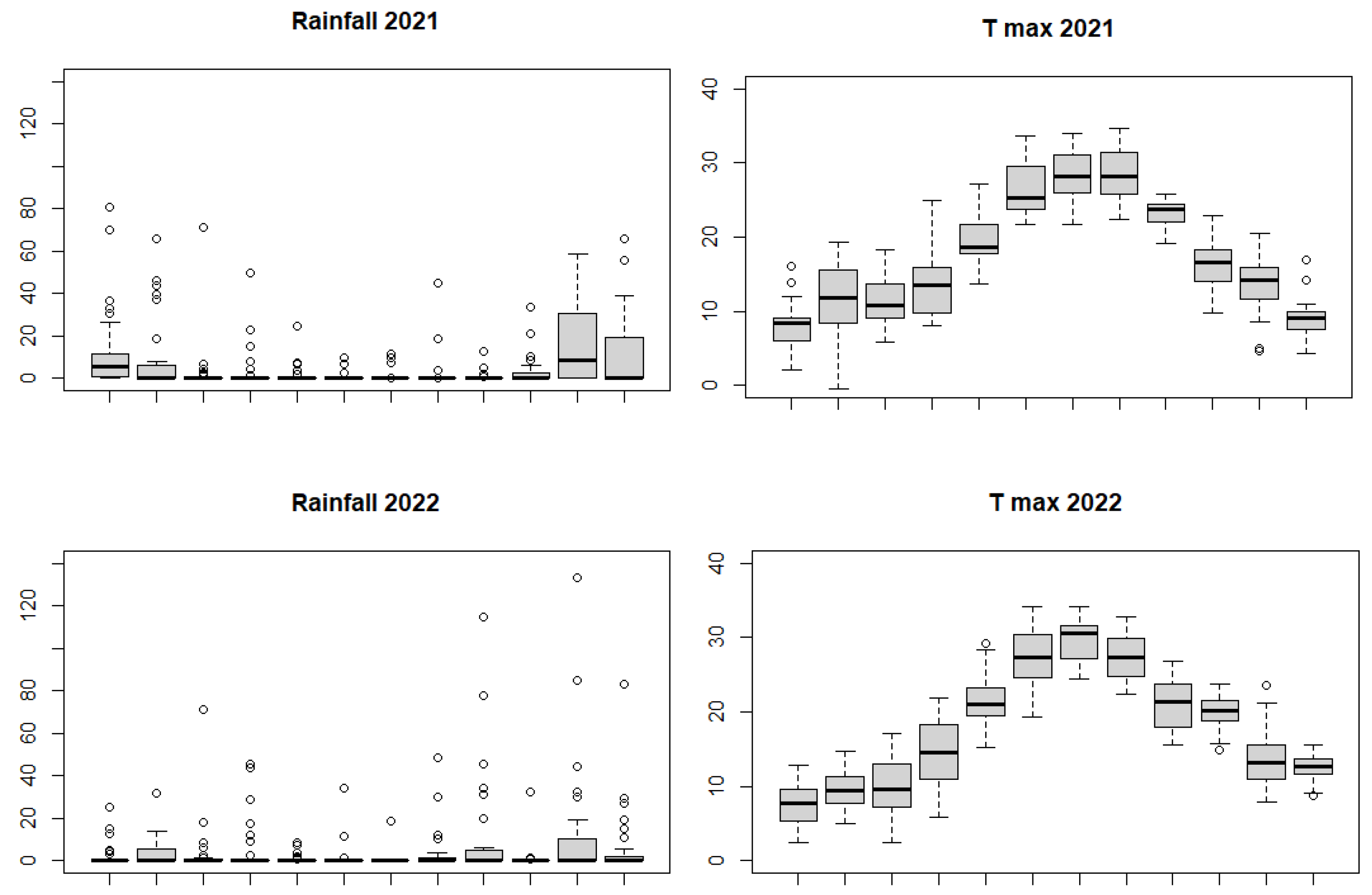
Figure 3 shows box-plots for the two variables in the even years from 2008 to 2022, month-by-month. The circles are observations outside of the whiskers of the box-plot, that is, observations lower than
or larger than
, where
and
denote, respectively, the first and third quartile, while
is the interquartile range. In practice these observations are potentially outliers. Keeping the same scale on the y-axis, we note in the most recent year (2022) the high number of outliers and their size which are definitively larger. In 2022 we observe six observations over 60 mm, and two of them over 100, which is never observed in the previous years.
3. Results and Discussion
This study aims to derive a bivariate model for daily temperature and daily rainfall processes which can be used to simulate and predict temperature and rainfall variations where the dependence structure is measured using copula. The relevant issue is to find a good model for the dependence structure, which is able to capture the tail(s) dependence(s).
Our bivariate model is derived by coupling the marginals of temperature and rainfall distribution to a joint probability distribution for temperature and rainfall processes.
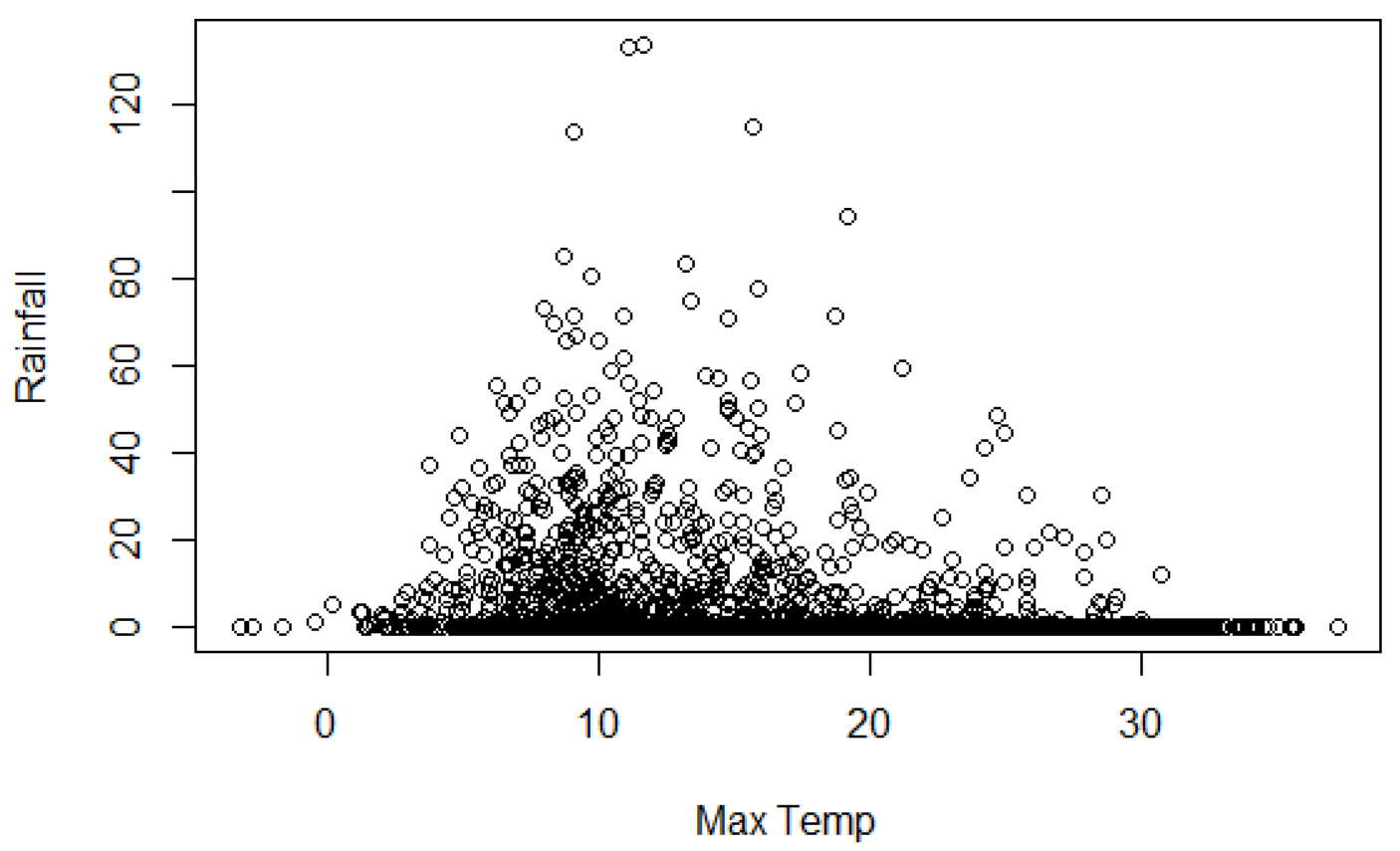
The scatter plot between Maximum temperature and Rainfall (
Figure 4) suggest a negative relationship, which is confirmed by the correlation coefficient, which is equal to −0.259 and significantly different from zero (the
p-value is approximately null). However, before defining a statistical model, we filter the two series for possible autocorrelation and/or seasonality.
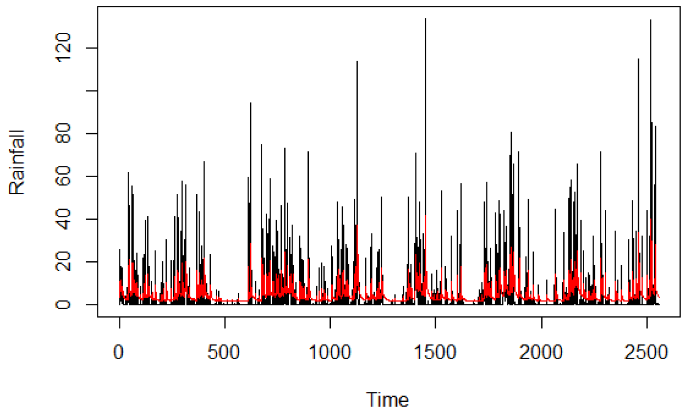
The filtering model for the variable Rainfall (
) is the ARMA(2,1) model which minimizes the AIC, taking into account that negative values are not allowed
The estimates are reported in
Table 4. The
p-values of the Ljung–Box statistics with m = 1, 5, 10, 20, 30 are, respectively, 0.87, 0.09, 0.20, 0.07, 0.14. In
Figure 5 we report the original time series and the fitted values.
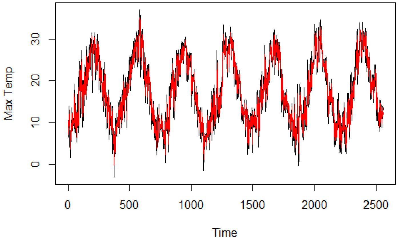
For the variable Maximum temperature (
), we have identified the ARMA(2,2) model,
The estimates are reported in
Table 5. The
p-values of the Ljung–Box statistics with m = 1, 5, 10, 20, 30 are, respectively, 0.97, 0.99, 0.99, 0.99, 0.76. In
Figure 6 we report the original time series and the fitted values.
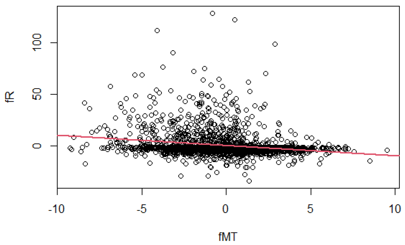
The bivariate modelling is estimated between the two filtered time series (the residuals of the two models), representing the unpredictable components of Rainfall and Maximum temperature, denoted by
and
. In
Figure 7 we show a scatter plot of the filtered variables and the estimated regression line with a significant negative slope (the
p-value is approxiamtely null).
However, to have a joint distribution function that takes into account extreme values, we use a copula function, , where denotes the distribution function of Rainfall and denotes the distribution function of Maximum temperature. The selection of the copula function is limited to the copulas allowing for a negative dependence. There were 10 candidate copulas: Gaussian, Student’s t, rotated (90 and 270 degress) Clayton, rotated (90 and 270 degress) Gumbel, rotated (90 and 270 degress) BB1 and rotated (90 and 270 degress) BB7 copula. Both Gaussian and Student’s t copulas belong to the so-called family of elliptical copulas and are characterized by the correlation coefficient . The Clayton, Gumbel, BB1, and BB7 copulas are Archimedean copulas which only admit positive dependence in the original formulation, and for this reason, are estimated in the rotated extensions allowing for negative dependence.
The estimated distribution functions of the two variables are obtained as empirical distribution functions, and .
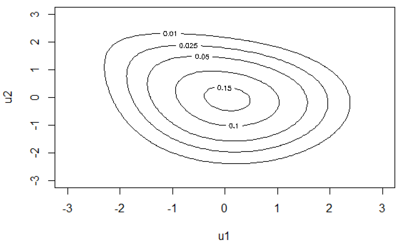
The AIC criterion suggests the rotated 270 degress Clayton copula with the
parameter and a standard error equal to 0.028, which involves the parameter
being highly significant (see
Table 6). As a result,
(with a
p-value less than 0.01). Moreover, the rotated 270 degress Clayton copula with
implies the following tail dependence coefficient:
and
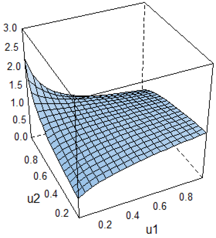
. Finally, the contour plot of the estimated copula is reported in
Figure 8, while the bivariate copula density can be visualized in
Figure 9.
To show the possible use of the results, we have simulated
M values for
for some specific values of
. We have assumed that
.
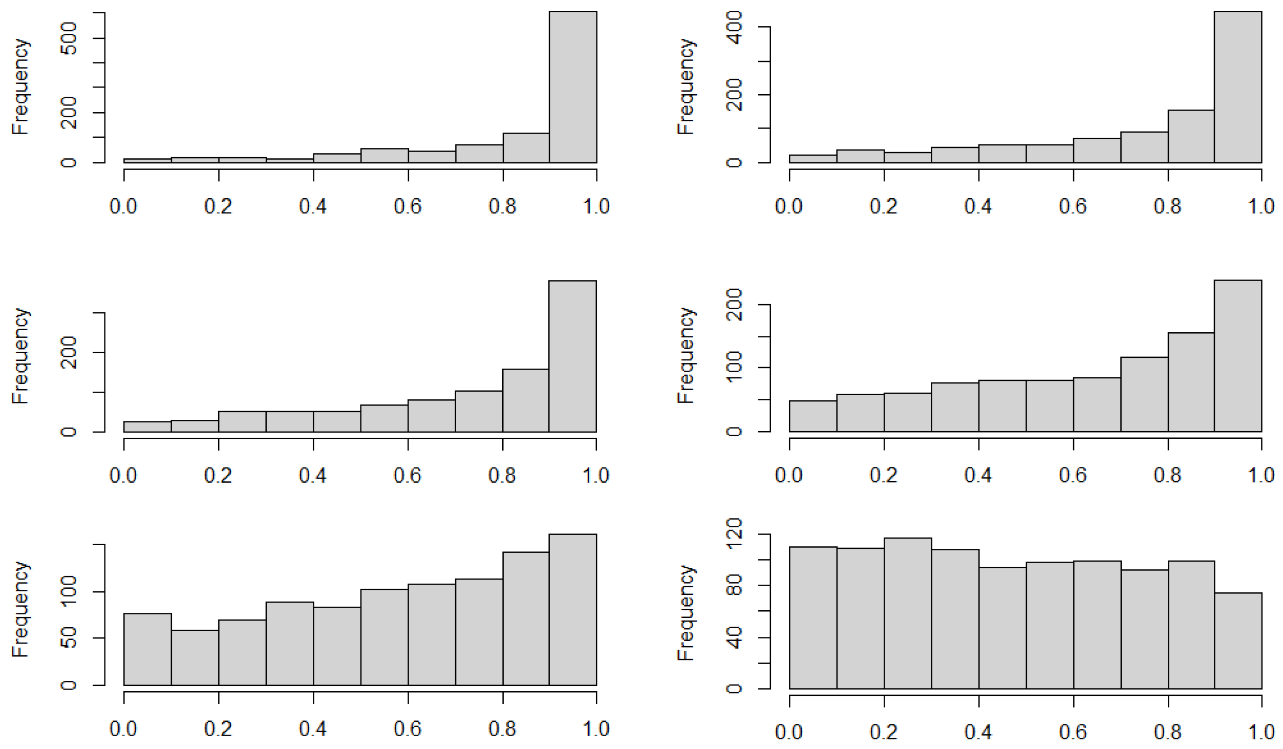
Figure 10 reports six histograms for the simulated values with
M = 1000. In the top-left and top-right panels, we drew the histograms for the
M simulated values of
when the variable Maximum temperature has assumed an extremely low value (the 0.1th percentile, that is
, at the left and 0.5th percentile that is
, at the right). Given that the estimated rotated 270 degrees Clayton copula show
, we find a peak in correspondence with low values of
, that is in correspondence with low percentiles of Maximum temperature. The middle-left and middle-right panels report histograms for when
and
, showing the occurrence of high percentiles of values in the top decile of Rainfall, though this feature is less pronounced for
Finally, in the two histograms in the bottom part of the histogram, the prevalence of the high values of Rainfall reduces; in particular, when
. When we consider the median value of the Maximum temperature, the histogram is approximately uniform; therefore, there is no dependence with the percentile of Rainfall.
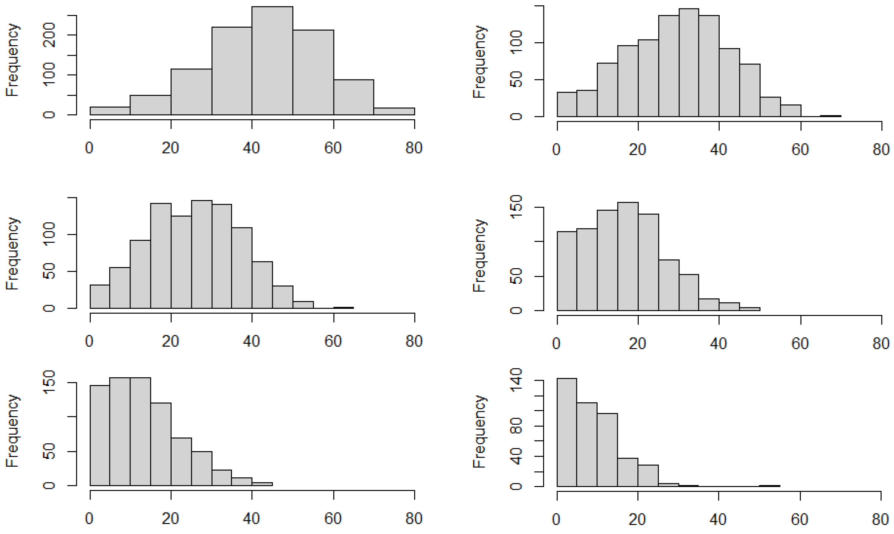
From a practical point of view, one can be interested in the simulated values of the variable Rainfall. This implies that we can “translate” the simulated percentiles into values for Rainfall. To this end, we have to simulate from the statistical model that we have estimated for the variable Rainfall, ARMA(2,1). First, we transform the simulated percentiles of the filtered series (residual) into residuals, using the inverse normal function. Then, we simulate
M values from the statistical model ARMA(2,1) with innovations given by the generated residuals. Finally, we build the histograms (
Figure 11) for the positive values to show the results, discarding the negative values provided by the simulation. It is evident that the smaller the percentile of the simulation, the further to the right the distribution of the generated values for Rainfall. In particular, we can observe that very high values around 80 can be reached only starting from the lowest percentile of
and that the peak around zero is observed starting from the highest percentile (50th) of
.
These examples show the high flexibility of the copula tool which allows us to plan many different simulation studies to take under control a variety of different situations.


