Article

An Extended Flood Characteristic Simulation Considering Natural Dependency Structures

1
Faculty of Civil Engineering, Baden-Württemberg Cooperative State University Mosbach, 74821 Mosbach, Germany
2
Institute for Hydraulic Engineering and Technical Hydromechanics, TUD Dresden University of Technology, 01219 Dresden, Germany
3
Department of Hydraulic Engineering and Hydromechanics, Bochum University of Applied Sciences, 44081 Bochum, Germany
*
Author to whom correspondence should be addressed.
Hydrology 2023, 10(12), 233; https://doi.org/10.3390/hydrology10120233
Submission received: 30 October 2023 / Revised: 20 November 2023 / Accepted: 4 December 2023 / Published: 6 December 2023

Abstract

:
The design of a river-basin-specific flood hydrograph generator based on gauge records enables the generation of synthetic flood hydrographs for the dimensioning of hydraulic structures. Based on selected flow time series, flood waves can be described using four parameters based on flood characteristic simulations, as described by Leichtfuss and Lohr (1999). After successfully adapting suitable distribution functions, dependencies in the load structure are quantified in the next step using copula functions. This newly developed approach builds on the procedure proposed by Bender and Jensen (2012), which assumes hydrological independence. Using copula functions results in increased accuracy in the extended flood characteristic simulation. Moreover, considerable enhancements are achieved through the utilization of genetic algorithms, wherein the descending branch of the flood hydrograph is adjusted by employing an additional variable factor. Subsequently, any number of synthetic flood hydrographs can be generated by combining these parameters. In keeping with the principle of Monte Carlo simulation, a sufficiently high number of synthetic events results in extreme conditions with a low probability of occurrence being reliably represented. Hence, this endeavor has the potential to enhance result reproducibility and prediction quality. As a result, this expanded approach can be employed to provide dependable assessments regarding inflows aimed at optimizing reservoir capacity, for instance.

1. Introduction

Extreme flood hydrographs are frequently used in water management and hydraulic engineering due to their importance. In the design of hydraulic structures, it is often not sufficient to rely only on peak discharges; naturally, additional factors need to be considered. It is therefore crucial to consider the volume associated with the particular design of a hydrograph. In Germany, for example, the relevant regulations require that both flood peaks and volumes are taken into account for the design of dams [1]. This is mandatory because they provide more accurate information about the inflows that maximize the capacity of the reservoir. It should be noted here that these extreme flood hydrographs are usually derived from synthetic design events, which are rarely observed in practice. Still, synthetic hydrographs offer advantages beyond reservoir design, as they can be used for sizing drainage structures and pumping stations or as input to unsteady flow models, particularly for levee systems.
Currently, there are several methods available for describing synthetic hydrograph shapes. Starting with a description using a triangular shape, the mapping of synthetic hydrographs has been continuously developed and refined [2]. However, these methods are subject to certain limitations or require a large database of information. For instance, the approach proposed by Fouroud and Broughton [3] and Bhuyan et al. [4] is often of minor use due to the catchment area size.
Additionally, several other issues such as precipitation data, knowledge about the catchment area, geomorphological aspects, numerical and statistical analyses of peak flows based on observed values, and the utilization of digital terrain models need to be kept in mind and should be considered additional sources of information [3,4,5,6,7,8,9,10,11]. Table 1 provides an exemplary overview characterizing the aforementioned input parameters for determining a flood hydrograph in each respective method. Additionally, there are further statistical methodologies, such as those used to simulate coastal storm surge events, that are not discussed in the present study [12,13].
Hence, building upon the approach established by Leichtfuss and Lohr, which is similarly employed, for instance, in the “Determination of design discharges according to DIN 19700 in North Rhine-Westphalia” guideline issued by the MUNLV (the Ministry of Environment, Agriculture, and Consumer Protection of the state of North-Rhine Westphalia, Germany), an alternative method has been introduced as a substitute for conventionally intricate precipitation-runoff modeling [5,14,15]. This method aims to generate synthetic design hydrographs based only on observed flow time series. With sufficient data availability in the form of flow time series, this approach can be applied to any application area, regardless of the catchment size. Given that the application to a case study revealed shortcomings in the method’s ability to accurately represent prolonged peak discharges in a natural manner, Bender and Jensen formulated an enhanced approach [5]. This revised approach effectively addresses this weakness of the methodology.
The main objective of this research is to highlight the prevailing shortcomings of both approaches and improve simulation results accordingly. In order to achieve this objective, copula functions and genetic algorithms are employed. The fundamental questions are as follows: How can synthetic scenarios be generated effectively considering the hydrological boundary conditions? And what is the impact of applying genetic algorithms to the mathematical representation of the descending branch?

2. Extended Flood Characteristic Simulation according to Bender and Jensen

The primary flood characteristic simulation methodology proposed by Leichtfuss and Lohr is based on a four-parameter approach, which involves describing the temporal evolution of a flood event using parameters, including the rising duration, tr; the shape parameter of the rising branch, sr; the peak discharge, QP; and the shape parameter of the descending branch, sd. Synthetic hydrographs are then generated based on these parameters [14].
However, the enhanced approach introduced by Bender and Jensen further improves flood characteristic simulations by incorporating an additional parameter, namely, the peak duration, tP. The shape parameters sr and sd are dimensionless input parameters used in the hydrograph function and describe the characteristics of the rising and falling branches of the flood wave, respectively. The interaction between all these parameters (rising duration, tr; the shape parameter of the rising branch, sr; peak discharge, QP; peak duration, tp; and the shape parameter of the descending branch, sd) and the resulting shape of the hydrograph is illustrated in Figure 1 [5].

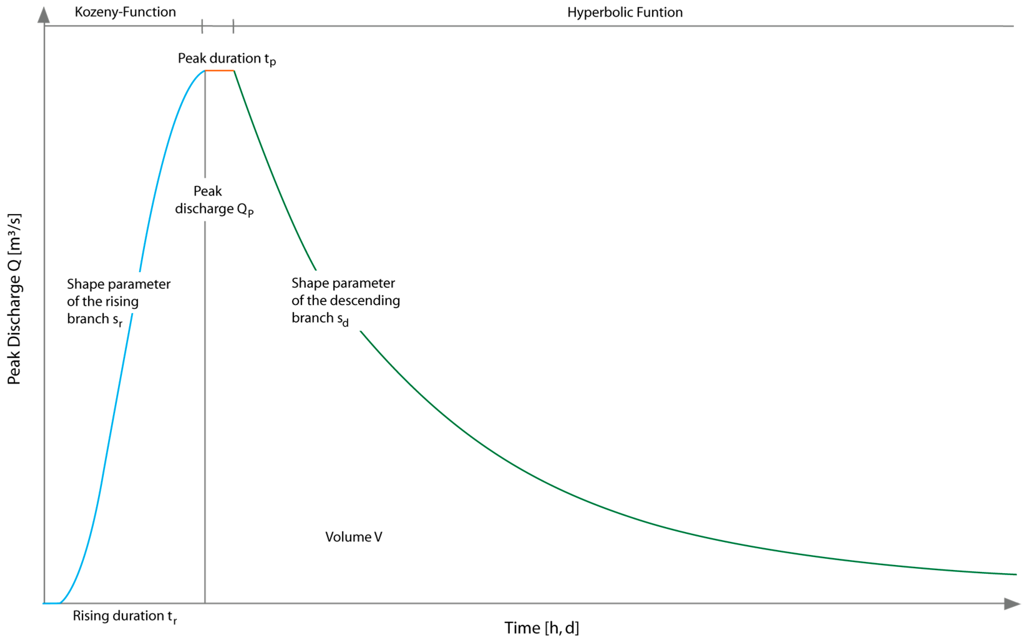
2.1. Hydrograph Functions

Within the flood characteristic simulation, the mathematical portrayal of the hydrograph entails a differentiation between the rising and descending branches of the hydrograph. These components are parameterized using distinct and independent functions and are represented in Equations (1)–(4), as outlined below. The rising branch is modeled using the Kozeny function, while the descending branch follows a hyperbolic function [16,17].
In these equations, t represents time, t r indicates the duration of the rising branch, Q t describes the total discharge at a given time, and Q B t represents the base discharge at the same time. S r and s d are both shape parameters of the rising and descending branches and are valid between 2 and 10, as well as 0.05 and 4. T S determines the starting point of the descending branch, b is the axis section, and c is the compression factor with a constant of one (1). Q 0 represents the maximum discharge, and Q P represents the peak discharge of the event.
Q t = Q P Q B t × [ ( t t r ) s r × e s r × 1 t t r ] + Q B ( t )
Q D t = Q 0 × 1 ( e k ) c ( e k ) c ( e k ) c + ( e k ) c
k = t s + t [ b + s d × ( t s + t ) ]
t s = 1 2 ln 2 × Q 0 Q P 1 s d
The equation incorporates the peak discharge (QP) and shape parameters (sr and sd) as the primary parameters. The other input variables remain nearly constant and are fixed values. The maximum discharge, which needs to be determined at the beginning of the parameter estimation process, is purely a calculated quantity. A standard value of Q0 = 2 × Q P ( H H Q ) is often used as an example [15]. The term “HHQ” refers to the highest known value, which signifies the maximum recorded value for the particular flow time series used.
The peak duration (tP) generally forms a slightly decreasing or increasing plateau. Consequently, the applied method records all values lower than 0.5% below the flood peak (QP). In cases where a stagnant peak discharge is not observed, a peak duration of tP = 0 is assigned [5].
Based on the existing equations for calculating the respective discharge value, the total volume (Vtot) can be calculated using integrals. In this context, it is necessary to distinguish between the rising branch (Vr, as modeled using the Kozeny function) and the descending branch (Vd, as represented using a hyperbolic function). The volume calculation at the peak can be calculated relatively easily with V P = Q P × t P .
Equation (5) describes the calculation of the total volume (from time t = 0 to the last point of the hydrograph, tend), subdivided into its components, for the respective hydrograph.
V t o t = Q P × 0 t r ( t t r ) s r × e ( 1 t t r ) × s r d t + Q P × t P + Q 0 × t S t e n d 1 e k c e k c e k c + e k c d t

2.2. Parameter Identification and Creation of a Synthetic Hydrograph

In parameterization, flow time series are analyzed for flood events with a peak flow (QP) exceeding a certain threshold. According to Leichtfuss and Lohr, a reasonable threshold for parameterization is Q P 2 × Q M [14]. As the current study aims to generate extremely rare synthetic hydrographs with a low probability of occurrence, the principle of the annual maximum series (AMS or AMAX) is used to parameterize the hydrographs [18]. Additionally, it is possible to use critical water levels for river levee dimensioning as a threshold for parameterization.
It is important for accurate parameter determination to ensure that the analyzed flood events are hydrologically independent. This ensures that any flood event influenced by a previous event will not affect the representativeness of the watershed in terms of its shape and peak characteristics [19]. The process for generating synthetic design hydrographs can be summarized as follows:
Initially, a suitable gauge dataset with sufficient information is selected. Then, all parameters are determined based on the principle of the annual maximum series, following the guidelines outlined in Section 2.1. Following this approach guarantees that the sample size remains consistent for each parameter. Appropriate distribution functions are then assigned to these parameter samples (tr, sr, QP, tp, and sd). Upon successful fitting, a large number of synthetic hydrographs can be generated by using the principle of Monte Carlo simulation [20]. Including a sufficient number of synthetic events ensures a desired design event (e.g., HQ10000) among the generated hydrographs. The probability of occurrence of the synthetic hydrographs is directly related to the probability of occurrence of the flood peak (QP).

2.3. Constraints and Enhancement Strategies for the Methodology

The presented procedure was applied to the observed gauge data in Bavaria, Southern Germany (e.g., River Middle Aurach, Emskirchen), spanning the years 1967–2022. This region exhibits diverse hydroclimatic characteristics, encompassing the alpine region in the south, uplands in the north and east, and flatlands in the central and western parts of the area. Furthermore, the methodology was employed in the analysis of the subsequent gauge datasets: the Deggendorf (Kollbach) and Rappoldshofen (Aisch) gauges.
During the implementation, certain deficiencies in the extended flood coefficient simulation became evident. These limitations arose from the aspects described below.

2.3.1. Limitations in Modifying the Descending Branch of the Hydrograph

The previous approach utilized two independent functions—functions (1) and (2)—to assess the fit of the rising and descending branches. The shape parameters of both the rising and descending branches were employed to achieve a high degree of conformity with the observed hydrographs. The goodness of fit between the observed and simulated hydrographs could be assessed, for instance, by utilizing the root-mean-square error (RMSE) [21,22]. Nevertheless, it was found that certain hydrographs exhibited deficiencies in modifying the descending branch. This tendency resulted in an underestimation of the observed hydrograph. Therefore, the current approach introduces an additional parameter, the compression factor, c, which influences the shape of the descending branch and was previously held constant. These parameters (sr, sd, and c) are now determined using an iterative, generation-based optimization method.
  • Genetic algorithm
The genetic algorithm runs through multiple iterations to approach an optimal solution, with each iteration representing a generation. Each generation consists of a population of solution approaches. To enhance the solution routes, the best solutions are combined to form a new generation. The selection of the best routes is based on a fitness score, which, in this case, reflects the deviation between observed and simulated runoff.
The process (Figure 2) begins with an initial generation where solution possibilities are randomly generated for the rising (sr) and descending branches (sd and c). Each member is assigned a route with scores in any order. Elite selection identifies members with the highest fitness and forms the elite pool. From this pool, parents are chosen for the new generation, and each child inherits part of its solution from one parent while filling in the missing part from the other. The population is replenished, and the cycle of fitness calculation and reproduction is repeated over multiple generations. With each generation, the deviation between observed and simulated values diminishes.
Progress eventually reaches a stagnation point when the best possible solution is achieved [23,24].

2.3.2. Seasonal Statistics

In widely used flood statistics, annual maximum flows are commonly used to calculate design variables and quantiles. However, these flows comprise winter and summer events, each with their distinct genesis. In the northern hemisphere, the available data are further divided into the hydrological winter (November–April) and summer periods (May–October).
Various options exist to classify observed floods into different event types. These classifications can be based on factors such as snowmelt from snow cover, catchment characteristics, flood-triggering rainfall amounts, or rainfall durations, among others [11,25]. Deriving such indicators requires data beyond just the runoff series, such as snow depths or precipitation data with a sufficient temporal resolution. However, obtaining such additional data is often not feasible, leading to the subdivision of events into summer and winter categories in the present studies.
For more details on different type-based approaches, one can refer to the given studies in [26,27]. These sources provide additional possibilities for considering different event classifications.

2.3.3. Assumption of Statistical Independence for Individual Parameters

So far, the parameters (tr, sr, QP, tp, and sd) in the collected data have been assumed to be statistically independent of each other [14]. Further investigations should determine the extent to which adjusting the parameters is beneficial for the Monte Carlo simulation. Consequently, the correlation among all existing parameters, including the newly adapted compression factor, c, was subsequently assessed.
  • Correlation
To determine the presence of dependencies between descriptive parameters, the correlation between random variables can be assessed using two statistical measures: linear correlation (Pearson’s r) and rank correlation (Kendall’s τ). Both measures range from minus one to one (−1 to 1), with a value of one (1) indicating complete positive dependence and a value of minus one (−1) indicating complete negative dependence [28,29].
Consequently, the dependencies for the Emskirchen gauge (Middle Aurach) are described using Kendall’s τ (Figure 3). The left side shows the correlation matrix for the summer period, while the right side shows the winter period correlation matrix. Although the resulting values are comparable, they exhibit variations in some parameters. This discrepancy arises from the distinct genesis of the flood hydrographs, as explained in Section 2.3.2, and it describes the respective dependency measure between the measured values.
Nonetheless, both matrices reveal correlations of varying magnitudes, which were considered in the previously valid procedure. This limitation can be addressed by incorporating copula functions.
  • Copula functions
Copula functions are mathematical tools used to model the dependence structure between correlated random variables, independent of their marginal distributions. In the case of n-dimensional variables, copulas are defined as follows:
C : [ 0,1 ] n [ 0,1 ]
Sklar’s theorem establishes the relationship between a copula function and an n-dimensional multivariate distribution as follows [30]:
F X 1 , X 2 , , X n x 1 , x 2 , , x n = C F X 1 x 1 , F X 2 x 2 , , F X n x n
To apply copulas, the marginal distributions of the variables (tr, sr, QS, tp, sd, and c) are first fitted independently to each sample using univariate statistical methods [31]. The observed pairs of variables (X and Y) are subjected to a transformation process that maps them into a range between zero and one. This transformation is achieved by directly applying the obtained distribution functions to the observed values. The corresponding copula model is fitted to these transformed values. Parameter estimation in common copula models often employs Kendall’s τ [32].
For hydraulic and hydrological applications, Archimedean copulas are commonly recommended [13,33]. These single-parameter copula functions are characterized by the parameter θ and can represent a wide range of dependency structures. Commonly employed one-parameter copulas include Clayton, Frank, Joe, and Gumbel copulas [34,35,36,37,38]. Further information on the copulas listed and their generator functions, the value ranges of the copula parameter θ, and the functional relationship between θ and Kendall’s τ can be found, for example, in the following studies [13,31,39].
The selection of appropriate marginal distributions can be determined using the methods described by, e.g., Naghettini [31]. Additionally, the goodness of fit of the copula model should be assessed. Various methods similar to those used for assessing univariate distributions can be employed. Simple measures, including RMSE, between the empirical and parametric copulas, as well as information criteria, such as the Akaike information criterion (AIC) or the Bayesian information criterion (BIC) considering the model parameters, can be used. Further possibilities are also provided by bootstrapping procedures comparing the parametric and non-parametric estimations of copulas based on common tests, such as the Kolmogorov–Smirnov and Cramér von Mises tests [40,41]. It is important to note that the model selected, based on formal fitting tests, may not necessarily be the most hydrologically meaningful. Therefore, hydrological considerations should complement fitting tests. A visual assessment of the overall goodness of fit is also recommended [38].
In addition to analyzing bivariate correlations, it is possible to consider multivariate aspects (e.g., Vines) in which an unlimited number of characteristics can be examined theoretically. Vines are graphical structures that generalize dependency trees and represent joint distributions [42,43,44]. The fundamental concept behind vine copulas involves the creation of high-dimensional copulas through a systematic blending of (conditional) bivariate copulas.
There exist diverse types of Vines [32]. In our scenario, we sequentially investigate dependencies, examining the relationship between the first and second elements, the second and third elements, and so forth. Figure 4 provides a visual representation of building a 3D vine copula with parameters X1, X2, and X3, where their pairwise dependencies are captured through the bivariate copulas C X 1,2 and C X 2,3 . Mathematical mapping is illustrated in the figure [45].

2.3.4. Multi-Peak Flood Events and Uncertainties

In keeping with Bender and Jensen, the methodology employed in this study is applicable to the generation of single-peaked flood hydrographs only [5]. It does not account for the modeling of hydrographs with multiple peaks. The challenge of modeling such complex hydrographs has already been addressed by Klein. By using multivariate statistics, Klein developed a method that enables the superposition of multiple Kozeny functions [45]. In addition, Fischer and Schumann also considered multiple-peaked flood events. In this work, the probability density function of a mixture distribution was used to account for multiple-peaked events for the generation of synthetic design floods [11].
Furthermore, the potential impacts of climate change and its uncertainties are not directly integrated into the methodology. This is because the procedure relies on observed flow time series and, consequently, cannot categorically eliminate uncertainties such as measurement errors. For a more in-depth exploration, we refer the reader to additional literature [46,47].

3. Results

The results focus on two main aspects. Initially, the outcomes of the genetic algorithm, specifically highlighting the enhancements in the goodness of fit of the descending branch achieved through variable combinations of sd and c. Furthermore, the findings derived from the examination of hydrological dependencies within the data and their impact on the results of the extended flood characteristic simulation are discussed in detail. Both adjustments are based on a direct comparison of the simulation accuracy using the detected flood events from the Emskirchen gauge (Middle Aurach).

3.1. Consideration of Combined Genetic Algorithms in Adapting the Descending Branch

Through the utilization of combined (sd and c) genetic algorithms, a greater level of fitting accuracy can be attained in the descending branch, as compared to the previously suggested method by Bender and Jensen, wherein solely the shape parameter is fitted (Figure 5). This improvement is demonstrated through a correlation analysis using Kendall’s (τ) method and the Kling–Gupta efficiency (KGE) metric [29,48]. Here, the observed and simulated flood volumes are considered. In Figure 5, both the observed and simulated flood hydrographs are displayed, depicting the peak discharge (QP) and volume (V).
In the upper section, the genetically adjusted shape parameter for the descending branch remains constant with a compression factor of cfix = 1. In contrast, the lower section shows a variable adjustment of the shape parameter and compression factor, cvar, for the hyperbolic function of the descending branch. For both winter and summer events, a clear improvement in the simulated flood volumes becomes evident due to the variable compression factor. For example, KGE for summer events improves from 0.666 with compression factor cfix = 1 to 0.814 with a variable compression factor. The correlation also improves from 0.89 to 0.951.
Figure 6 illustrates the distinctions in the trajectory of the descending branch, depending on the chosen methodology for the compression factor, using an exemplary flood hydrograph. This highlights the observed flood hydrograph (gray) and the simulated hydrographs with sd and cfix (green), as well as sd and cvar (orange). By utilizing a variable compression factor cvar  ( 0 c 1 ) and sd, there is an improvement in the adaptation of the descending branch to the observed flood hydrograph. This can be justified by acknowledging that both variables have a direct impact on the outcome of the hyperbolic function. With cfix, it is not always possible to achieve a complete correction solely through adjustments of the shape parameter (sd) for certain hydrographs. Thus, the fixed adjustment (cfix) in the example below tends to slightly overestimate the hydrograph in the descending branch.
Figure 7 illustrates a simplified depiction of the procedure for refining the coefficient of variation (cvar) within the range of 0.1 to 1 with two constant shape parameters for the descending branch (sd = 0.05 and 0.40).
It is worth emphasizing that increasing the bandwidth of sd can also encompass a significantly broader spectrum of hydrographs. In contrast, this improvement can not only be corrected in the same way via the variable adjustment of the compression factor but can also be amplified. Consequently, it is possible to not only ascertain the extent of the descending branch within a specified period but also facilitate significant stretching of the originally compressed shape, exerting a substantial influence on the rate of the descent of the descending branch. The simultaneous application of both variables leads to an improvement, as exemplified in Figure 5.

3.2. Consideration of the Dependency Structure between Correlated Random Variables in Terms of Copulas

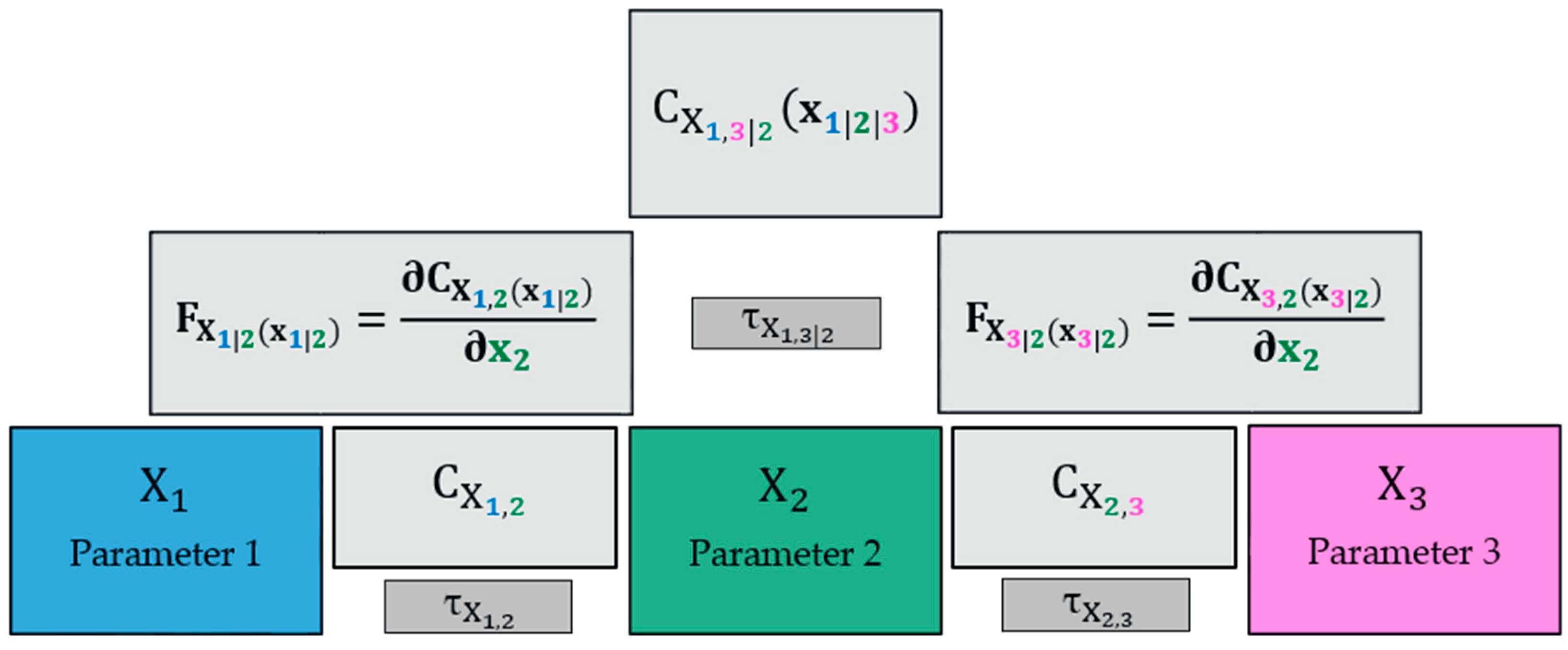
3.2.1. Utilizing D Vines for the Present Application

In the current application, a six-dimensional copula can be constructed as an example according to the concept of Vines based on the correlational parameters (tr, sr, QP, tp, sd, and c) for the winter period [49]. The detailed structure, including the appropriate copulas, is further described by using the subsequent visualization (Figure 8).
To this end, the parameters were tailored using univariate distribution functions. In the current scenario, the GEV, normal, and Weibull distributions were chosen due to their goodness of fit based on the Kolmogorov–Smirnov test [40].
Considering the dependency structure between the correlated random variables in terms of copulas results in a new sample. Adhering to the principles of Monte Carlo simulation, a sufficiently large number of synthetic events can be generated as per Leichtfuss and Lohr [14,20].

3.2.2. Plausibility Check

The enhancement in the proposed approach can be assessed by comparing the replication accuracy based on detected flood events recorded via tide gauges. This involves a comparison between the observed volume and the synthetically simulated values (n = 1000) obtained from both the existing flood characteristic simulation (EFCS) approach without considering natural dependencies and the newly developed enhanced flood characteristic simulation with the copula (EFCSC) approach. A preliminary assessment of the improved results can be gleaned from Figure 9.
The figure displays the volume and peak discharges derived from the observed data (gray), as well as the volume and peak discharges generated synthetically using the EFCS approach (blue) and the newly developed EFCSC approach (orange). Both simulations are based on the adjustment of six variables using genetic algorithms (Section 3.1). The data are further divided into the summer and winter half-year periods.
It is evident that there is a further improvement in the simulation results for both the summer and winter periods. From a computational standpoint, the improvement in the results in the summer period is reflected in an increase in the correlation coefficient from 0.342 (EFCS) to 0.403 (EFCSC). This represents an improvement of 17.8% in the summer and 6.3% in the winter period.

4. Discussion

The improvement in the approach presented is firstly determined through a direct comparison of the accuracy of reproducing detected flood events from the Emskirchen gauge on the Middle Aurach River. In this process, all observed flood hydrographs are parameterized and synthetically reproduced using the extended flood characteristic simulation (EFCS) by Bender and Jensen, as well as the newly developed extended flood characteristic simulation considering natural dependency structures (EFCSC). Notably, to enhance precision in reproducing dependency structures, copula functions are employed as part of the improvement, along with the integration of genetic algorithms.
An initial impression of the enhanced results can be gained by directly overlaying the relationship between the observed and simulated volume and peak discharges, as depicted in Figure 9. This is expected due to the existence of interdependencies between individual parameters that were previously disregarded. Through the application of copula functions, weak (<0.35), moderate (0.36 to 0.67), and strong correlations (>0.68) can be accounted for [50]. This expanded information promptly leads to improved outcomes. Naturally, the degree of improvement strongly relies on the available data.
An additional improvement by incorporating another parameter (compression factor, c) through the adaption of genetic algorithms is shown in Figure 4. This leads to an enhancement in the goodness of fit for the descending branch (Figure 5). Thus, the volume of the flood hydrograph, for instance, in the dimension of hydraulic structures (e.g., weir or river levees) can be associated with higher reliability by integrating this additional parameter.
In conclusion, the presented modification of the extended flood characteristic simulation considering natural dependency structures represents a valid upgrade of the existing method. Although the approach cannot capture multi-peaked hydrographs, the incorporation of an additional parameter (compression factor, c) allows for a significantly more accurate simulation of single-peaked flood events. Moreover, by employing copula functions, the goodness of fit can be further enhanced based on the data foundation for simulated flood hydrographs.
Thus, with the developed methodology, the mapping accuracy can be further improved through the incorporation of copula functions and an additional parameter. Further, it should be noted that, given sufficient data availability in the form of low time series, this method can be applied to any catchment area independently of additional characteristics, e.g., precipitation data, knowledge about the catchment area, geomorphological aspects, and digital terrain models (refer to Table 1). This constitutes a noteworthy advantage; furthermore, a user’s workload experiences only a marginal increase, even as substantial improvements in results are realized.

Author Contributions

Conceptualization, M.A.Ö.; methodology, M.A.Ö., F.S., J.B. and C.M.; software, M.A.Ö. and F.S.; validation, M.A.Ö., F.S. and J.B.; formal analysis, M.A.Ö. and F.S.; investigation, M.A.Ö. and F.S.; resources, M.A.Ö., F.S. and J.B.; data curation, M.A.Ö. and F.S.; writing—original draft preparation, M.A.Ö.; writing—review and editing, M.A.Ö., F.S., J.B., C.M. and J.S.; visualization, M.A.Ö. and F.S.; supervision, M.A.Ö., F.S., J.B., C.M. and J.S.; project administration, M.A.Ö.; funding acquisition, M.A.Ö., J.B. and J.S. All authors have read and agreed to the published version of the manuscript.

Funding

This research was funded by Baden-Württemberg Cooperative State University Mosbach and the joint publication funds of TU Dresden, including the Carl Gustav Carus Faculty of Medicine and SLUB Dresden, as well as the Open-Access Publication Funding of the DFG.

Data Availability Statement

We are grateful to Bayerisches Landesamt für Umwelt (www.lfu.bayern.de, accessed on 8 August 2023) for providing the discharge data. The manuscript provides all the information needed to replicate the results.

Conflicts of Interest

The authors declare no conflict of interest.

References

  1. DIN 19700-10:2004-07; Dam Plants—Part 10: General Specifications. Beuth Publishing: Berlin, Germany, 2004; pp. 1–28. (In German) [CrossRef]
  2. Chow, T.V.; Maidment, D.R.; Mays, L.W. Applied Hydrology; McGraw-Hill: New York, NY, USA, 1988. [Google Scholar]
  3. Fouroud, N.; Broughton, R.S. Flood Hydrograph Simulation Model. J. Hydrol. 1981, 49, 139–172. [Google Scholar] [CrossRef]
  4. Bhuyan, M.K.; Kumar, S.; Jena, J.; Bhunya, P.K. Flood Hydrograph with Synthetic Unit Hydrograph Routing. Water Resour. Manag. 2015, 29, 5765–5782. [Google Scholar] [CrossRef]
  5. Bender, J.; Jensen, J. Ein erweitertes Verfahren zur Generierung synthetischer Bemessungshochwasserganglinien. Wasserwirtschaft 2012, 3, 35–39. (In German) [Google Scholar] [CrossRef]
  6. Wyncoll, D.; Gouldby, B. Application of a multivariate extreme value approach to system flood risk analysis. HR Wallingford Work. Water 2013, HRPP594, 1–17. [Google Scholar]
  7. Candela, A.; Brigandi, G.; Aronica, G.T. Estimation of synthetic flood design hydrographs using a distributed rainfall-runoff model coupled with a copula-based single storm rainfall generator. Nat. Hazards Earth Syst. Sci. 2014, 14, 1819–1833. [Google Scholar] [CrossRef]
  8. Chatzichristaki, C.; Stefanidis, S.; Stefanidis, P.; Stathis, D. Analysis of the flash floods in Rhodes Island (South Greece) on 22 November 2013. Silva Balc. 2015, 16, 76–86. [Google Scholar]
  9. Aranda, J.A.; Garcia-Bartual, R. Synthetic Hydrographs Generation Downstream of a River Junction Using a Copula Approach for Hydrological Risk Assessment in Large Dams. Water 2018, 10, 570. [Google Scholar] [CrossRef]
  10. Shatnawi, A.; Ibrahim, M. Derivation of flood hydrographs using SCS synthetic unit hydrograph technique for Housha catchment area. Water Supply 2022, 20, 4888–4901. [Google Scholar] [CrossRef]
  11. Fischer, S.; Schumann, D. Generation of type-specific synthetic design flood hydrographs. Hydrol. Sci. J. 2023, 68, 982–997. [Google Scholar] [CrossRef]
  12. MacPherson, L.; Arns, A.; Dangendorf, S.; Vafeididis, A.T.; Jensen, J. A Stochastic Extreme Sea Level Model for the German Baltic Sea Coast. J. Geophys. Res. Ocean. 2019, 124, 2054–2071. [Google Scholar] [CrossRef]
  13. Wahl, T.; Mudersbach, C.; Jensen, J. Assessing the hydrodynamic boundary conditions for risk analyses in coastal areas: A multivariate statistical approach based on Copula functions. Nat. Hazards Earth Syst. Sci. 2012, 12, 495–510. [Google Scholar] [CrossRef]
  14. Leichtfuss, A.; Lohr, H. Die stochastisch-deterministische Generierung extremer Abflusszustände. Schriftenreihe FG Wasserbau Und Wasserwirtsch. Univ. Kaiserslaut. 1999, 9. (In German) [Google Scholar]
  15. Ministry of Environment, Agriculture, and Consumer Protection of the state of North Rhine-Westphalia. Ermittlung von Bemessungsabflüssen nach DIN 19700 in Nordrhein-Westfalen. Merkblätter 2010, 46, 1–53. (In German) [Google Scholar]
  16. Dyck, S. Angewandte Hydrologie, Teile 1 und 2. In VEB Verlag für Bauwesen; VEB Verlag für Bauwesen: Berlin, Germany, 1980. (In German) [Google Scholar]
  17. Lohr, H. Generierung extremer Abflüsse für die Stauanlagenbemessung. Wasser Abfall 2003, 7–8, 20–24. (In German) [Google Scholar] [CrossRef]
  18. DWA-Merkblatt (Gelbdruck). Stochastische und deterministische Wege zur Ermittlung von Hochwasserwahrscheinlichkeit; DWA (Deutsche Vereinigung für Wasserwirtschaft, Abwasser und Abfall e.V.): Hennef, Germany, 2023; pp. 22–25. (In German) [Google Scholar]
  19. Mudersbach, C. Untersuchungen zur Ermittlung von hydrologischen Bemessungsgrößen mit Verfahren der Instationären Extremwertstatistik. Dissertation; Universität Siegen: Siegen, Germany, 2009. (In German) [Google Scholar]
  20. Rubinstein, R.Y.; Kroese, D.P. Simulation and the Monte Carlo Method; John Wiley & Sons, Inc.: Hoboken, NJ, USA, 2008; Volume 707. [Google Scholar] [CrossRef]
  21. Chai, T.; Draxler, R.R. Root mean square error (RMSE) or mean absolute error (MAE)?—Arguments against avoiding RMSE in the literature. Geosci. Model Dev. 2014, 7, 1247–1250. [Google Scholar] [CrossRef]
  22. Hodson, T.O. Root-mean-square error (RMSE) or mean absolute error (MAE): When to use them or not. Geosci. Model Dev. 2022, 15, 5481–5487. [Google Scholar] [CrossRef]
  23. Schöneburg, E.; Heinzmann, F.; Feddersen, S. Genetische Algorithmen und Evolutionsstrategien—Eine Einführung in Theorie und Praxis der simulierten Evolution; Addison-Wesley: Bonn, Germany, 1981; pp. 1–481. ISBN 978-3-89319-493-3. (In German) [Google Scholar]
  24. Tanweer, A.; Shamimul, D.; Amit, D.; Mohamed, B. Genetic Algorithm: Reviews, Implementations, and Applications. Int. J. Eng. Pedagog. 2020, 20, 2–18. [Google Scholar] [CrossRef]
  25. Fischer, S.; Schumann, A. Berücksichtigung von Starkregenereignissen in der saisonalen Hochwasserstatistik mit Hilfe statistischer Mischungsmodelle. HyWa 2017, 61, 36–49. (In German) [Google Scholar] [CrossRef]
  26. Merz, R.; Blöschl, G. Flood frequency regionalization—Spatial proximity vs catchment attributes. J. Hydrol. 2005, 302, 283–306. [Google Scholar] [CrossRef]
  27. Tarasova, L.; Merz, R.; Kiss, A.; Basso, S.; Blöschl, G.; Merz, B.; Viglione, A.; Plötner, S.; Guse, B.; Schumann, A.; et al. Causative classification of river flood events. Wiley Interdiscip. Rev. Water 2019, 6, e1353. [Google Scholar] [CrossRef]
  28. Hartung, J.; Elpelt, B. Multivariate Statistik: Lehr- und Handbuch der angewandten Statistik; De Gruyter Oldenbourg: Berlin, Germany, 2006; Volume 6. (In German) [Google Scholar]
  29. Kendall, M.G. A New Measure of Rank Correlation. Biometrika 1938, 30, 81–93. [Google Scholar] [CrossRef]
  30. Sklar, A. Fonctions de Répartition à n Dimensions et Leurs Marges. In Publications de l’Institut Statistique de l’Université de Paris; l’Institut Statistique de l’Université de Paris: Paris, France, 1958; Volume 8, pp. 229–231. (In French) [Google Scholar]
  31. Naghettini, M. Fundamentals of Statistical Hydrology; Springer: Berlin/Heidelberg, Germany, 2017. [Google Scholar] [CrossRef]
  32. Roger, B.N. An Introduction to Copulas; Springer: New York, NY, USA, 2006; ISBN 978-1441921093. [Google Scholar]
  33. Favre, A.C.; El Adlouni, S.; Perreault, L.; Thiémonge, N.; Bobée, B. Multivariate hydrological frequency analysis using copulas. Water Resour. Res. 2004, 40, 1–12. [Google Scholar] [CrossRef]
  34. Clayton, D.G. A model for association in bivariate life tables and its application in epidemiological studies of familial tendency in chronic disease incidence. Biometrika 1978, 65, 141–151. [Google Scholar] [CrossRef]
  35. Frank, M.J. On the simultaneous associativity of F(x,y) and x + y − F(x,y). Aequ. Math. 1979, 19, 194–266. [Google Scholar] [CrossRef]
  36. Joe, H. Multivariate Models and Dependence Concepts; Chapman and Hall: New York, NY, USA, 1997. [Google Scholar]
  37. Gumbel, E.J. Distributions des valeurs extremes en plusieurs dimensions. In Publications de l’Institut Statistique de l’Université de Paris; l’Institut Statistique de l’Université de Paris: Paris, France, 1960; Volume 9. (In French) [Google Scholar]
  38. Bender, J. Zur Ermittlung von hydrologischen Bemessungsgrößen an Flussmündungen mit Verfahren der multivariaten Statistik. In Mitteilungen des Forschungsinstituts Wasser und Umwelt der Universität Siegen Heft 9; Mitteilungen des Forschungsinstituts Wasser und Umwelt der Universität Siegen: Siegen, Germany, 2015. (In German) [Google Scholar]
  39. DWA-Merkblatt DWA-M520; Probabilistische Methoden im Wasserbau. DWA (Deutsche Vereinigung für Wasserwirtschaft, Abwasser und Abfall e.V.): Hennef, Germany, 2023; pp. 39–42. (In German)
  40. Genest, C.; Favre, A.C. Everything you always wanted to know about copula modelling but were afraid to ask. Water Resour. Res. 2007, 43, W090401. [Google Scholar] [CrossRef]
  41. Salvadori, G.; De Michele, C. On the use of copulas in hydrology: Theory and practice. J. Hydrol. Eng. 2007, 12, 369–380. [Google Scholar] [CrossRef]
  42. Cooke, R.M. Markov and entropy properties of tree and vines—Dependent variables. In Proceedings of the ASA Section of Bayesian Statistical Science; American Statistical Association: Alexandria, VA, USA, 1997. [Google Scholar]
  43. Bedfort, T.J.; Cooke, R.M. Vines—A new graphical model for dependent random variables. Ann. Stat. 2002, 30, 1031–1068. [Google Scholar] [CrossRef]
  44. Lanzafame, R.; Timmermans, M.; Orlins, F.; Valls, S.S.; Napoles, O.M. Probabilistic Design for Civil Engineering Infrastructure Using Vine-Copulas. In Proceedings of the 31st European Safety and Reliability Conference, Angers, France, 19–23 September 2021. [Google Scholar] [CrossRef]
  45. Klein, B. Ermittlung von Ganglinien für die Risikoorientierte Hochwasserbemessung von Talsperren. Ph.D. Thesis, Schriftenreihe Hydrologie/Wasserwirtschaft an der Ruhr-Universität Bochum, Bochum, Germany, 2009. (In German). [Google Scholar]
  46. Quesada-Montano, B.; Di Baldassarre, G.; Rangecroft, S.; Van Loon, A.F. Hydrological change: Towards a consistent approach to assess changes on both floods and droughts. Adv. Water Resour. 2018, 111, 31–35. [Google Scholar] [CrossRef]
  47. Gaur, S.; Bandyopadhyay, A.; Singh, R. Modelling potential impact of climate change and uncertainty on streamflow projections: A case study. J. Water Clim. Chang. 2021, 12, 384–400. [Google Scholar] [CrossRef]
  48. Gupta, H.V.; Kling, H.; Yilmaz, K.K.; Martinez, G.F. Decomposition of the mean squared error and NSE performance criteria: Implications for improving hydrological modelling. J. Hydrol. 2009, 377, 80–91. [Google Scholar] [CrossRef]
  49. Gräler, B.; Van den Berg, M.J.; Vandenberghe, S.; Petroselli, A.; Grimaldi, S.; De Baets, B.; Verhoest, N.E.C. Multivariate return periods in hydrology: A critical and practical review focusing on synthetic design hydrograph estimation. Hydrol. Earth Syst. Sci. 2013, 17, 1281–1296. [Google Scholar] [CrossRef]
  50. Taylor, R. Interpretation of the Correlation Coefficient: A Basic Review. J. Diagn. Med. Sonogr. 1990, 1, 35–39. [Google Scholar] [CrossRef]
Figure 1. Influencing parameters of the hydrograph [5].
Hydrology 10 00233 g001
Figure 2. Example process of genetic algorithms.
Hydrology 10 00233 g002
Figure 3. Correlation matrix for summer (left) and winter (right) periods.
Hydrology 10 00233 g003
Figure 4. Hierarchical nesting of bivariate copulas in the construction of a 3D vine copula including mathematical mapping.
Hydrology 10 00233 g004
Figure 5. Comparison of sd and cfix with sd and cvar using Kendall’s τ and KGE (Middle Aurach, Emskirchen).
Hydrology 10 00233 g005
Figure 6. Example of individually simulated hydrographs compared to the observed hydrograph.
Hydrology 10 00233 g006
Figure 7. Adjustment of cvar to the fitting of the descending branch at a constant sd = 0.05 (left) and 0.40 (right).
Hydrology 10 00233 g007
Figure 8. D Vine structure of the parameters (tr, sr, QP, tp, sd, c) for the summer period of the river Middle Aurach (Emskirchen).
Hydrology 10 00233 g008
Figure 9. Correlation of observed and simulated (EFCS and EFCSC) volume and peak discharges at the Emskirchen (Middle Aurach) gauge.
Hydrology 10 00233 g009
Table 1. Initial data determining the flood hydrograph.
AuthorInitial Parameters
Fouroud and Broughton (1981) [3]
Hydrology 10 00233 i001
    Precipitation data
Bender and Jensen (2012) [5]
Hydrology 10 00233 i002
    Catchment area conditions
Wyncoll and Couldby (2013) [6]
Hydrology 10 00233 i003
    Geomorphological characteristics
Candela et al. (2014) [7]
Hydrology 10 00233 i004
    Land cover data, digital elevation model
Chatzichristaki et al. (2015) [8]
Hydrology 10 00233 i005
    Numerical simulations
Bhuyan et al. (2015) [4]
Hydrology 10 00233 i006
    Statistical analysis based on observation data
Aranda and Garcia-Barthual (2018) [9]
Hydrology 10 00233 i007
Shatnawi and Ibrahim (2022) [10]
Hydrology 10 00233 i008
Fischer and Schumann (2023) [11]
Hydrology 10 00233 i009
Disclaimer/Publisher’s Note: The statements, opinions and data contained in all publications are solely those of the individual author(s) and contributor(s) and not of MDPI and/or the editor(s). MDPI and/or the editor(s) disclaim responsibility for any injury to people or property resulting from any ideas, methods, instructions or products referred to in the content.

