A Soil Moisture Profile Conceptual Framework to Identify Water Availability and Recovery in Green Stormwater Infrastructure

Abstract

The recovery of soil void space through infiltration and evapotranspiration processes within green stormwater infrastructure (GSI) is key to continued hydrologic function. As such, soil void space recovery must be well understood to improve the design and modeling and to provide realistic expectations of GSI performance. A novel conceptual framework of soil moisture behavior was developed to define the soil moisture availability at pre-, during, and post-storm conditions. It uses soil moisture measurements and provides seven critical soil moisture points (A, B, C, D, E, F, F″) that describe the soil–water void space recovery after a storm passes through a GSI. The framework outputs a quantification of a GSI subsurface hydrology, including average soil moisture, the duration of saturation, soil moisture recession, desaturation time, infiltration rates, and evapotranspiration (ET) rates. The outputs the framework provide were compared to the values that were obtained through more traditional measurements of infiltration (through spot field infiltration testing), ET (through a variety of methods to quantify GSI ET), soil moisture measurements (through the soil water characteristics curve), and the duration of saturation/desaturation time (through a simulated runoff test), all which provided a strong justification to the framework. This conceptual framework has several applications, including providing an understanding of a system’s ability to hold water, the post-storm recovery process, GSI unit processes (ET and infiltration), important water contents that define the soil–water relationship (such as field capacity and saturation), and a way to quantify long-term changes in performance all through minimal monitoring with one or more soil moisture sensors. The application of this framework to GSI design promotes a deeper understanding of the subsurface hydrology and site-specific soil conditions, which is a key advancement in the understanding of long-term performance and informing GSI design and maintenance.

1. Introduction

Green stormwater infrastructure (GSI) is an essential tool to reduce the impact of increased runoff due to urbanization. Biofiltration GSI specifically has been widely used for its multifaceted benefits of reducing stormwater runoff via enhancing infiltration and evapotranspiration [1,2,3,4]. Two key aspects of vegetated GSI systems, such as bioinfiltration basins, are how the system fills during a storm event and the subsequent recovery process. The recovery of GSI can be thought of in two steps: 1. how quickly water moves into the underlying soil or underdrain system (the infiltration-dominated phase), and 2. how long it takes for the system to reestablish the water holding capacity within the pond and/or soil void space (the evapotranspiration-dominated phase [3,5]). Analysis of the soil moisture profile from the beginning through to the recovery provides insight into the in situ efficacy of the GSI design and its performance over time. Improved understanding of GSI subsurface hydrology improves the design (e.g., decisions on soil type and depth [6]), validates continuous modeling efforts [7], provides realistic expectations of GSI performance in response to managing storm events, and could be an indicator of needed maintenance. As stormwater management evolves and attention is focused on resilience and cost-effective design, aligning design and maintenance with the observed treatment capabilities of GSI is fundamental to advancing stormwater management practice.

For vegetated GSI, typically an engineered soil mix is used to enhance infiltration, support vegetation to provide evapotranspiration (ET), and provide some temporary storage in void space to manage incoming stormwater runoff. Past studies of ET are generally indicated as a gradual loss of water by weight [3,5,8], where a gradual decrease in the soil moisture was assumed as void space recovery in the GSI due to ET.

For the soil moisture profile curve (increases with water input and slowly decreases as the dry period increases), it is uncertain how the water is being held in the system. This means that the water may either be retained in the soil or percolate quickly and re-capture water from a nearby soil layer; thus, it is difficult to analyze the true moisture in the system. The authors in [5] indicated that there was a distinct change in the slope of the recession limb for deep infiltration compared to evapotranspiration loss. The study also mentions that the change in soil moisture is indicative of the amount of water stored in the soil layer and is available for its removal process (either through ET or infiltration). While the study provided appropriate evapotranspiration loss between the storms, the entire ET loss was discussed based on the total weight loss on a daily scale as the observations analyzed were during dry days after percolation ended.

As water moves down the soil layer, the rate at which it desaturates through the soil layer varies [9] at distinct depths; therefore, the uptake of water by the plants may vary depending on the soil depth and its defined root zone area. Such details regarding the soil and water relationship at the subsurface layer are still not used in subsurface estimation, leaving a gap between the actual and measurable value of the subsurface parameters. This study addresses such challenges by presenting a conceptual framework where changes in soil moisture are defined to analyze the soil subsurface layer.

Several soil moisture-related studies have been conducted that rely on soil moisture profile categorization [4,5,10,11]. These authors briefly discussed the soil moisture trends and how they change due to water availability scenarios. Their studies are based on these trends where they have used hydrological parameters to define soil moisture in their respective soil moisture. Although the moisture trends are deliberated over the hydrological behavior, a strategic framework on how these moisture trends can be quantified is necessary. The purpose of the present research was to provide a quantitative tool, where the user can conceptualize the soil moisture profile to monitor the subsurface layer at varying water availability scenarios.

For a soil moisture profile, ref. [9] used soil moisture sensor data to quantify the desaturation time into soil layers based on the soil moisture measurements at three bioinfiltration systems. The study discussed the systems’ ability to hold water at its maximum soil moisture condition (i.e., at saturation) at each of the distinct soil depths and the time required by the systems to remain saturated at each of these depths. As soil depth increased, the saturation time increased and the movement of water was discussed at the end of the saturation for each of these depths. The study was a preliminary study based on nine rainfall events and indicated that a more robust analysis was needed, which led to the present work.

In the current work, it was observed through soil moisture monitoring in GSI that a consistent and repeatable structure of soil moisture profile occurs in response to a storm event. This response was based on 58 storm events. As demonstrated in Figure 1, first the soil moisture has a rapid increase as the rainfall-to-runoff moves into the system and then plateaus as it reaches saturation (during saturating storm event). After the storm event, the soil moisture decreases quickly as water exits to the underlying surface (primarily via infiltration) or sewer system (via underdrain) and then very slowly over time (primarily through ET; Figure 1).

Focusing on the soil moisture profile over time enables a quantitative approach to encapsulate many site-specific factors that contribute to the dynamic and long-term performance of GSI. These factors include the saturation (during storm) and recession period (post-storm) as this is a primary indicator of system health. GSI unit processes, such as estimations of ET and infiltration, are also determined through the framework as well as other important soil moisture values such as field capacity. The framework methodology presented identifies event-critical soil moisture points that are based on the change in the slope of the soil moisture profile with respect to the change in water availability (as conceptualized in Figure 1). The conceptual framework of soil moisture behavior is tested on two different monitored GSI sites.

2. Site Description

Data from two monitored field GSI sites were used: (1) a bioswale site in Philadelphia, PA, USA (which was used to develop the soil moisture conceptual framework), and (2) a biofiltration site in Villanova, PA, USA (which was used as an additional application of framework to assure transferability across sites). The second step was to determine if the conceptual framework is applicable to sites with different depths, flow configurations, and site conditions. Both sites were instrumented with tipping bucket rain gages (CS 700 for bioswale [12], and American Sigma Model 2149 for bioinfiltration [13], pond depth pressure transducers (model CS451 [14]) and soil moisture sensors (Steven’s Hydraprobe II [15], a time-domain reflectometry sensor)) at multiple depths in the soil column. Data from the bioswale site were collected between September 2019 and October 2020, resulting in 58 studied storm events (see Event Selection Criteria for filtering method) ranging from 2 mm to 105 mm in the total event depth. Data from the bioinfiltration site were collected between November 2014 and August 2018, resulting in 27 studied storm events ranging from 3 mm to 55 mm in the total event depth.

The bioswale collects highway runoff and consists of a 60 cm deep layer of loamy sand engineered soil (including 71% sand, 28% silt, 1% clay [16]). Soil moisture sensors are located at an upstream location behind a weir (Figure 2, left) and at a downstream location (Figure 2, middle), with soil moisture sensors installed at 10, 35, and 60 cm depths for both locations. However, the upstream 60 cm depth sensor data were ultimately not able to be used for this work as the data from the sensor at this depth were largely incomplete due to sensor or connection malfunctions. While surface flow passes from upstream to downstream in this system due to a mild slope, based on the observations, the impact of subsurface horizontal flow is minimal, and flow through the engineered media is predominantly downwards as this system behaves similarly to a biofiltration site but is set in a linear configuration. The design drainage area of 100% highway to GSI area ratio is 7.4:1. Saturated hydraulic conductivity rates at the surface of the bioswale resulted in a geometric mean within the range of 3.4 cm/h and 15.7 cm/h for upstream and 3.4 cm/h and 6.9 cm/h for downstream for six testing seasons [16]. The underlying soil is classified as loamy sand based on USDA texture from soil cores, but the infiltration rate is unknown. A 6-inch underdrain pipe is included underneath the soil media in the bioswale, but it is capped, and, as such, the primary loss is expected to be due to infiltration though the underlying native media. The bioswale was built in 2015 [17] and was planted with a mixture of graminoids, flowering perennials, and shrubs which often experience shade due to nearby tall buildings (Figure 2 left and middle).

The biofiltration site collects parking lot runoff and has a 120 cm amended soil depth that is classified as sandy loam (66.7% sand, 33% silt, and 0.3% clay; [18,19]), with soil moisture sensors installed at 10 cm, 35 cm, and 65 cm depths. The drainage area to GSI area ratio is 10:1, with the drainage area land use being approximately 50% impervious parking lot and 50% pervious lawn. The average saturated hydraulic conductivity rates at the surface of the bioinfiltration basin are estimated as 11 cm/h and 18 cm/h during fall 2018 and summer 2019, respectively. The infiltration rates within the bioinfiltration site media resulted in geometric means in the range of 4.6 cm/h to 25.7 cm/h [19]. The bioinfiltration does not have an underdrain, and flow through the engineering media is predominantly downwards into the underlying native media [18]. The bioinfiltration site was built in 2001 and was planted with vegetation native to the New Jersey seashore that contains a mix of woody, herbaceous, and grass species (Figure 2; [18]). Apart from a volunteer tree that was established in the rain garden over time, there is no shading on the site (Figure 2, right).

3. Soil Moisture Conceptual Framework Development

3.1. Event Selection Criteria

Storm event selection for the framework depends upon the soil moisture profile that results from a storm event that shows full recovery (refer to Figure 1), which is defined when the pre-storm moisture is reached on the recession limb during post-storm conditions. For the storm events analyzed in this work, there were three required criteria: 1. a noticeable response/rise in soil moisture from a pre-storm condition to saturation; 2. a single peak in soil moisture; and 3. enough time and decrease in soil moisture to return to the pre-storm condition. To exemplify this process, several storm events occurring in August of 2020 at the bioswale site are shown in Figure 3. If a minimal amount of rain occurred between events (such as seen between the time between event 4 and event 5 in Figure 3), it must be such that there is no significant increase in soil moisture. While doing so, 69 percent (58 out of 84) of storm events met the criteria for the framework development. The pre-storm soil moisture condition (right before the soil moisture peaks) is not the same value for every storm event (see black dots in Figure 3) as they vary over time and with interevent time for this process. Typically, there are higher pre-storm soil moisture values during cold seasons and lower pre-storm soil moisture values during warm seasons due to temperature dependence [20].

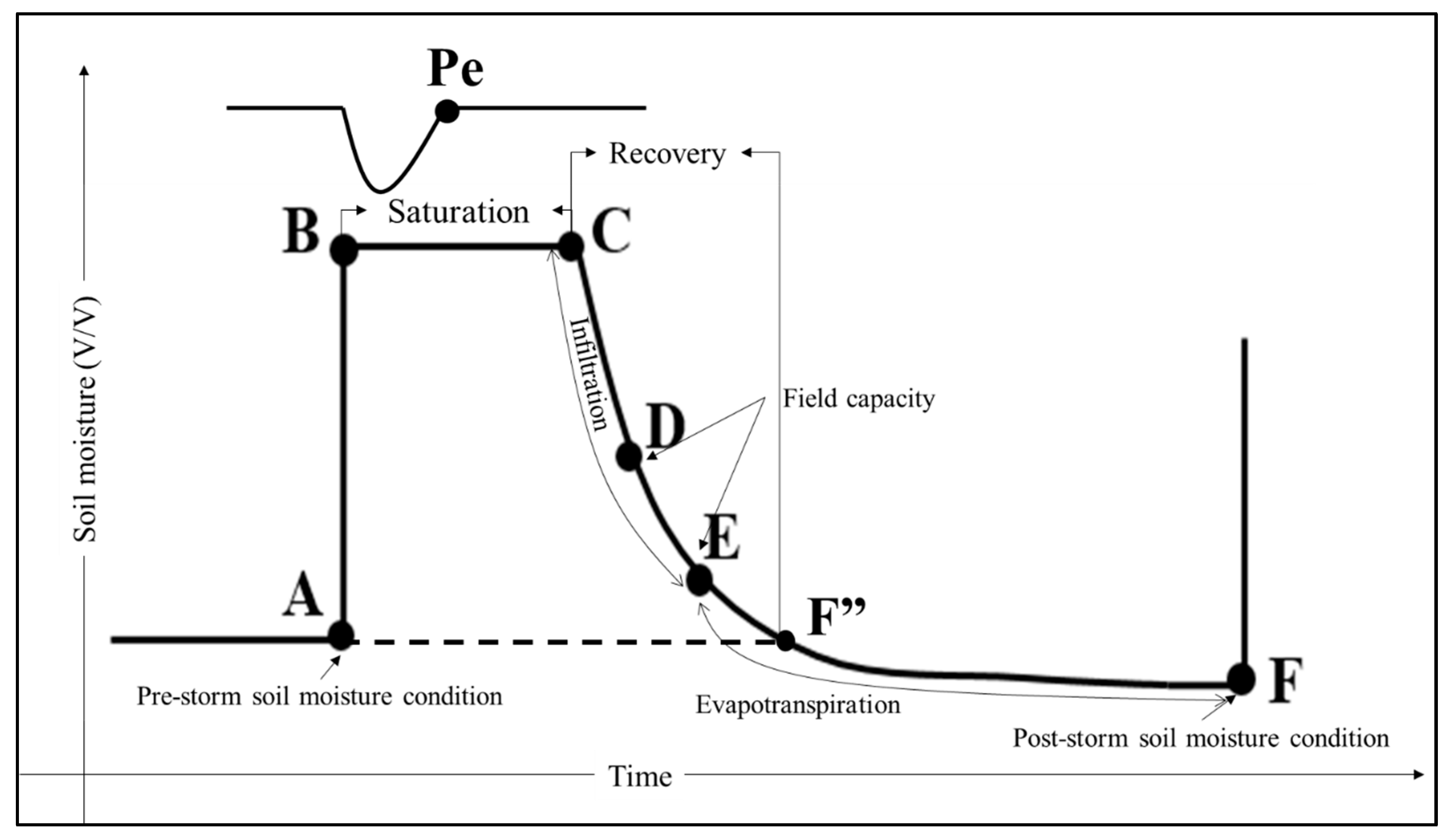
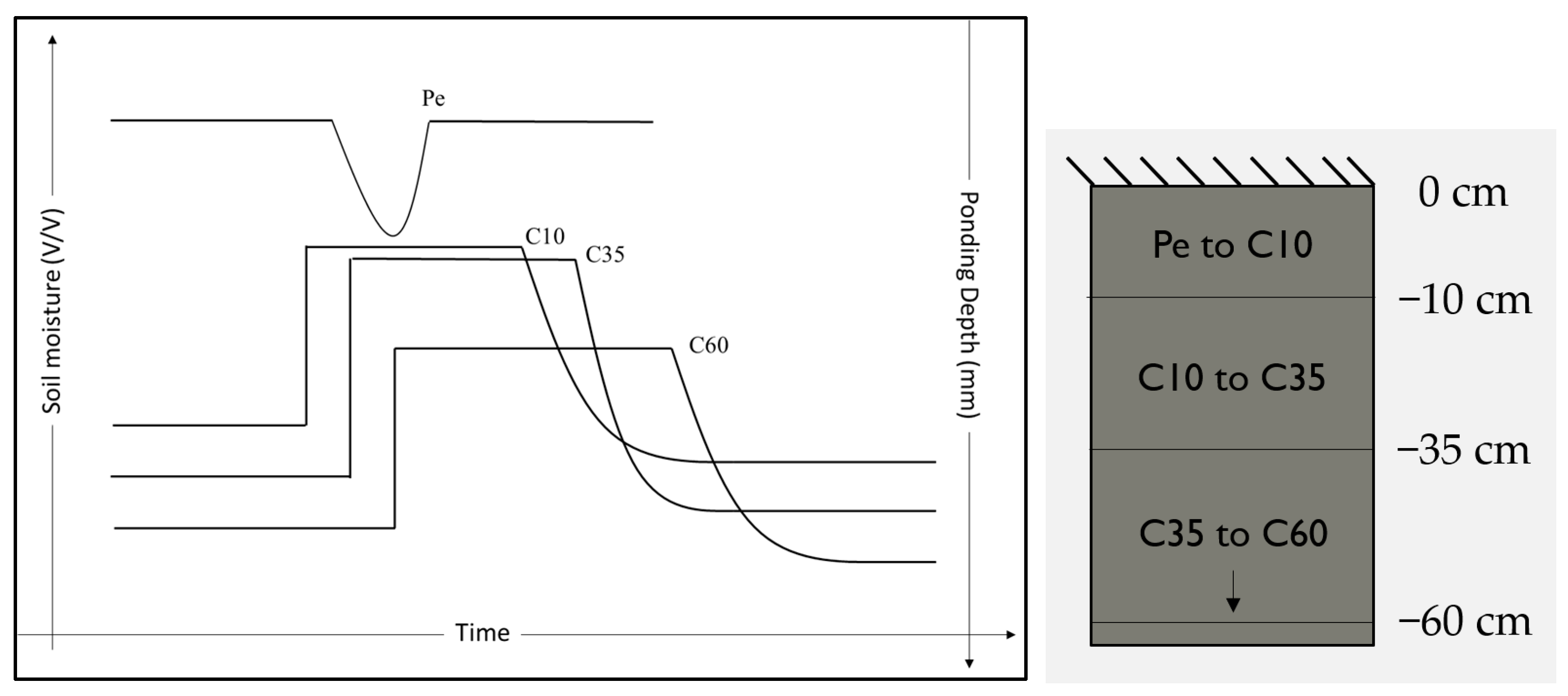
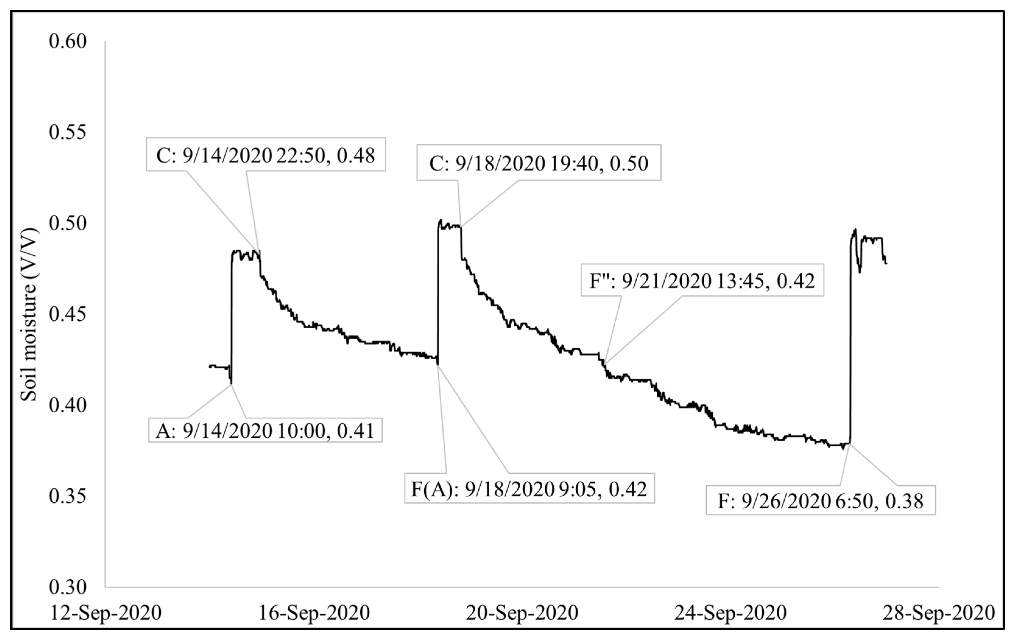
3.2. Soil Moisture Framework Definition

As the soil moisture data were analyzed, it was apparent from the consistent shape that was observed that there were changes in the rate that the soil moisture changed, which are the inflection points. For events that are selected, the inflection points in soil moisture are identified in the following way. The soil moisture increases from its pre-storm condition (defined as soil moisture inflection point A in conceptual framework, e.g., 0.304 volume/volume (v/v) in Figure 4) in response to a storm event. Then, the soil moisture quickly rises to reach a relative maximum (defined as soil moisture inflection point B, e.g., 0.466 v/v in Figure 4). During most observed events, once B is reached, the soil moisture continues to gradually increase until it reaches an overall maximum (defined as soil moisture inflection point C, e.g., 0.475 v/v in Figure 4) for that storm event. The small, gradual increase in soil moisture, if observed, from B to C is likely due to the release of entrapped air as saturation is extended over time. On the surface of the GSI, it is expected that ponding plays a role during this portion of the soil moisture conceptual framework, and, as such, the point in time where ponding ends (Pe) is cataloged.

After saturation is reached and the storm event ends (point C), the soil moisture recesses, quickly at first and then more gradually over time. From the observation of soil moisture recession curves, there are two inflection points that define a change in the slope in this curve (Figure 4). The first, relatively fast recession decreases to the inflection point D (e.g., 0.401 v/v in Figure 4) and then decreases more slowly to the inflection point E (e.g., 0.365 v/v in Figure 4), and finally decreases at a relatively slow and constant rate until the start of the next storm event (point F, e.g., 0.289 v/v in Figure 4). The change in the slope in soil moisture to identify point D ranged from 0.007 v/v to 0.035 v/v, while for point E this ranged from 0.003 v/v to 0.007 v/v. These points were not defined by a specific change in slope, but rather the change in slope was considered alongside the visual observation. The conceptual framework also includes another soil moisture point, F″, which is the equivalent soil moisture of point A (e.g., 0.304 v/v in Figure 4).

To conceptualize this behavior, a general visual of the soil moisture response before, during, and after a storm event is shown in Figure 5 with the A, B, C, D, E, F, F″, and Pe points defined. The time difference between point B and C is defined as the duration of saturation (e.g., 6 h for example presented in Figure 4). The duration of saturation can be used as an indicator of GSI performance as it is related to GSI ponding, which is a GSI design constraint as well as providing a duration of time that the soil is infiltrating at the saturated hydraulic conductivity.

For the recession limb of the soil moisture response, between points C and D, which are relatively quick, the dominating process is presumed to be infiltration where the soil moisture moves from saturated conditions towards field capacity conditions [4,5]. Points D and E represent a range of soil moisture values where field capacity conditions are likely met. To verify these field capacities soil moisture points, the soil water characteristic curve for the bioswale determined the water content at its corresponding water tension, which typically lies within the range of −6 kPa (61 cm suction) to −33 kPa (337 cm suction) depending on the texture, structure, and organic content of the soil [21,22]. Once the soil reaches field capacity, typically within a few hours for GSI soil, the recession rate slows and ET becomes the dominant factor in soil recovery [4,5]. The time associated with point F″ from point C is the recovery time. After point F″, if there is no rain and drying conditions, the soil moisture will continue to decrease until the next event, such that point F becomes point A of the next event.

3.3. Desaturation, Infiltration, and Evapotranspiration Analysis Using the Framework

A core concept of the soil moisture profile framework is to quantify the elapsed time that soil moisture is at each of the critical points (A, B, C, D, E, F, F″) determine important GSI processes such as infiltration, evapotranspiration, and time of desaturation.

For specific-system behavior with soil moisture sensors at multiple depths [9], the water movement through the soil column (or desaturation) can be tracked using the framework. Time of desaturation is defined to start at Pe and then tracked vertically down the soil column from the top to bottom sensor when point C is met. For example, the time between Pe and Point C for a soil moisture sensor at 10 cm depth (C10) is identified as the desaturation time for the top 10 cm of soil depth. Desaturation time can also be identified for soil layers between other soil moisture sensors such as 35 and 60 cm depth. For this framework, the duration of time from Pe to C10, C10 to C35, and C35 to C60 was obtained for the bioswale (Figure 6). A similar process was conducted for bioinfiltration but with 65 cm depth instead of 60 cm depth in the bioswale.

The rate of infiltration was calculated at each soil depth along the soil column based on the desaturation time of the soil layer (Equation (1)).

$$\mathrm{Infiltration} \mathrm{rate} \left(\frac{\mathrm{cm}}{\mathrm{h}}\right)=\frac{Soil Layer depth \left(\mathrm{cm}\right)}{Desaturation time \left(\mathrm{h}\right)}$$

(1)

For example, when water desaturates from Pe through to the top 10 cm, the infiltration rate is estimated as a ratio of the given soil depth (i.e., 10 cm) to the time taken by water to move from the surface to the desired depth (Equation (2)).

$$\mathrm{Infiltration} \mathrm{rate} \mathrm{at} 10 \mathrm{cm} \left(\frac{\mathrm{cm}}{\mathrm{h}}\right)=\frac{10 \mathrm{cm}}{\Delta T_{C10-Pe} \left(\mathrm{h}\right)}$$

(2)

where $\Delta T_{C10-Pe}$ represents the time difference between the end of ponding (Pe) and the time of soil moisture at Point C at 10 cm depth (C10). As the water moves along the soil column, i.e., 35 cm and 60 cm, the time difference is then the time taken by water to move from 10 cm to 35 cm $(\Delta T_{C35-C10} \mathrm{h})$ and 35 cm to 60 cm $(\Delta T_{C60-C35} \mathrm{h})$, respectively.

The ET rate is estimated using the difference in soil moisture from point E to F per the time taken by moisture to reach from point E to F along the root zone area. The root zone for each system was considered to reach the deepest soil moisture depth. For the bioswale, a 60 cm depth was used to estimate the ET rate (same as the depth of the engineered soil). Since there are three soil moisture sensors throughout the upstream and downstream column of the bioswale, each soil moisture depth was assumed to approximate about one third of the soil column (20 cm). The ET rate for the bioswale is estimated using Equation (3).

$$Bioswale ET rate \left(\frac{\mathrm{cm}}{\mathrm{d}}\right)=\frac{\Delta S{M}_{10}\left(E-F\right)}{\Delta T_{10} \left(E-F\right)}\times 20 \mathrm{cm}+\frac{\Delta S{M}_{35 }\left(E-F\right) }{\Delta T_{35} \left(E-F\right)}\times 20 \mathrm{cm}+\frac{\Delta S{M}_{60}\left(E-F\right)}{\Delta T_{60 }\left(E-F\right)}\times 20 \mathrm{cm}$$

(3)

where $\Delta S{M}_{10}\left(E-F\right)$ represents a change in soil moisture at 10 cm depth from point E to point F in v/v, and $\Delta T_{10} \left(E-F\right)$ represents the time difference from point E to point F at 10 cm depth in days. A similar definition is true for the other terms in Equation (3) for the different soil moisture depth of 35 and 60 cm. For ET estimation in the bioinfiltration, the root zone was assumed to be 65 cm as data are not available for deeper depths (although engineered media extends to 120 m), and one third of this depth (i.e., 21.7 cm) was applied to the soil moisture changes at 10, 35, and 65 cm.

3.4. Framework Validation

The soil moisture conceptual framework is validated through secondary data sources for the following parameters:

• Field capacity estimates (point D and E) verification through a soil water characteristic curve (SWCC) for both systems;
• System recovery determined through soil moisture recession comparison with a simulated runoff test (SRT) conducted at the bioswale;
• Infiltration estimates verified infiltration rate with spot field infiltration testing conducted at the bioswale;
• ET rate estimates compared to ET rates determined through a variety of other methods (such as lysimeter data) for both sites.

The SWCC curve, which defines the relationship between soil tension and soil moisture for unsaturated flow, was developed from data measured on a sample taken close to the 10 cm depth soil moisture sensor at the downstream part of the bioswale (collected in summer 2020) and bioinfiltration site (collected in fall 2015). The low suction, high water content side of the curve was estimated via data using the HYPROP device, and the high suction, low water content side of the curve was estimated via a WP4C device [23]. The data were fitted using an automated program that applies the van Genuchten curve fit [24].

The SRT was conducted on 14 September 2020 and 18 September 2020 in the bioswale. During this, the GSI was filled to full capacity with water.

Field spot infiltration tests were performed by SATURO infiltrometers to saturated hydraulic conductivity for both sites [16,19]. The geometric mean of the multiple spot tests (eight each for upstream and downstream in bioswale; six for biofiltration) is determined and compared with the framework estimates. For the bioswale site, spot field infiltration rates were determined over multiple seasons (see [16] for more information).

4. Results and Discussion

The framework was applied to two GSI systems for multiple soil moisture sensors within each GSI to determine the average soil moisture at each framework point, duration of saturation, soil moisture recovery, and estimation of infiltration and ET rates.

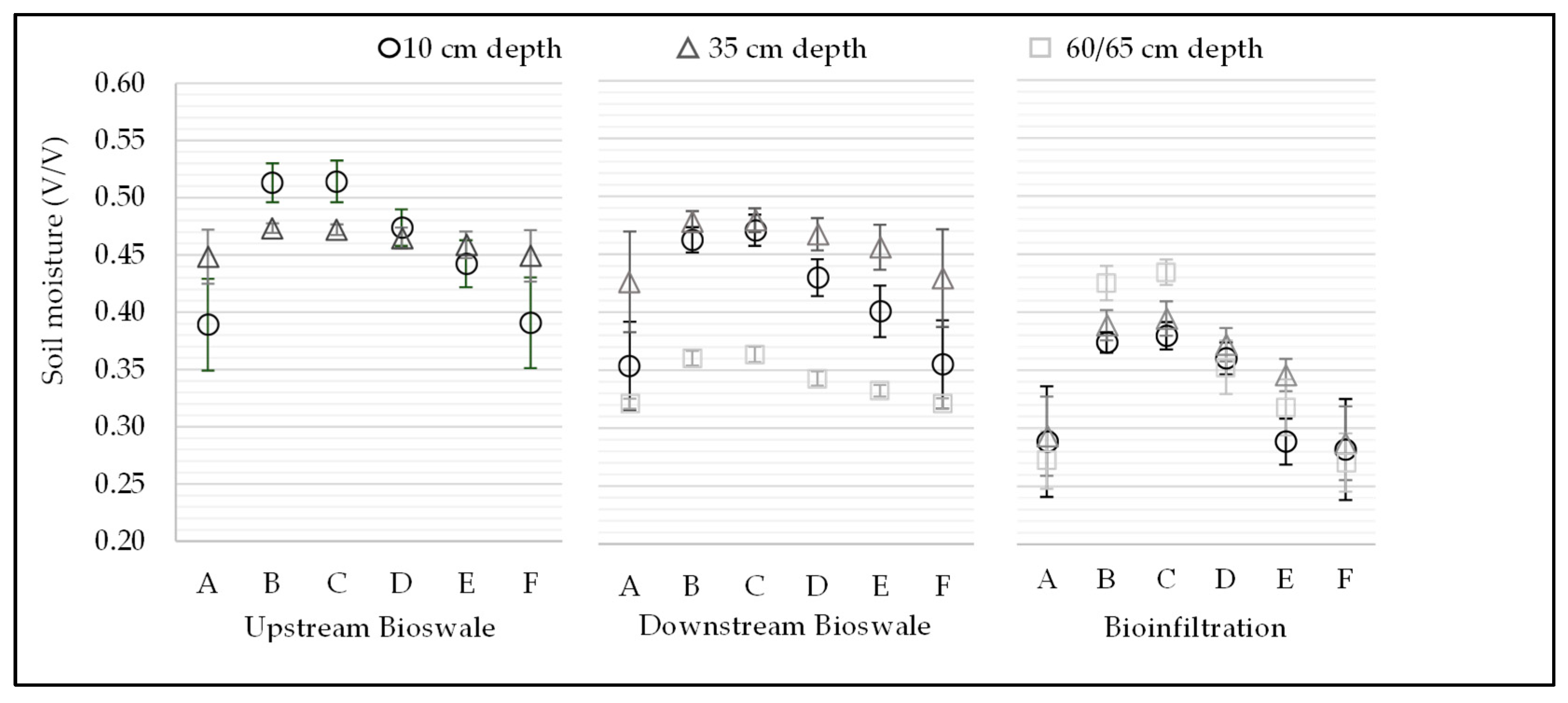
4.1. Soil Moisture Values for Conceptual Framework Points

For the bioswale, the soil moisture content at the six identified inflection points for the soil moisture framework (A, B, C, D, E, F) was obtained for 58 storm events at the upstream location from December 2019 to October 2020 and 54 storm events at the downstream location from September 2019 to October 2020. For the bioinfiltration site, the soil moisture content at the six identified points was obtained for 27 storm events from 2014 to 2018. For these selected storm events, the variation in soil moisture at different depths is shown in Figure 7. The soil moisture measurements indicate that there is the most variation in soil moisture at a 10 cm depth for all systems, especially points A and F. The 35 cm depths in all systems tend to show less variation compared to the 10 cm, and there is very little variation in the mean soil moisture at 60/65 cm depths for all framework points. This observation could be due to the proximity to the surface and sensitivity to ET and other atmospheric changes compared to the deeper sensors.

For the bioswale, the average moisture content at saturation (points B and C) is about 0.48 v/v based on 10 and 35 cm depths (in both upstream and downstream). The minor difference of about 0.05 v/v between saturation estimates (points B and C) between the 10 and 35 cm depth in the upstream bioswale is likely due to sensor variability. The mean saturated moisture content for a 60 cm depth downstream is 0.36 v/v, which is substantially lower than the other observations in the bioswale. The reason for this difference is likely due to the interaction of the interface of native media at the 60 cm depth, such as that the native soil has lower saturated hydraulic conductivity compared to the placed media, or that the roots are not reaching this depth, or a combination of both factors, which causes the deepest depth in the soil column to stay wetter for longer periods compared to the upper depths.

For the bioinfiltration site, the average saturated moisture content for all depths ranged between 0.38 and 0.43 v/v, with a similar difference of 0.05 v/v seen in the bioswale and likely due to sensor variability. The behavior of the 65 cm depth is much more similar to the trend in points A, B, C, D, E, and F for the other depths in the bioinfiltration. This is a notable difference from the behavior of the deepest sensor at 60 cm depth in the bioswale, where there are much more subtle changes. This is likely due to the deeper depth of the bioinfiltration media (120 cm) and perhaps a reflection of a less restrictive native media in terms of infiltration rate compared to the bioswale.

On average, moisture contents range between 0.51 and 0.32 v/v for all points in the bioswale, whereas they range from 0.43 to 0.27 v/v in the bioinfiltration, which is likely due to the sandier soil type (loamy sand in the bioswale versus the sandy loam in the bioinfiltration). While soil moisture sensor readings are not necessarily exact, the soil moisture framework was able to be applied to two different systems and provide estimates on saturation, showing differences between soil types and useful context for underlying drainage. This application indicates that the framework is generic enough to be transferable to other vegetated GSI systems and may enable the identification of soil conditions.

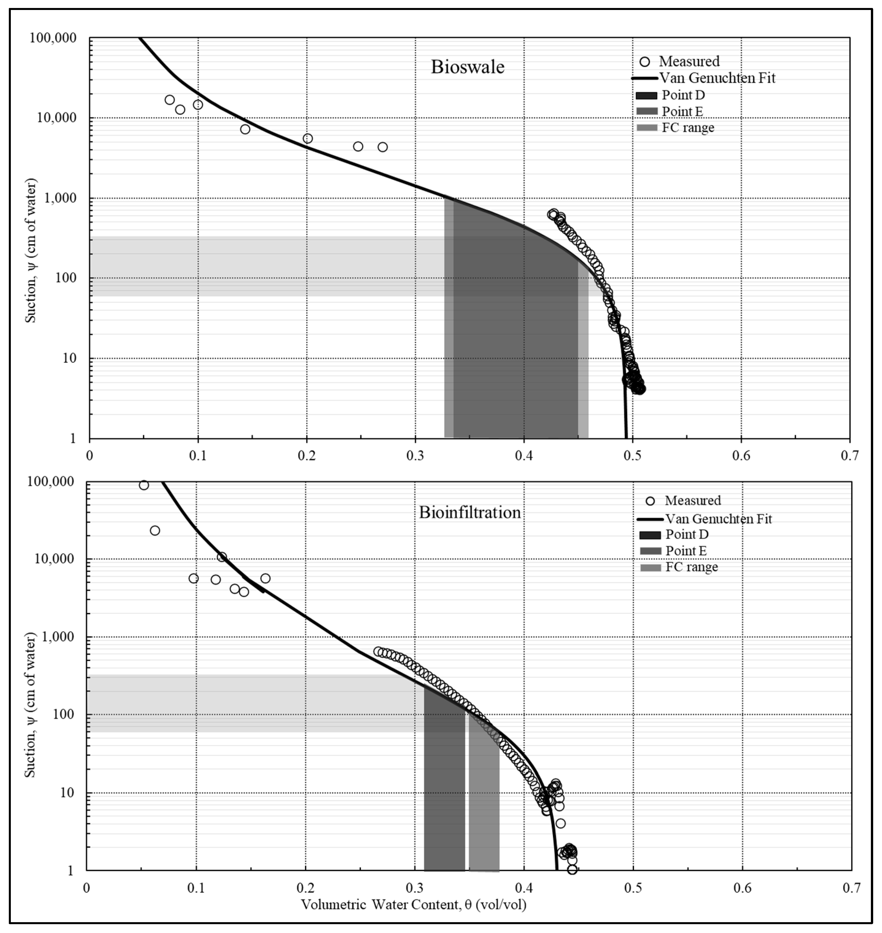
4.2. SWCC Field Capacity Comparison to Framework Points D and C

Point D and E of the framework were selected as the inflection points along the recession side of the soil moisture response to represent the field capacity (FC). The traditional FC is often thought as a singular soil moisture point correlated to the suction of 337 cm suction on an SWCC; however, others define FC as within the range of 61–337 cm suction [21,22] as FC depends on the texture, structure, and organic content of the soil. This FC range is used to compare the range of point D and E of the framework as loose compaction and organic content are the key aspects of GSI soil (Figure 8).

The conceptual framework point D and E for the downstream bioswale range from 0.34 to 0.47 v/v and 0.33 to 0.46 v/v, respectively, for all depths, which corresponds to the suction range between 100 and 1000 cm (Figure 8, upper). This range partially falls along the FC tension range of 61–337 cm suction; however, it is important to consider the effects of including the 60 cm depth’s points D and E as they are much lower than the upper depths, as discussed in the previous section. If 60 cm depth were excluded from this comparison, the range of points D and E reduce to 0.40 to 0.46 v/v, which corresponds to a suction between 100 and 400 cm suction, where a much more similar range to what [21,22] recommends (i.e., 61–337 cm suction) would be found.

The conceptual framework point D and E for the bioinfiltration range from 0.35 to 0.37 v/v and 0.29 to 0.35 v/v, respectively, for all depths, which corresponds to the suction range between 60 and 200 cm (Figure 8, lower). This range fully overlaps with the range [21,22] recommended (i.e., 61–337 cm suction). In general, the range of point D (shaded light grey in Figure 8) and point E (shaded dark grey in Figure 9) overlap with the FC range of 61 to 337 cm suction (shaded mid-grey in Figure 8) for both GSI sites. As such, this indicates that point D and E in the framework aid in the determination of field capacity.

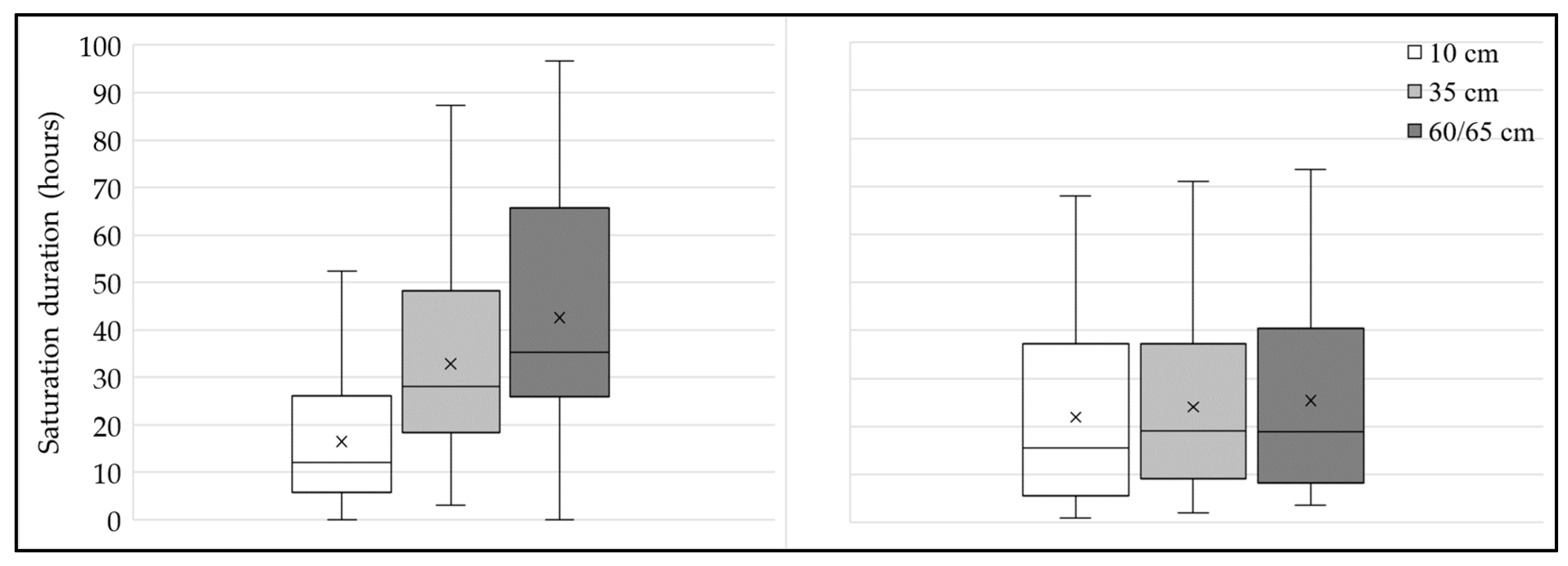
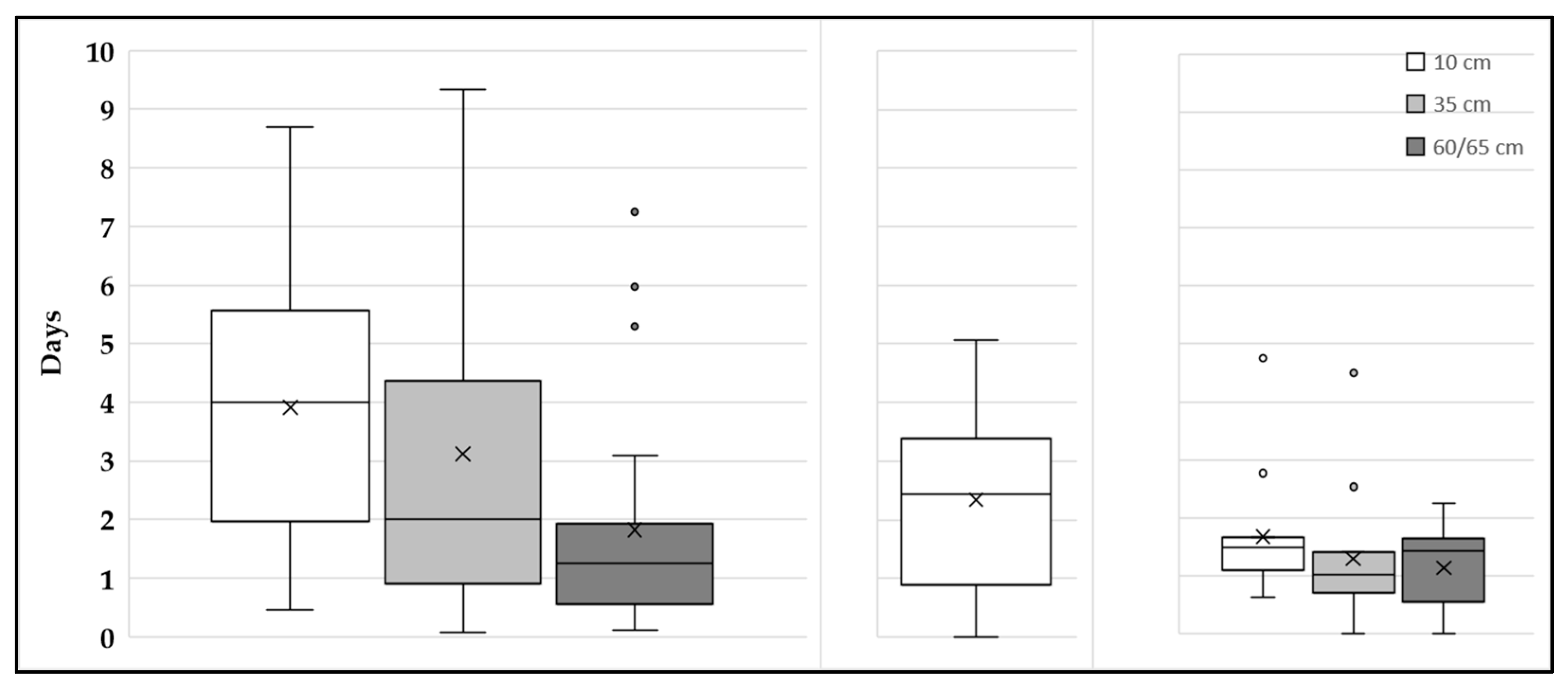
4.3. Duration of Saturation

Utilizing the framework, the downstream bioswale remained saturated for an average of 16 h, 30 h, and 37 h for 10 cm, 35 cm, and 60 cm, respectively (Figure 9, left). For the bioinfiltration site, the system remained saturated on average for 16 h, 19 h, and 19 h, respectively for 10 cm, 35 cm, and 65 cm (Figure 9, right). For the bioswale, the average duration of saturation increased with depth in a statistically significant way, whereas the duration of saturation for the bioinfiltration stayed the same with depths with no statistical difference.

This difference between the two systems is likely due to the drainage differences between the systems (as described in Site Description, the bioswale has a gentle surface slope), but may also have a do with the media depths of the systems (i.e., 60 cm for bioswale and 120 cm for biofiltration). The bioinfiltration site is twice as deep as the bioswale media, although the comparison depths are relatively the same. If an increase in the duration of saturation with depth is occurring in the bioinfiltration site, it may not be captured at 65 cm depth or the bottom boundary of the bioinfiltration may not be as limiting as the bioswale site.

The average time (±standard deviation) it took for water to move from the surface (Pe) of the downstream part of the bioswale to 10 cm down was 4.2 h (±5.4 h). Similarly, it took an average of 14.6 h (±11 h), and 9.6 h (±6.4 h) for water to move from 10 to 35 cm depth and 35 to 60 cm depth, respectively. It was found that surface ponding ended at the same time that end of saturation (point C) was reached at 10 cm for the bioinfiltration. Due to this, water movement was analyzed between 10 cm and 35 cm and between 35 and 65 cm. The average time taken by the water to move from 10 to 35 cm and 35 to 65 cm for the bioinfiltration is 2.6 h (±2.7 h) and 1.8 h (±1.4 h), respectively. Despite the bioswale having a sandier soil (loamy sand vs. sandy loam) and a higher saturation (0.48 v/v vs. 0.40 v/v on average for top two depths), indicating a larger void space compared to bioinfiltration, the movement of water through the downstream bioswale system is slower than the bioinfiltration. As the bioinfiltration site is an older GSI with more established vegetation (a tree) in comparison to the bioswale, the bioinfiltration system is likely benefitting more from preferential flow paths that enable the movement of water through the system quicker than the downstream bioswale.

4.4. Soil Moisture Recession Analysis

The average recession time based on the framework is estimated from point C (end of saturation) until point F″, which indicates the time it took for the GSI system to fully recover from its pre-storm condition. This was performed for all sites and sensor depths except for upstream 35 and 60 cm due to datalogging issues. The average recessions (±standard deviation) for the downstream bioswale estimated at 10 cm, 35 cm, and 60 cm depths are 3.9 ± 2.3 days, 3.1 ± 2.8 days, and 1.8 ± 2.0 days, respectively (Figure 10). The upstream bioswale averaged recession time based on the 10 cm sensor is 2.5 ± 1.5 days (Figure 10). For the bioinfiltration site, the average recession times estimated for 10 cm, 35 cm, and 65 cm are 1.7 ± 1.1 days, 1.4 ± 1.1 days, and 1.4 ± 0.5 days, respectively (Figure 10). Recession time is variable due to seasonal effects, the definition of recession/recovery in the framework as it is dependent on pre-storm conditions, and the storm event itself (e.g., volume). It is notable that the recession time in the bioinfiltration site is consistent (approx. 1.5 days) with depth, whereas the recession time in the downstream bioswale decreases with depth. This is likely due to the increase in saturation conditions with soil depth in the downstream bioswale system, which affects the pre-storm condition and definition of recovery to the wet pre-storm condition.

To understand if the recession based on the 10 cm depth of the downstream bioswale (i.e., 4 days) is indicative of recovery, the results from two SRT performed 4 days apart (14 September 2020 and 18 September 2020) at the bioswale are compared (Figure 11). The SRT is the process where inflow is artificially introduced to the bioswale until the soil is completely saturated and outflow is observed at the outlet, which allows for the influence of storm-based variabilities to be excluded. Initial moisture conditions for both SRTs were similar (0.41 v/v and 0.42 v/v for 14 September and 18 September, respectively—Figure 11). Although by the definition of the framework, this is not fully recovered in between the time, it was close enough to validate that the time of 3.5 days (between point C and F in the framework) was approximately enough for the site to recover between tests similar to the four-day average indicated by the framework. After the second SRT, it took less than three days for the system to recover (i.e., recess to its pre-storm condition) based on the 10 cm depth. After the SRTs, a storm event of 18 mm depth occurred on 26 September 2020, 8 days after the second SRT. Point F for this storm is defined at 0.28 v/v, demonstrating the dependency of the pre-storm condition in the framework. Overall, the back-to-back SRTs also demonstrate that downstream bioswale performed well qualitatively.

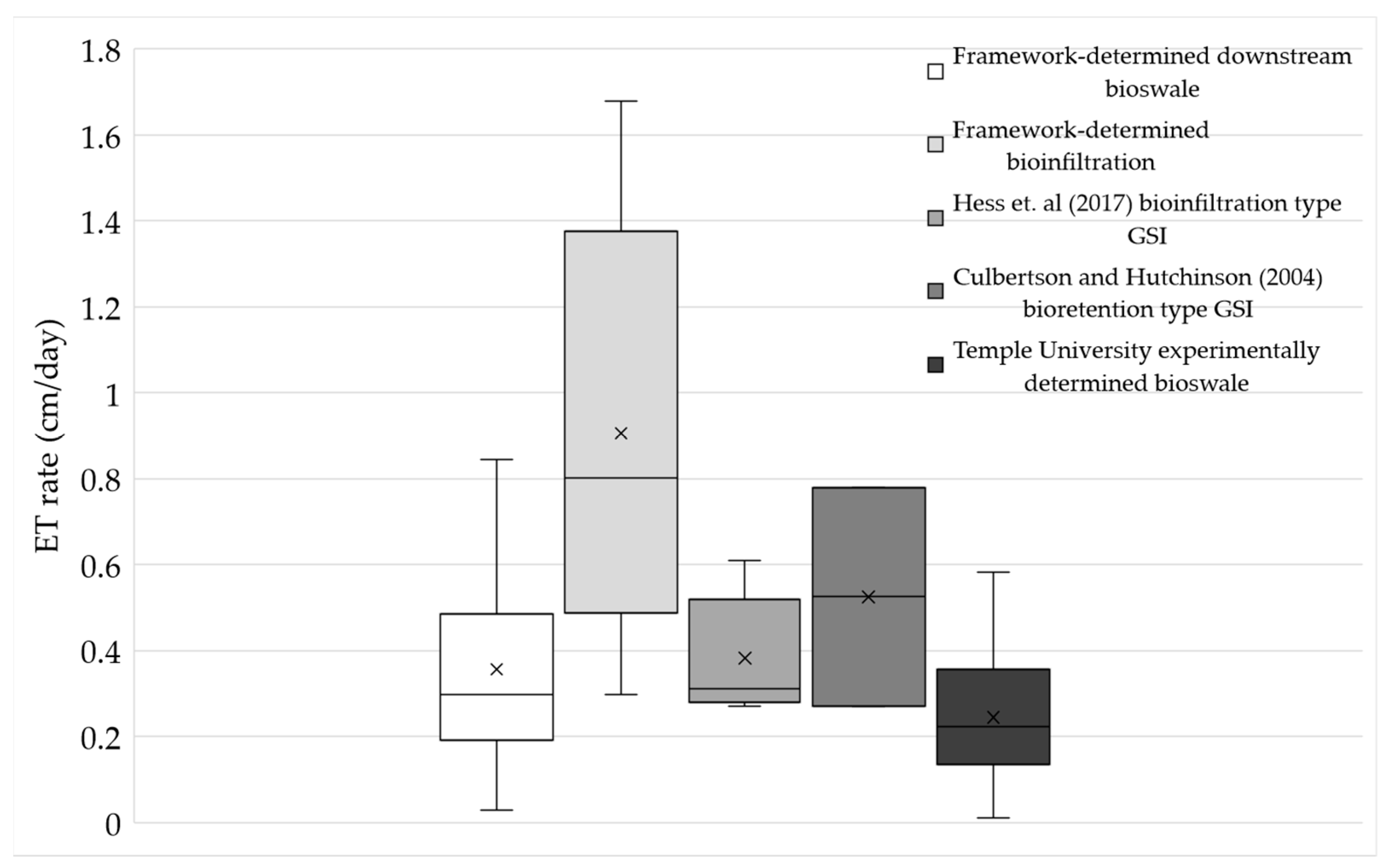
4.5. Framework Determined Infiltration and ET and Comparison

Point E in the framework is identified as the point used to distinguish ET-dominated and infiltration-dominated behavior in the GSI system. Infiltration rates were estimated using Equation (1) (Equation (2) being a specific example for 10 cm depth in the bioswale), and ET rates were estimated using Equation (3) for the bioswale. A similar process was performed for bioinfiltration. The average infiltration rate based on the movement of water between the surface (Pe) and 10 cm depth, 10 cm and 35 cm, and 35 cm and 60 cm sensors for bioswale is 5 cm/h, 3 cm/h, and 4 cm/h, respectively (

Table 1. Seasonal analysis of framework-determined infiltration and ET rates at downstream bioswale.

Season	Average Framework Infiltration Rate Estimates (cm/h)			Average Framework ET Rate Estimates (cm/day)
	(Change in Pe to C10)	(Change in C10 to C35)	(Change in C35 to C60)	(Change in Point E to F of 10 cm Depth Sensor)
Fall 2019	4.7 (n = 5)	3.7 (n = 10)	8.0 (n = 10)	0.27 (n = 11)
Winter 2019	0.8 (n = 3)	1.4 (n = 8)	1.9 (n = 8)	0.17 (n = 7)
Spring 2020	2.6 (n = 2)	1.5 (n = 13)	3.2 (n = 11)	0.37 (n = 13)
Summer 2020	7.9 (n = 7)	4.5 (n = 12)	5.7 (n = 12)	0.79 (n = 10)
Fall 2020	4.3 (n = 7)	2.2 (n = 7)	3.4 (n = 7)	0.86 (n = 7)
All Seasons	4.9 (n = 24)	2.7 (n = 50)	4.4 (n = 46)	0.48 (n = 48)

). Based on analysis performed at this site by [16], these rates align well with the average spot field estimates of saturated hydraulic conductivity of about 5–7 cm/h in summer and 3.5–4 cm/h in fall. Further, infiltration and ET rates varied with season at the downstream bioswale. The highest framework determined infiltration and ET rates was observed in summer and lowest in winter, as expected (Table 1). The average infiltration rate based on the movement of water between the 10 cm and 35 cm and 35 cm and 60 cm sensors for bioinfiltration is 16 cm/h and 19 cm/h, respectively (

Table 2. Average framework-determined infiltration and ET rate at bioinfiltration.

Average Framework Infiltration Rate Estimates (cm/h)		Average Framework ET Rate Estimates (cm/day)
(Change in C10 to C35)	(Change in C35 to C65)	(Change in Point E to F of 10 cm Depth Sensor)
16 (n = 24)	18 (n = 19)	0.91 (n = 23)

). Based on the analysis performed at this site by [19], these framework-determined rates are within the range of the average spot field estimates of saturated hydraulic conductivity of 11 cm/h, 18 cm/h, and 30 cm/h during fall 2018, summer 2019, and fall 2019, respectively. Based on these results, the framework-determined infiltration rates are similar to the field measured saturated hydraulic conductivity for both sites and therefore provide a method for understanding the average saturated hydraulic conductivity, a key performance indicator, of GSI.

The framework-determined average ET rates for bioswale and bioinfiltration are 0.48 cm/day and 0.91 cm/day, with a range of 0.3–1.7 cm/day, respectively. The range of the framework-determined ET rates of both systems is compared to the GSI ET estimates from the literature and other research (Figure 12). The three sources from the literature include: a lysimeter representing a bioinfiltration GSI with 61 cm of sand media at a nearby site at Villanova, PA, which had an average ET rate of 0.39 cm/day and an ET rate range of 0.27–0.61 cm/day [3,25], a bioretention system in Canada studied by [26] which found a range of 0.27–0.78 cm/day, and finally Temple University conducted research on the bioswale in this study, which determined an average ET rate of 0.25 cm/day and a range of 0.01–0.58 cm/day (between 8 June and 22 September 2019). A study conducted by [8] found ET rates for two urban bioinfiltration sites in New York City to be with 0–0.97 cm/day and 0–0.93 cm/day, respectively.

The range and average ET rate estimated using the conceptual framework for downstream bioswale and bioinfiltration were both compared to Temple University’s experimentally determined ET using a statistical model (Caplan et al., in prep) that was developed through a static flux chamber measurement of H₂0 accumulation (ET) with a gas analyzer on the same site. The lysimeter-determined ET derived from a bioinfiltration-type GSI in the same state to provide a comparison for the bioinfiltration system. However, the bioinfiltration system had much higher rates of ET compared to the other systems. This is likely due to the established vegetation in the bioinfiltration, which started in 2003 and has experienced an evolution of dense vegetation and a tree in the middle of the pond over two decades [27].

5. Conclusions

Within stormwater engineering design, we do not have one standard approach to describing subsurface hydraulics. Frequently used models such as Green-Ampt are used, but they do not typically align with field observations nor aid in advancing GSI soil dynamic understanding. A novel conceptual framework of soil moisture behavior under pre-, during-, and post-storm conditions is presented that begins to respond to this gap. A framework of seven points (A, B, C, D, E, F, F″) was established to separate regions of soil water behavior in the subsurface layer in green stormwater infrastructures. They represented pre-storm (point A), post-storm (point F), saturation (point B and C), field capacity (point D and E), and soil moisture recession (F″). Based on the framework, the soil moisture points were studied for one year of data for a bioswale in Philadelphia, PA, and selected events for a bioinfiltration SCM in Villanova, PA. These defined soil moisture points were used to monitor the subsurface hydrology of the same GSI units that included average soil moisture measurements, duration of saturation, soil moisture recession, desaturation time, infiltration rates, and ET rates.

The application of framework in estimating a field capacity range (point D and E) for both systems aligned well with a field capacity range of 61–337 cm suction [21,22] based on an SWCC developed for both soil medias. Using the framework, average ET rates of 0.48 and 0.91 cm/day were determined for two different GSI systems, a bioswale and bioinfiltration, respectively. The bioswale ET rates were comparable to other ET measurement methods for similar systems. The bioinfiltration ET was higher than the bioswale, which is likely due to the establishment of a tree within the system. The framework-determined infiltration rates for both sites (4.9 cm/h for bioswale and 16 cm/h for bioinfiltration) were comparable to the field spot saturated hydraulic conductivity tests (5.1 cm/h for bioswale and 11–30 cm/h for bioinfiltration).

This framework provides a structure to understand soil moisture measurement output that is agnostic to the actual soil moisture values, which are known to be a temperamental field measurement. Thus, regardless of sensor value, the application of the soil moisture conceptual framework provides an understanding of the system’s longevity to hold water and its recovery process, the relationship between soil and water, thus providing information on the dynamics of water within the soil layer, and site-specific soil conditions, including changes in performance over time. The soil moisture profile, which is the varying water availability over time, needs to be better quantitatively understood as it allows us to obtain detailed knowledge of the soil–water dynamics, which are a function of design choices, system maintenance success, and local site conditions. While this framework includes the full storm cycle, emphasis is placed on the points of saturation, system recovery, infiltration, and evapotranspiration of the soil moisture profile as these are the primary indicators of GSI performance, system health, and demonstrates system recovery. As maintenance continues to be a substantial factor in the success of stormwater management programs that rely on GSI [28], having another tool of using soil moisture to indicate when maintenance is required is extremely helpful.

The present work demonstrates the usefulness of the framework to understand a GSI systems’ response and recovery (including consistency of responses) to storm events. This framework was developed based off a bioswale site but was able to be transferred to another GSI site, a biofiltration system, with a different soil type, depth, and drainage, and still enabled understanding of subsurface hydrology. Moving forward, others could use this framework and their own site data to develop a site-specific curve. Another possible use of this framework is to use the values found here to help guide modeling or design efforts that use a continuous simulation approach. Overall, this framework is effective at understanding the efficacy of GSI and quantifying the difficulty of determining key aspects of unit processes (such as ET and infiltration) that enable GSI to function long-term.

References

1. Amur, A.; Wadzuk, B.; Traver, R. A 15-Year Analysis of Precipitation and Rain Garden Response. Hydrol. Process. 2022, 36, e14736. [Google Scholar] [CrossRef]
2. Berland, A.; Shiflett, S.A.; Shuster, W.D.; Garmestani, A.S.; Goddard, H.C.; Herrmann, D.L.; Hopton, M.E. The Role of Trees in Urban Stormwater Management. Landsc. Urban Plan. 2017, 162, 167–177. [Google Scholar] [CrossRef] [PubMed]
3. Hess, A.; Wadzuk, B.; Welker, A. Evapotranspiration in Rain Gardens Using Weighing Lysimeters. J. Irrig. Drain. Eng. 2017, 143, 04017004. [Google Scholar] [CrossRef]
4. Hess, A.; Wadzuk, B.; Welker, A. Evapotranspiration Estimation in Rain Gardens Using Soil Moisture Sensors. Vadose Zone J. 2021, 20, e20100. [Google Scholar] [CrossRef]
5. DelVecchio, T.; Welker, A.; Wadzuk, B.M. Exploration of Volume Reduction via Infiltration and Evapotranspiration for Different Soil Types in Rain Garden Lysimeters. J. Sustain. Water Built Environ. 2020, 6, 04019008. [Google Scholar] [CrossRef]
6. Traver, R.G.; Ebrahimian, A. Dynamic Design of Green Stormwater Infrastructure. Front. Environ. Sci. Eng. 2017, 11, 15. [Google Scholar] [CrossRef]
7. Nichols, W. Modeling Performance of an Operational Urban Rain Garden Using HYDRUS-1D. Master’s Thesis, Villanova University, Villanova, PA, USA, 2018. [Google Scholar]
8. DiGiovanni, K.A. Evapotranspiration from Urban Green Spaces in a Northeast United States City. Ph.D. Thesis, Drexel University, Philadelphia, PA, USA, 2013. [Google Scholar]
9. Shakya, M.; Traver, R.G.; Wadzuk, B. Monitoring Infiltration Movement through the Soil Profile in Urban Rain Gardens. In Proceedings of the Low Impact Development Conference, Nashville, TN, USA, 12–15 August 2018; Volume c, pp. 9–15. [Google Scholar]
10. Le Morvan, A.; Zribi, M.; Baghdadi, N.; Chanzy, A. Soil Moisture Profile Effect on Radar Signal Measurement. Sensors 2008, 8, 256–270. [Google Scholar] [CrossRef] [PubMed]
11. Romero, D.; Torres-Irineo, E.; Kern, S.; Orellana, R.; Hernandez-Cerda, M.E. Determination of the Soil Moisture Recession Constant from Satellite Data: A Case Study of the Yucatan Peninsula. Int. J. Remote Sens. 2017, 38, 5793–5813. [Google Scholar] [CrossRef]
12. Campbell Scientific. CS 700—L Rain Gage with 8 in Orifice; Campbell Scientific: Logan, UT, USA, 2020. [Google Scholar]
13. American Sigma. Rain Logger Automatic Data Logging Rain Gauges; American Sigma: Ronkonkoma, NY, USA, 2001. [Google Scholar]
14. Campbell Scientific. CS451/CS456 Submersible Pressure Transducer; Campbell Scientific: Logan, UT, USA, 2022. [Google Scholar]
15. Stevens Hydraprobe. Soil Probe—Stevens Hydra Probe II; Stevens Hydraprobe: Portland, OR, USA, 2018. [Google Scholar]
16. Smith, C.; Connolly, R.; Ampomah, R.; Hess, A.; Sample-Lord, K.; Smith, V. Temporal Soil Dynamics in Bioinfiltration Systems. J. Irrig. Drain. Eng. 2021, 147, 1–15. [Google Scholar] [CrossRef]
17. Calt, E.D. Comparing the Hydrologic Performance of a Linear Cascading Bioswale to Traditional Bioinfiltration in a Highly Urbanized Setting: An Integrative Approach Investigating Modeling, Design, and Construction. Master’s Thesis, Villanova University, Villanova, PA, USA, 2018. [Google Scholar]
18. Jenkins, J.K.G.; Wadzuk, B.M.; Welker, A.L. Fines Accumulation and Distribution in a Storm-Water Rain Garden Nine Years Postconstruction. J. Irrig. Drain. Eng. 2010, 136, 862–869. [Google Scholar] [CrossRef]
19. Mckane, I.H. Temporal Trends in Infiltration, Soil Texture, and Nutrient Accumulation in Rain Gardens. Master’s Thesis, Villanova University, Villanova, PA, USA, 2020. [Google Scholar]
20. Emerson, C.; Traver, R.G. The Villanova Bio-Infiltration Traffic Island: Project Overview. In Proceedings of the Critical Transitions in Water and Environmental Resources Management, Salt Lake City, UT, USA, 27 June 2004; pp. 1–5. [Google Scholar]
21. De Oliveira, A.; Ramos, M.M.; de Aquino, L.A. Irrigation Management. In Sugarcane Agricultural Production, Bioenergy and Ethanol; Academic Press: Cambridge, MA, USA, 2015; pp. 161–183. [Google Scholar]
22. Peng, Z.; Smith, C.; Stovin, V. The Importance of Unsaturated Hydraulic Conductivity Measurements for Green Roof Detention Modelling. J. Hydrol. 2020, 590, 125273. [Google Scholar] [CrossRef]
23. Meter Group. User Manual HYPROP; Meter Group: Pullman, WA, USA, 2017; ISBN 5702012100. [Google Scholar]
24. Seki, K.; Toride, N.; van Genuchten, M.T. Closed-Form Hydraulic Conductivity Equations for Multimodal Unsaturated Soil Hydraulic Properties. Vadose Zone J. 2022, 21, e20168. [Google Scholar] [CrossRef]
25. Wadzuk, B.M.; Hickman, J.M.; Traver, R.G. Understanding the Role of Evapotranspiration in Bioretention: Mesocosm Study. J. Sustain. Water Built Environ. 2015, 1, 1–7. [Google Scholar] [CrossRef]
26. Culbertson, T.L.; Hutchinson, S.L. Assessing Bioretention Cell Function in a Midwest Continental Climate. Am. Soc. Agric. Biol. Eng. 2004, 7841–7852. [Google Scholar]
27. Jahangiri, H.M. An Automated Method for Delineating Drainage Areas of Green Stormwater Infrastructures Using GIS. Master’s Thesis, Villanova University, Villanova, PA, USA, 2018. [Google Scholar]
28. Wadzuk, B.; Gile, B.; Smith, V.; Ebrahimian, A.; Strauss, M.; Traver, R. Moving Toward Dynamic and Data-Driven GSI Maintenance. J. Sustain. Water Built Environ. 2021, 7, 02521003. [Google Scholar] [CrossRef]
Figure 1. Conceptual representation of soil moisture response to a storm event.
Hydrology 10 00197 g001
Figure 2. Images of vegetation in bioswale upstream (left) and downstream (middle) as well as the bioinfiltration site (right).
Hydrology 10 00197 g002
Figure 3. Example of storm event selection process for conceptual framework.
Hydrology 10 00197 g003
Figure 4. Example of soil moisture response at 10 cm depth for downstream bioswale resulting from storm on 28 August 2020.
Hydrology 10 00197 g004
Figure 5. Definition of A, B, C, D, E, F, F″ point in conceptual framework of soil moisture in response to a storm event.
Hydrology 10 00197 g005
Figure 6. Conceptual representation of soil moisture sensors response to a rainfall at multiple depths within the soil column (left) and sketch of soil column.
Hydrology 10 00197 g006
Figure 7. Mean soil moisture measurement at points A, B, C, D, E, and F for the upstream and downstream portion of the bioswale and bioinfiltration sites. Whiskers indicate minimum and maximum soil moisture values of soil moisture measurements.
Hydrology 10 00197 g007
Figure 8. Framework point D and point E range compared to SWCC field capacity (FC) range for bioswale (upper) and bioinfiltration (lower).
Hydrology 10 00197 g008
Figure 9. Box plots of duration of saturation for downstream bioswale (left) and bioinfiltration (right) at each soil depth. The middle line is mean, × indicates median, upper, and lower box which are interquartile range, and the line that extends the box is whiskers, which represent datasets outside the interquartile range (covers datasets that are ±1.5 times the interquartile range). The data outside the whiskers are outliers.
Hydrology 10 00197 g009
Figure 10. Box plots of recession for downstream bioswale (left) upstream bioswale (middle) and bioinfiltration (right) at soil depths. The middle line is mean, × indicates median, upper, and lower box which are the interquartile range, and the line that extends the box is the whiskers, which represent datasets outside the interquartile range (covers datasets that are ±1.5 times the interquartile range).
Hydrology 10 00197 g010
Figure 11. Soil moisture response to SRTs that were performed 4 days apart followed by a storm event on 26 September 2020 with framework points A, C, F, and F″ denoted.
Hydrology 10 00197 g011
Figure 12. Framework-determined ET rate for downstream bioswale and bioinfiltration compared with other GSI ET estimates and research.
Hydrology 10 00197 g012