1. Introduction
Climate change is a significant threat to humanity and the Earth’s ecosystems in the 21st century. The challenge of climate change has been long-term. However, the world needs urgent action to maintain a sustainable future for the Earth [
1]. One of the most significant climate changes in the world’s oceans is SLR. The main reasons for SLR are the thermal expansion of the oceans, ice loss from glaciers, melting ice sheets, and changes in land-water storage. SLR affects the low-lying coastal areas, defined as the zones below 10 m elevation above sea level. It is known that a significant proportion of the global population (almost 11%) is living on low-lying coasts [
2]. SLR impacts the coastal ecosystems and the economic activities of these areas negatively (loss of habitat and species; loss of fish stocks; loss of agricultural areas due to frequent flooding; loss of fresh water; loss of cultural and natural heritage), thus decreasing their resilience to climate change. Low-lying lands are among the habitats on Earth most vulnerable to climate change effects. Even if the heating of the Earth stops, these areas will still be facing those threats beyond 2100 [
3].
It has been reported that the global mean sea level increased by 0.20 m between 1901 and 2018. SLR is accelerating as the average rate of SLR was 1.3 mm/yr between 1901 and 1971, 1.9 mm/yr between 1971 and 2006, and 3.7 mm/yr between 2006 and 2018. The projections of SLR in the 21st century are carried out for different scenarios. These scenarios are based on Shared Socioeconomic Pathways. It is expected that under the very low Greenhouse Gas (GHG) emissions scenario (SSP1-1.9—where the global net CO
2 emissions are cut to net zero by 2050), SLR by 2100 is expected to be 0.28–0.55 m, whereas it is expected to be 0.63–1.01 m under the very high GHG emissions scenario (SSP5-8.5—where the global net CO
2 emissions double by 2050). However, it is also possible to see a global mean SLR of 2 m by 2100 under a very high GHG emissions scenario due to the uncertainty in ice-sheet melting processes [
4]. SLR is predicted to continue for thousands of years. It has been modeled that SLR will be about 2 to 3 m if warming is limited to 1.5 °C, 2 to 6 m if limited to 2 °C, and 19 to 22 m with 5 °C of warming for the next 200 years [
5].
As for the regional seas, a few studies exist about the climate change effects on the Black Sea. Ceyhunlu et al. [
6] investigated the climate change effects on the sea surface temperatures and wind speeds of the Western Black Sea Coast of Turkey. They applied and compared Sen’s Innovative Method and Trend Analysis Methods (Mann–Kendall and Spearman’s Rho Methods). Their study showed that for all provinces of the Western Black Sea Coast, there is an increasing trend of high levels of Sea Surface Temperature (15–27 °C). Dabanlı et al. [
7] focused on sea surface temperature (SST) trends along the Black, Marmara, Aegean, and Mediterranean coastal areas in Turkey. SST data are categorized into five clusters considering fish life as “hot”, “warm-hot”, “warm”, “cold”, and “very cold”. For the Black Sea region, they have concluded that for the summer, “warm-hot” and “hot” temperatures increase rapidly by +3% in the form of a positive trend. For the winter season, they showed that SST measurements have descending trends. They have concluded that extreme events in the winter season are more frequent than the past cases on the Black Sea coasts. Görmüş and Ayat [
8] studied the coastal vulnerability of the Southwestern Black Sea. They included geomorphology, coastal slope, shoreline change, wave height, mean beach width, SLR, population density, and land use as the physical and social variables affecting the vulnerability. They produced a vulnerability map of the study area using a Coastal Vulnerability Index (CVI).
As for the Black Sea, there are several specific studies regarding the SLR projections. Ginzburg et al. [
9] studied the inter-annual changes in the sea level anomalies of the Black Sea and the Azov Sea for the years 1993–2020. They showed that the average SLR for the 1993–2020 period is +0.32 ± 0.16 cm/year, which is 1.5 times more than from the 1920s to the mid-1990s (0.17–0.18 cm/year). Lebedev et al. [
10] studied the Northeastern part of the Black Sea and showed that for the time interval of 1993–2015, SLR has a rate of 0.29 ± 0.03 cm/yr. Avşar and Kutoğlu [
11] have concluded that the mean SLR rate for the Black Sea is 2.5 ± 0.5 mm/yr by using the gridded satellite altimetry data for 1993–2017. Dayan et al. [
12] studied high-end SLR scenarios (HESs) for global and (some) regional coastal areas. They based their projections on model projections for glaciers, ocean sterodynamic effects, glacial isostatic adjustment, and land–water contributions. They also relied on a “recent expert elicitation assessment” for Greenland and Antarctic ice sheets. Two emission scenarios and three time horizons are considered (2050, 2100, and 2200). They have concluded that, for HESs-A, the global mean sea level (GMSL) is projected to reach 1.06 (1.91) in the low (high) emission scenario by 2100. For HESs-B, GMSL may be higher than 1.69 (3.22) m by 2100. They have also studied several regional coastal areas. For these areas, they have shown that, for HESs-A, the mean sea level (MSL) is projected to reach 0.48 (1.20) in the low (high) emission scenario by 2100. For HESs-B, MSL may be higher than 1.14 (2.46) m by 2100. Görmüş and Ayat [
8] projected that the relative SLR for the Black Sea would be within ±20% of the global mean. Therefore, in this study, three scenarios of SLR (1 m SLR, 2 m SLR, and 3 m SLR) by 2100 are considered for the Karasu coastal area.
This study aims to determine the risk maps and vulnerability–hazard maps of the Karasu coastal area due to different SLR scenarios. SLR scenarios for the Karasu coastal area were built on 1 m, 2 m and 3 m by 2100. The presented work here can be viewed as a first integrated assessment for the policymakers and stakeholders of the Karasu coastal area concerning the risks and hazards of probable SLR scenarios. The risk maps present features at risk (exposure indicators). The effect of SLR on the GDP and population density of the Karasu coastal area is also studied. The combined hazard–vulnerability map presents the land loss caused by inundation due to SLRs. The vulnerability indicates the specification of the risk area caused by the hazard element, which causes casualties of the people, their properties, and land use as well [
13]. In order to reach this goal, probable land loss due to SLR scenarios were analyzed by GIS approaches [
14]. The analysis is used to determine the coastal vulnerability aspects, creating maps representing the coastal risks [
15]. All the data required were collected related to the research objectives. DEM as input information is extracted from 11 topographic sheet maps output at a nominal scale of 1:5000, issued by the General Directorate of Land Registry and Cadaster in Turkey [
16]. The land use data in this research was obtained from the Landsat 8 satellite imagery collected on 13 April 2017 (path/row-179/031). The satellite imagery was recorded in Geo-TIFF format with a resolution of 30 m (cell size X, Y = 30 m) and was retrieved from the Earth Explorer website [
17]. As conventional data, the OpenStreetMap data set was collected to excerpt the study area roads [
18]. SLR projected data was utilized from the existing studies [
19,
20,
21].
2. The Study Area
Karasu Town, located along the Black Sea, is the most responsive land spreading along the southern Black Sea shore and is the biggest settlement of the Sakarya Province (
Figure 1) [
22]. The Karasu coastline lies mainly from the Sakarya River mouth to the Maden Stream mouth. The Sakarya River is the largest river in western Anatolia and is named the third longest river in Turkey, following the Kızılırmak and the Fırat Rivers. The Sakarya River is a crucial source of domestic and irrigation water, demonstrating its enormous capacity to generate energy, and it delivers alluvial components for arable land. The climate of the study area falls within the Marmara Transition type of the humid Black Sea climate with an annual average temperature of 13 °C and a total amount of rainfall of 805.1 mm. Annual prevailing wind direction has been detected as Northeast (NE) direction. The study area contains a topographic diversity, including a beach, a lake, coastal terraces, fills, and hilly terrains [
23].
Regarding vegetation, it is located within the Euxine province of the European Siberian phytogeographic area. The increasing agricultural activities have destroyed humid forests, which grew depending on the climatic conditions. The urbanization density reaches around 35% around the shore of Karasu. There is a significant migration increase to the city center from the rural areas. Karasu is a maritime transport and merchant center as well as a popular tourism destination with the most important resorts on the Western Black Sea, making tourism the primary economic income of the city [
24]. In 1996, a fishing pier was started around the area of 1 km to the east. Later, the construction was modified to a harbor and finished in 2008 [
25]. In order to prevent coastal erosion due to the construction of the harbor, twelve 25 m long groins were constructed in 2009. In addition, a total of nine 120 m offshore breakwaters with a distance of 75 m were constructed between 2010 and 2012 as an additional solution for coastal erosion. The coastal erosion in the Karasu coastal area has been studied in several studies [
22,
23,
24,
25,
26,
27,
28].
3. Materials and Methods
In order to achieve the targets mentioned above, several approaches have been carried out. The first was to create a DEM to accomplish the coastal inundation maps, which involve using an SLR data set to identify and estimate the inundation levels in the future. The second significant approach was to use satellite images in order to delineate land use to create an exposure indicator surface on behalf of each of the features at risk (exposure indicators), such as urban areas, roads, forests, natural vegetation and agricultural lands, water bodies, sandy beaches, GDP, and population. These form the site’s detailed information to overlay the inundation maps for calculating and evaluating the potential effects of projected inundation. The overall approaches followed in this study are presented in detail below.
3.1. Formation of Borders and Shorelines
The coastline of the study area was extracted from Local Vector Shoreline LVS using the Landsat 8 satellite imagery. Additionally, the study area was identified by a shape file of boundary, which is used as a mask to obtain and calculate the total area for the chosen exposure indicators. This operation was applied to mask 3, 4, and 5 bands of Landsat 8 satellite image data that was extracted before exporting it to ENVI 5.3 to classify the satellite image. Thus, exposure indicators are obtained.
3.2. Creating DEM
In coastal studies, the most widely-spread dataset is the DEM. Elevation models are necessary for assessing the risk of inundation from tsunami, storm surge, and sea-level increase. Occasionally, DEMs are used as input in complex simulation models that forecast flooding and other coastal hydrological processes. Additionally, DEM is a base layer in a simple GIS “bathtub” flooding analysis [
29,
30]. The elevation in each cell is compared to a predicted sea level, and all cells with values lower than the foreseen sea level are considered flooded [
19].
Some DEMs are derived from LiDAR (Light Detection and Ranging), a remote sensing technology that measures the distance to ground targets. For instance, Poulter and Halpin [
31] have utilized LiDAR elevation data to perform sea-level rise simulations on the North Carolina coast. Another commonly accepted source of data elevation is the U.S. Geological Survey’s National Elevation Dataset (NED), which is used in SLAMM (Sea-Level Affecting Marshes Model), a simulation model which studies wetlands’ response to long-term sea-level rise [
32]. Nonetheless, these datasets feature limited vertical accuracies: the NED is accurate to ±2.4 m [
33] and LiDAR elevation data is accurate from 15 cm to 1 m [
34]. Scientists estimate a sea-level rise of up to 1 m by 2100 [
35]. Performed by these datasets, simulations of sea-level rise results must be precisely analyzed. In the future, GIS and remote sensing applications in coastal studies will benefit significantly from widely assessable elevation data with increased vertical accuracy and the development of more refined coastal vulnerability indicators. The accuracy of coastal elevation data needs to be within centimeters for sea-level rise inundation models to predict flooding and other impacts effectively.
In this study, DEMs result from 11 topographic sheet maps covering approximately 12 × 7 km
2 with a nominal scale of 1:5000. These maps are issued by the General Directorate of Land Registry and Cadaster in Turkey [
16]. The maps consist of contour lines and points collected through contour maps by manual digitizing methods. ArcMap10.0 software was employed to process and interpolate DEM data, involving the geocoding in UTM cartographic projection Zone 36N-Datum D_WGS_1984 switched to the ArcMap data format and combined to comply with the study area border in the ArcGIS environment.
In order to obtain our DEM, the methodology presented by Blomgren [
36] was followed. It is well known that DEM is an image indicating the elevation values at each x and y position. In the implementation of DEM, it is stated that there are three phases: data acquisition, interpolation, and manual editing of the resulting elevation map if needed. The DEM parameters are 3.77 m × 3.77 m in the x-y plane and 0.45 m in the z-direction. Therefore, the model can capture the narrow features in the horizontal plane. The resulting DEM is presented as a contour plot in
Figure 2 and forms a proper base for visualizing inundation scenarios.
3.3. Feature Extraction with an Object-Based Classification Approach
A study dedicated to coastal processes involves the analysis of both conventional and casually sensed data. Conventional data is more precise and site-specific. On the other hand, data collection is time- and cost-consuming; it involves more labor and might not apply to more extensive areas. However, remotely sensed data is quick and economical due to repeated and synoptic coverage of the vast and hard-to-access areas [
38]. Remote Sensing and GIS tools can be applied to form land use, land cover, and coastline change detection maps [
39]. In the presented study, both conventional and remotely sensed data were used. The land use data applied in this research was obtained from the (Landsat 8 OLI) satellite imagery. The land use of the area and coastal waterways are depicted based on Feature Extraction such as natural vegetation and agricultural lands, forest, roads, urban spreading, sandy beaches, and water bodies. An object-based approach to classify imagery is demonstrated. An object (also called a segment) is a group of pixels with analogous spectral, spatial, and texture attributes utilizing image unsupervised classification on the ENVI 5.3 software. As conventional data, OpenStreetMap data [
18] are obtained to excerpt the study area roads. Overall, map accuracy of 83.33% has been obtained based on 42 ground truth points by using the Create Random Points tool in ArcMap and then interpreting from high-resolution aerial image. Finally, the classified image has been converted into vector format for further analysis.
3.4. Modelling of Inundation Zone
SLR accelerates erosion and flooding in coastal areas. Coastal areas characterized by cliffs, bluffs, and coastal mountains are more vulnerable to coastal erosion due to elevated sea levels. Coastal plains are under more risk of permanent flooding due to wave action, storm surge, and hurricanes under SLR [
40].
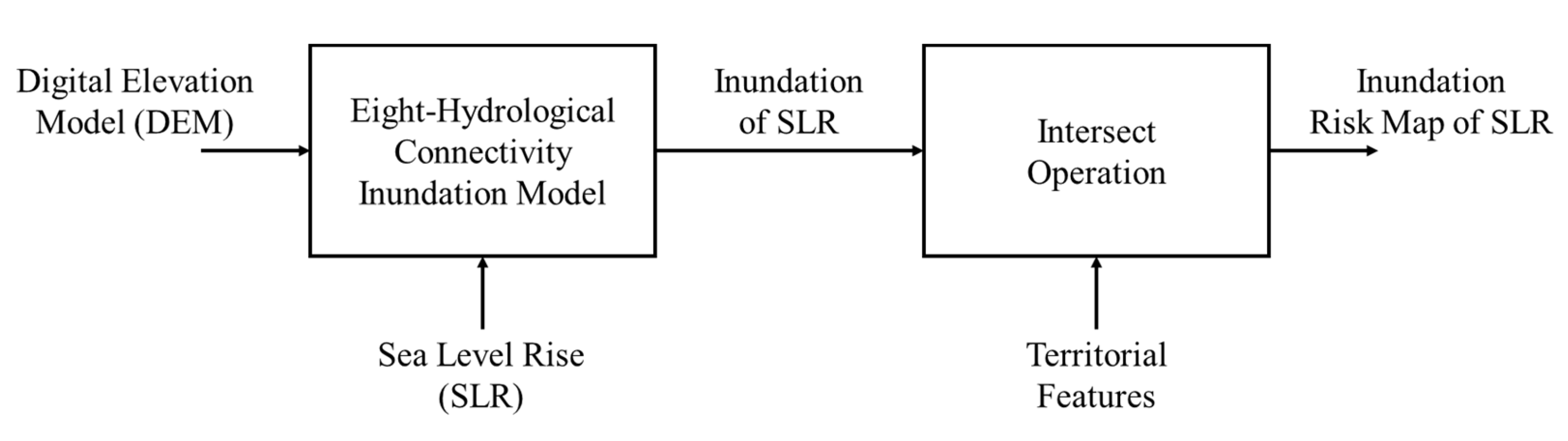
The model utilized in this research given by Snoussi et al. [
41,
42] calculates inundation zones and their risk maps which provide information for decision-makers. The main phases of Model Builder are shown in
Figure 3. In
Figure 3, SLR values are chosen as 1 m, 2 m, and 3 m for three different inundation scenarios and the territorial features correspond to the forest, water bodies, vegetation, population, GDP, sandy beach, roads, and urban areas. The model processing is supported by ArcMap 10.0 software by uniting coastal spatial data with SLR projections of 1 m, 2 m, and 3 m, respectively [
19,
20]. This analysis contributes to identifying and ranking areas that will probably be influenced by sea-level rise. The approach used to model hydrological connectivity is referred to as the eight-side rule, suggested by Poulter and Halpin [
31]. The inundation simulation is applied by using DEM. The equation below describes the usage of the model to expect inundation:
F takes only two values: flooded, represented by 1, or not flooded by 0. is the elevation at locations x and y, is SLR projection, and C represents connectivity which is 1 (connected) or 0 (not connected).
Once a condition is met, F is indicated with a ‘true’ and takes 1; otherwise, F is indicated with a ‘false’ and takes 0. This indicates the potential (1) and unlikely (0) pixel locations. Hence, bitmaps of the criteria are used to select possible areas that are to be inundated. Furthermore, when the elevation is under sea level, the grid cell will be flooded if it is linked to another flooded grid cell nearby, wherever the grid cell was joined if its cardinal and diagonal trends were joined to a flooded grid cell. This output map represents the hazard map of the Karasu coastal area due to SLR at 1, 2, and 3 m. The accuracy of connectivity of the surface is influenced by the connectivity rule selected and the resolution of DEM. Then, once again, ‘Bitmaps’ as input maps are combined with each exposure indicator (Land use map) using “Boolean AND” operation (Boolean Overlay), which is an intersection of binary-coded data layers (inundation zones & exposure indicators). This creates a binary output map representing potential pixel locations containing value 1. The resulting output map shows the places satisfying all criteria needed for this application. It also represents the risk maps of inundation levels for SLR at 1, 2, and 3 m.
3.5. Combination of the Hazard Map with Vulnerability Map
Vulnerability measures the potential adverse effects of a hazard on human and coastal systems. Vulnerability indicates the specification of the risk area caused by hazard elements, which causes casualties of the people and their properties and land use [
20]. In a related context, Aydın and Uysal [
15] calculated the vulnerability of the Karasu region’s coastline. According to the characteristics of its coast, it was classified into 21 points and then subdivided into seven sections.
Aydın and Uysal [
24] found that the vulnerability of the coastline was, in turn, scored from 1 to 3 (with 1, 2, and 3 representing low, medium, and high vulnerability, respectively) for each section, allowing the vulnerability, V, to be calculated by Equation (2). The results are given in
Table 1.
where P
d is the population density, P
g is the per capita GDP, and C
f is the coastal function [
15].
Their output summarized that the coastline of the study area is sensitive, with low and medium vulnerability according to the vulnerability score mentioned earlier. In this study, the vulnerability values of the seven sections given in
Table 1 were assigned to represent the vulnerability map of the Karasu coastline. Consequently, this output result (vulnerability map) was combined with the coastal hazard map obtained from the discussion in
Section 3.4. In the second step, the vulnerability map is combined with the hazard map using the Overlay operation.
4. Results
In order to determine the beachfront elevation of the Karasu coastal area, the aforementioned digitized DEM model is utilized.
Figure 4 illustrates the low-lying land zones of the Karasu coastal area, which are broader on the western shore.
Figure 4 also demonstrates the possible zones which are vulnerable to flooding due to SLR. Additionally, GIS modeling is used to determine the anticipated inundation levels of 1 m, 2 m, and 3 m by 2100. SLR scenarios are applied along the coast of Karasu City, where the horizontal flood depth at some points extends more than 100 m inland, reaching some residential areas and the city’s road network. The vulnerability of a coastal area to SLR depends not only on physical characteristics such as elevation, geomorphology, shoreline change, wave height, tidal range, and rate of SLR but also the society’s capacity to respond to the dynamic changes in these features in terms of preventive and mitigation measures [
43].
The significant outcomes of land loss caused by inundation levels of 1, 2, and 3 m are presented in
Figure 5. The green, yellow, and red areas show the flooded areas for 1 m, 2 m, and 3 m SLR, respectively. As seen from
Figure 5, the most notable changes happen in the Sakarya River mouth and around the western and eastern parts with low-lying land and natural coastal defenses such as dunes.
Table 2 gives a detailed picture of the inundated areas to emphasize the differences between the inundation levels of SLRs. Roads are excluded from the area calculations, and the inundation values for roads are given in length. As is seen from
Table 2, the significant effect of SLR on the exposure indicators starts with 2 m level.
Table 3 gives the effect of SLR scenarios based on population and GDP. The population of the Karasu Coastal Area is 59,130 people, and the GDP per capita is 14,600 USD [
44].
The Karasu coastal zone elevation to SLR was demonstrated by means of DEM data and GIS models using the Equation (1). This demonstration represents the projected inundation level of 1 m, 2 m, and 3 m. Overlaying (intersecting) the inundated zones (hazard map) with the relevant exposure surface dataset (receptors) was calculated using eight parameters: Urban areas consisting of downtown as a core and its outskirts, roads, forest, natural vegetation and agricultural lands, aquatic bodies, sandy beaches, GDP, and population. These parameters are considered in the image classification using ENVI software and result in the intersect operation producing risk maps for each indicator.
The risk maps presented in
Figure 6 show the affected regions for three SLR scenarios of six different receptors (vegetation, urban areas, sandy beach, water bodies, forests, and roads). The green, yellow, and red areas show the flooded areas for 1 m, 2 m, and 3 m SLR, respectively.
Figure 7 represents the combination of the hazard map with the vulnerability data of Aydın and Uysal [
15]. The combined hazard and vulnerability map shows that 78% of the Karasu coastline has a medium vulnerability. The coastal areas behind the medium vulnerable coastlines show more inundation levels for coastal areas behind low vulnerable coastlines.
5. Discussion
As can be seen from
Figure 6a, in the 3 m SLR scenario, most of the vegetation areas are inundated for the 2 m SLR scenario, the vegetation area at the Sakarya River mouth is at risk, and for the 1 m scenario, the risk is low.
Figure 6b shows the risk map of urban areas. Urban areas undergo risk for 1 m and 2 m SLR. The risk for urban areas is especially significant, starting from 2 m SLR.
Figure 6c shows the risk map of the sandy beach. As expected, the beach is jeopardized at 1 m SLR.
Figure 6d shows the risk map of water areas. There are two river mouths in the region. One is the Sakarya River mouth and to the west of it is the Maden Stream mouth. Both of these water bodies are entirely at risk starting from 1 m SLR. This risk is not limited to water bodies but results in the salination of freshwater resources and loss of arable land and has a negative effect on the existing ecosystems.
Figure 6e shows the risk map of forests. Since forests are located in the mountains, which lie parallel to the coastline, these are areas at low risk.
Figure 6f shows the risk map of roads at 1 m SLR: the roads at the coastline are at risk. 2 m SLR covers most of the roads along the coastal area. From
Figure 7, it is seen that estuarine areas at the west and east of the Karasu region have a medium vulnerability. In contrast, the inland behind the coastal zone has a low vulnerability.
According to the results of this study, the total inundated areas are discussed as follows: The 1 m SLR scenario indicates that approximately 1.4% of the total land area would be impacted, including urban areas, natural vegetation, agricultural lands, beaches, and river mouth. In the 2 m SLR scenario, there is a vast increment of the zone that would be influenced by this rate compared to the inundation level of 1 m to reach 6%. It impacts urban and coastal territories and expands to low-lying zones, especially in the western part, covering 75 m from the river’s end, including natural vegetation and agricultural lands, beaches, and forests. In the 3 m SLR scenario, approximately 29% of coastal land will face a risk of inundation in the western and eastern parts, including the front exterior of Karasu City, harbors and the tourist resorts, natural vegetation and agricultural land, beaches and coastal dunes, woodlands, rivers, and water bodies. Such a loss of land suggests that the population living directly in these territories would retreat. The area least vulnerable to inundation is the beachfront strip which is restricted and is upheld by the slight height of the local location of the city of the residential area. Nonetheless, some parts of Karasu City, including its harbor and important recreational beaches, will be inundated.
It is also seen from
Table 2 that the significant effect of SLR on the exposure indicators starts with the 2 m level. The vegetation and urban areas show an inundation increase of almost 10 times for 2 m SLR. Roads show a five-times higher value for the same level. For the 3 m SLR scenario, almost half of the Karasu region is inundated, concerning exposure indicators. One interesting result is for the vegetation and forests, where almost 25% of these areas suffer from 3 m SLR. These areas are almost safe for the 1 m and 2 m scenarios. These results agree with the geographical characteristics of the Karasu coastal area. It can be seen from
Table 3 that 11,132 people will experience flooding in the extreme case, which will cause a GDP loss of 162,527,200 USD.
6. Conclusions
In this paper, an overall analysis of SLR has been carried out to assess the risk of low-lying coastal areas in the Karasu region in Turkey. SLR scenarios for Karasu coastal area are studied for 1 m, 2 m, and 3 m by 2100. As a result of this research, determinable data is developed on the effect of SLR on the Karasu coastal area. Inundation levels were visualized using DEM. The outcomes of GIS-based inundation maps indicated 1.40%, 6.02%, and 29.27% of the total land area for 1 m, 2 m, and 3 m SLR scenarios, respectively. The most notable changes are predicted to happen in the Sakarya River and Maden Stream mouths and around western and eastern parts of this area with low-lying land and natural coastal defenses such as dunes.
The minimum inundation level in a 1 m SLR scenario indicates that the most affected exposure indicators would be water bodies, sandy beaches, and roads. For the 2 m SLR scenario, there is a vast increment of the zone that would be influenced. It impacts not only urban and coastal territories but also expands to some low-lying zones, especially in the western part, covering a 75 m long area from the end of the river, including natural vegetation and agricultural lands, beaches, and roads. At the maximum inundation level in a 3 m SLR scenario, the coastal land will face a risk of inundation in the western and eastern parts, including the coastline of Karasu City, the harbor, the tourist resorts, natural vegetation and agricultural land, beaches and coastal dunes, woodlands, roads, rivers, water bodies, and forests. The middle section between the two river mouths and behind the coastal zone of the Karasu Region is found to have the minimum risk with regard to SLR inundation scenarios. From the combined hazard–vulnerability map, it is seen that estuarine areas at the west and east of the Karasu region have a medium vulnerability. In contrast, the inland behind the coastal zone has a low vulnerability. Such a loss of land suggests that the population living directly in these inundated territories would have to move out or retreat. The effect of SLR scenarios based on population and GDP shows that 11,132 people will experience flooding in the extreme case, which will cause a GDP loss of 162,527,200 USD.
This study has some limitations. The model assumes a fixed shoreline (the model excludes the shoreline change due to erosion/accretion). Additionally, the effect of storm surge is also excluded. Therefore, for future studies, it is suggested that an SLR model including shoreline evolution and storm surge can be developed. However, the presented model is a first for the Karasu coastal area. Karasu is the biggest settlement in the Sakarya Province. It is an imperative summer resort city where tourism is a major economic activity with resorts in the west of the Black Sea, as well as a maritime transport and trade centre, which also provides significant financial profit. The presented work here can be viewed as a first integrated assessment for the policymakers and stakeholders of the Karasu coastal area about the risks and hazards of probable SLR scenarios. These results can provide primary assessment data for the Karasu region to the decision-makers to enhance policies and planning of land use and to build a long-term policy for coastal management.
Author Contributions
Conceptualization, H.T. and A.N.G.; methodology, A.E., H.T. and A.N.G.; software, A.E. and H.H.M.; validation, A.E., A.N.G. and H.T.; formal analysis, A.E. and H.T.; investigation, A.E.; resources, H.T. and H.H.M.; data curation, A.E., A.N.G., H.T. and H.H.M.; writing—original draft preparation, A.E., A.N.G. and H.T.; writing—review and editing, A.E., A.N.G. and H.T.; visualization, A.E., A.N.G., H.T. and H.H.M.; supervision, A.N.G., H.T. and H.H.M.; project administration, H.T. and A.N.G.; funding acquisition, H.T. and A.N.G. All authors have read and agreed to the published version of the manuscript.
Funding
This research received no external funding.
Data Availability Statement
Data is unavailable due to privacy restrictions.
Conflicts of Interest
The authors declare no conflict of interest.
References
- Masson-Delmotte, V.; Zhai, A.P.; Pirani, S.L.; Connors, C.; Péan, S.; Berger, N.; Caud, Y.; Chen, L.; Goldfarb, M.I.; Gomis, M.; et al. (Eds.) IPCC, 2021: Summary for Policymakers. In Climate Change 2021: The Physical Science Basis; Contribution of Working Group I to the Sixth Assessment Report of the Intergovernmental Panel on Climate Change; Cambridge University Press: Cambridge, UK; New York, NY, USA, 2021; pp. 3–32. [Google Scholar] [CrossRef]
- Glavovic, B.C.; Dawson, R.; Chow, W.; Garschagen, M.; Haasnoot, M.; Singh, C.; Thomas, A. 2022: Cross-Chapter Paper 2: Cities and Settlements by the Sea. In Climate Change 2022: Impacts, Adaptation and Vulnerability; Contribution of Working Group II to the Sixth Assessment Report of the Intergovernmental Panel on Climate Change; Pörtner, H.-O., Roberts, D., Tignor, M., Poloczanska, E., Mintenbeck, K., Alegría, A., Craig, M., Langsdorf, S., Löschke, S., Möller, V., et al., Eds.; Cambridge University Press: Cambridge, UK; New York, NY, USA, 2022; pp. 2163–2194. [Google Scholar] [CrossRef]
- Oppenheimer, M.; Glavovic, B.; Hinkel, J.; van de Wal, R.; Magnan, A.; Abd-Elgawad, A.; Cai, R.; Cifuentes-Jara, M.; DeConto, R.; Ghosh, T.; et al. 2019: Sea Level Rise and Implications for Low-Lying Islands, Coasts and Communities. In IPCC Special Report on the Ocean and Cryosphere in a Changing Climate; Po, H.-O., Roberts, D., Masson-Delmotte, V., Zhai, P., Tignor, M., Poloczanska, E., Mintenbeck, K., Alegri, A., Nicolai, M., Okem, A., et al., Eds.; Cambridge University Press: Cambridge, UK; New York, NY, USA, 2019; pp. 321–445. [Google Scholar] [CrossRef]
- Pörtner, H.-O.; Roberts, D.; Tignor, M.; Poloczanska, E.; Mintenbeck, K.; Alegría, A.; Craig, M.; Langsdorf, S.; Löschke, S.; Möller, V.; et al. (Eds.) IPCC, 2022(a): Climate Change 2022: Impacts, Adaptation and Vulnerability; Contribution of Working Group II to the Sixth Assessment Report of the Intergovernmental Panel on Climate Change; Cambridge University Press: Cambridge, UK; New York, NY, USA, 2022; 3056p. [Google Scholar] [CrossRef]
- Shukla, P.; Skea, J.; Slade, R.; Al Khourdajie, A.; van Diemen, R.; McCollum, D.; Pathak, M.; Some, S.; Vyas, P.; Fradera, R.; et al. (Eds.) IPCC, 2022(b): Climate Change 2022: Mitigation of Climate Change; Contribution of Working Group III to the Sixth Assessment Report of the Intergovernmental Panel on Climate Change; Cambridge University Press: Cambridge, UK; New York, NY, USA, 2022. [Google Scholar] [CrossRef]
- Ceyhunlu, A.I.; Ceribasi, G.; Ahmed, N.; Al-Najjar, H. Climate change analysis by using sen’s innovative and trend analysis methods for western black sea coastal region of Turkey. J. Coast Conserv. 2021, 25, 50. [Google Scholar] [CrossRef]
- Dabanlı, İ.; Şişman, E.; Güçlü, Y.S.; Birpınar, M.E.; Şen, Z. Climate change impacts on sea surface temperature (SST) trend around Turkey seashores. Acta Geophys. 2021, 69, 295–305. [Google Scholar] [CrossRef]
- Görmüş, T.; Ayat, B. Vulnerability assessment of Southwestern Black Sea. J. Fac. Eng. Archit. Gazi Univ. 2020, 35, 663–681. [Google Scholar] [CrossRef]
- Ginzburg, A.I.; Kostianoy, A.G.; Serykh, I.V.; Lebedev, S.A. Climate Change in the Hydrometeorological Parameters of the Black and Azov Seas (1980–2020). Oceanology 2021, 61, 745–756. [Google Scholar] [CrossRef]
- Lebedev, S.A.; Kostianoy, A.G.; Soloviev, D.M.; Kostianaia, E.A.; Ekba, Y.A. On a relationship between the river runoff and the river plume area in the northeastern Black Sea. Int. J. Remote Sens. 2020, 41, 5806–5818. [Google Scholar] [CrossRef]
- Avşar, N.B.; Kutoğlu, Ş.N. Recent Sea Level Change in the Black Sea from Satellite Altimetry and Tide Gauge Observations. ISPRS Int. J. Geo-Inf. 2020, 9, 185. [Google Scholar] [CrossRef] [Green Version]
- Dayan, H.; Le Cozennet, G.; Speich, S.; Thieblemont, R. High-End Scenarios of Sea-Level Rise for Coastal Risk-Averse Stakeholders. Front. Mar. Sci. 2021, 8, 569992. [Google Scholar] [CrossRef]
- Gencer, E.A. Natural disasters, urban vulnerability, and risk management: A theoretical overview. In The Interplay between Urban Development, Vulnerability, and Risk Management; Springer: Cham, Switzerland, 2013; pp. 7–43. [Google Scholar]
- Rodríguez-Santalla, I.; Montoya-Montes, I.; Sánchez, M.; Carreño, F. Geographic information systems applied to integrated coastal zone management. Geomorphology 2009, 107, 100–105. [Google Scholar] [CrossRef]
- Doukakis, E. Identifying coastal vulnerability due to climate changes. J. Mar. Environ. Eng. 2005, 8, 155–160. [Google Scholar]
- Land Registry and Cadaster, Turkey. 2017. Available online: https://www.tkgm.gov.tr/ (accessed on 5 March 2017).
- Earth Explorer. 2017. Available online: https://earthexplorer.usgs.gov/ (accessed on 26 March 2017).
- OpenStreetMap. 2017. Available online: https://www.openstreetmap.org/#map=6/39.031/35.252/ (accessed on 20 March 2017).
- Demirkesen, A.C.; Evrendilek, F.; Berberoglu, S. Quantifying coastal inundation vulnerability of Turkey to sea-level rise. Environ. Monit. Assess. 2008, 138, 101–106. [Google Scholar] [CrossRef]
- Nauels, A.; Rogelj, J.; Schleussner, C.F.; Meinshausen, M.; Mengel, M. Linking sea level rise and socioeconomic indicators under the Shared Socioeconomic Pathways. Environ. Res. Lett. 2017, 12, 114002. [Google Scholar] [CrossRef] [Green Version]
- Governorship of Sakarya. 2017. Available online: http://www.sakarya.gov.tr/ (accessed on 1 July 2017).
- Uysal, M.; Polat, N.; Aydın, M. Monitoring of Coastal Erosion of Karasu Coast in Black Sea. In Recent Advances in Environmental Science from the Euro-Mediterranean and Surrounding Regions. EMCEI 2017. Advances in Science, Technology & Innovation; Kallel, A., Ksibi, M., Ben Dhia, H., Khélifi, N., Eds.; Springer: Cham, Switzerland, 2018. [Google Scholar] [CrossRef]
- Ustaoglu, B. Spatiotemporal analysis of land cover change patterns in western part of the Sakarya River Delta and its surroundings in Turkey, 2012. Energy Educ. Sci. Technol. Part A Energy Sci. Res. 2012, 29, 721–730. [Google Scholar]
- Aydın, M.; Uysal, M. Risk assessment of coastal erosion of Karasu coast in the Black Sea. J. Coast. Conserv. 2014, 18, 673–682. [Google Scholar] [CrossRef]
- Marangoz, A.; Görmüş, K.; Oruç, M.; Kutoğlu, S.; Alkış, Z. Verification of Temporal Analysis of Coastline Using Object-Based Image Classification Derived from Landsat-5 Images of Karasu, Sakarya–Turkey. In Proceedings of the 4th GEOBIA, Rio de Janeiro, Brazil, 7–9 May 2012. [Google Scholar]
- Avşar, N.B.; Kutoglu, S.H.; Erol, B.; Jin, S. Coastal Risk Analysis of the Black Sea under the Sea Level Rise. In Proceedings of the FIG Working Week 2015, From the Wisdom of the Ages to the Challenges of the Modern World, Sofia, Bulgaria, 17–21 May 2015. [Google Scholar]
- Avşar, N.B.; Kutoglu, S.H.; Erol, B.; Jin, S. Investigation of sea level change along the black sea coast from tide gauge and satellite altimetry. In Proceedings of the International Archives of the Photogrammetry, Remote Sensing and Spatial Information Sciences, Kish Island, Iran, 23–25 November 2015; Volume XL-1/W5, pp. 67–71. [Google Scholar]
- Avşar, N.B.; Kutoglu, S.H.; Erol, B.; Jin, S. Sea level change along the Black Sea coast from satellite altimetry, tide gauge, and GPS observations. Geod. Geodyn. 2016, 7, 50–55. [Google Scholar] [CrossRef] [Green Version]
- Pohjola, J.; Turunen, J.; Lipping, T. Creating High-Resolution Digital Elevation Model Using Thin Plate Spline Interpolation and Monte Carlo Simulation, Working Report. 2009. Available online: http://www.posiva.fi/files/1045/WR_2009-56_web.pdf (accessed on 2 December 2017).
- Chaplot, V.; Darboux, F.; Bourennane, H.; Leguédois, S.; Silvera, N.; Phachomphon, K. Accuracy of interpolation techniques for the derivation of digital elevation models in relation to landform types and data density. Geomorphology 2006, 77, 126–141. [Google Scholar] [CrossRef]
- Poulter, B.; Halpin, P.N. Raster modelling of coastal flooding from sea-level rise. Int. J. Geogr. Inf. Sci. 2008, 22, 167–182. [Google Scholar] [CrossRef]
- Craft, C.; Clough, J.; Ehman, J.; Joye, S.; Park, R.; SPennings Guo, H.; Machmuller, M. Forecasting the effects of accelerated sea-level rise on tidal marsh ecosystem services. Front. Ecol. Environ. 2009, 7, 73–78. [Google Scholar] [CrossRef] [Green Version]
- Gesch, D.; Oimoen, M.; Greenlee, S.; Nelson, C.; Steuck, M.; Tyler, D. The national elevation dataset. Photogramm. Eng. Remote Sens. 2007, 68, 5–32. [Google Scholar]
- Gao, J. Towards accurate determination of surface height using modern geoinformatics methods: Possibilities and limitations. Prog. Phys. Geogr. 2007, 31, 591–605. [Google Scholar] [CrossRef]
- Harvey, N.; Nicholls, R. Global sea-level rise and coastal vulnerability. Sustain. Sci. 2008, 3, 5–7. [Google Scholar] [CrossRef]
- Blomgren, S. A digital elevation model for estimating flooding scenarios at the Falsterbo Peninsula. Environ. Model. Softw. 1999, 14, 579–587. [Google Scholar] [CrossRef]
- Eliawa, A. Impacts Assessment of Sea Level Rise (SLR) for Karasu Coastal Area Using Geographic Information System (GIS) Modeling. Ph.D. Thesis, Atılım University, Ankara, Turkey, 2018. [Google Scholar]
- Boori, M.S.; Amaro, V.E.; Vital, H. Coastal ecological sensitivity and risk assessment: A case study of sea level change in Apodi River (Atlantic Ocean), Northeast Brazil. Int. J. Environ. Earth Sci. Eng. 2010, 4, 44–53. [Google Scholar]
- Bisht, B.; Kothyari, B. Land-cover change analysis of Garur Ganga watershed using GIS/remote sensing technique. J. Indian Soc. Remote Sens. 2001, 29, 137–141. [Google Scholar] [CrossRef]
- Griggs, G.; Reguero, B.G. Coastal Adaptation to Climate Change and Sea-Level Rise. Water 2021, 13, 2151. [Google Scholar] [CrossRef]
- Snoussi, M.; Ouchani, T.; Niazi, S. Vulnerability assessment of the impact of sea-level rise and flooding on the Moroccan coast: The case of the Mediterranean eastern zone. Estuar. Coast. Shelf Sci. 2008, 77, 206–213. [Google Scholar] [CrossRef]
- Snoussi, M.; Ouchani, T.; Khouakhi, A.; Niang-Diop, I. Impacts of sea-level rise on the Moroccan coastal zone: Quantifying coastal erosion and flooding in the Tangier Bay. Geomorphology 2009, 107, 32–40. [Google Scholar] [CrossRef]
- Pilkey, O.H.; Cooper, J.A.G. Society and sea level rise. Science 2004, 303, 1781–1782. [Google Scholar] [CrossRef]
- Province of Sakarya. Available online: http://www.sakarya.gov.tr/kurumlar/sakarya.gov.tr/sakarya/2018br.pdf (accessed on 5 June 2018).
| Disclaimer/Publisher’s Note: The statements, opinions and data contained in all publications are solely those of the individual author(s) and contributor(s) and not of MDPI and/or the editor(s). MDPI and/or the editor(s) disclaim responsibility for any injury to people or property resulting from any ideas, methods, instructions or products referred to in the content. |
© 2023 by the authors. Licensee MDPI, Basel, Switzerland. This article is an open access article distributed under the terms and conditions of the Creative Commons Attribution (CC BY) license (https://creativecommons.org/licenses/by/4.0/).


