
A Stacked Machine Learning Algorithm for Multi-Step Ahead Prediction of Soil Moisture


Abstract
:1. Introduction
2. Materials and Methods
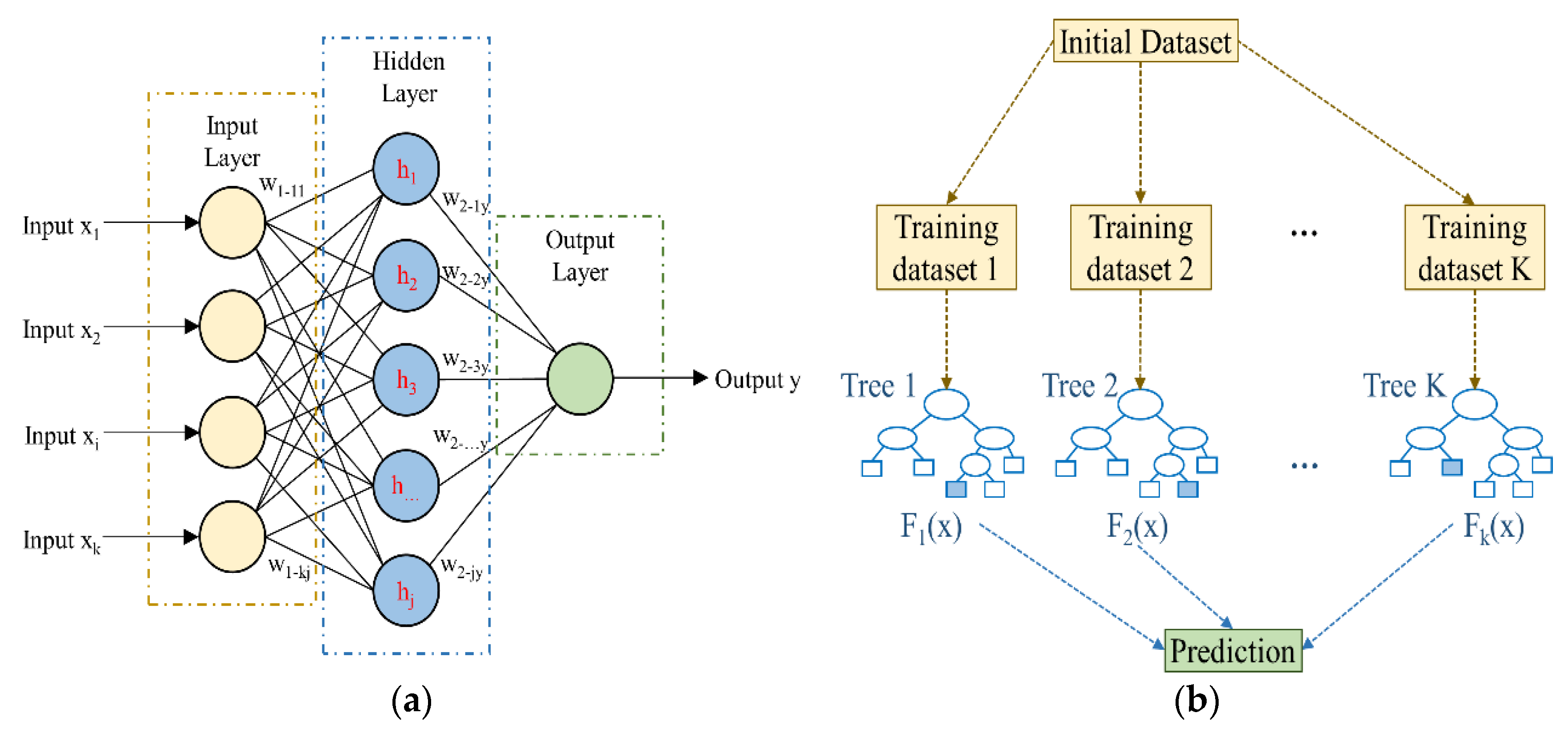
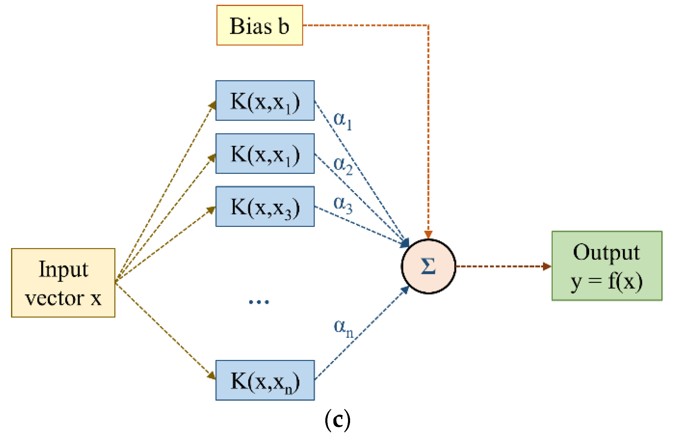
2.1. Standalone Machine Learning Algorithms
2.2. Evaluation Criteria
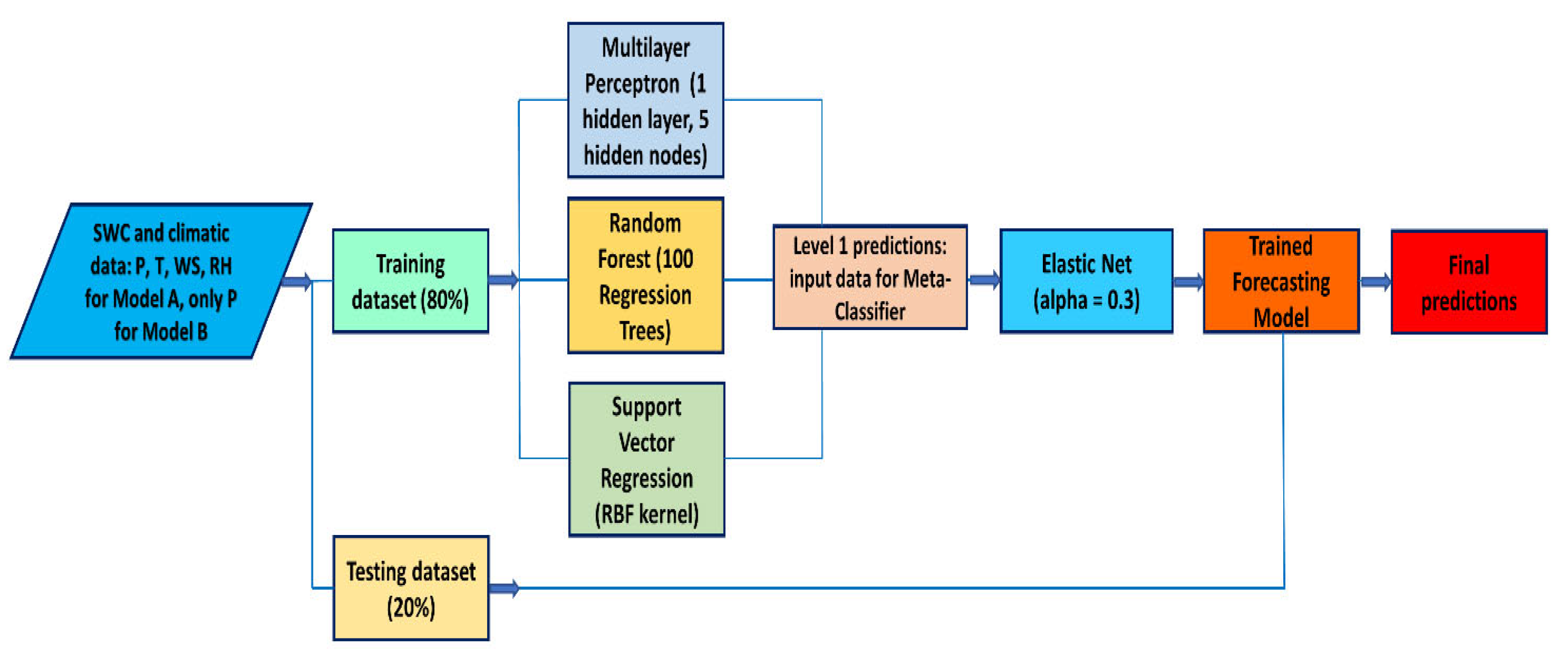
2.3. Stacked Model Development

| Algorithm | Hyperparameter | Value |
|---|---|---|
| MLP | Number of hidden layers | 1 |
| Number of hidden neurons | 5 | |
| Activation function | Sigmoid | |
| RF | Number of trees | 100 |
| SVR | Kernel function | RBF |
| C | 2 | |
| ε | 0.01 | |
| EN | α | 0.3 |
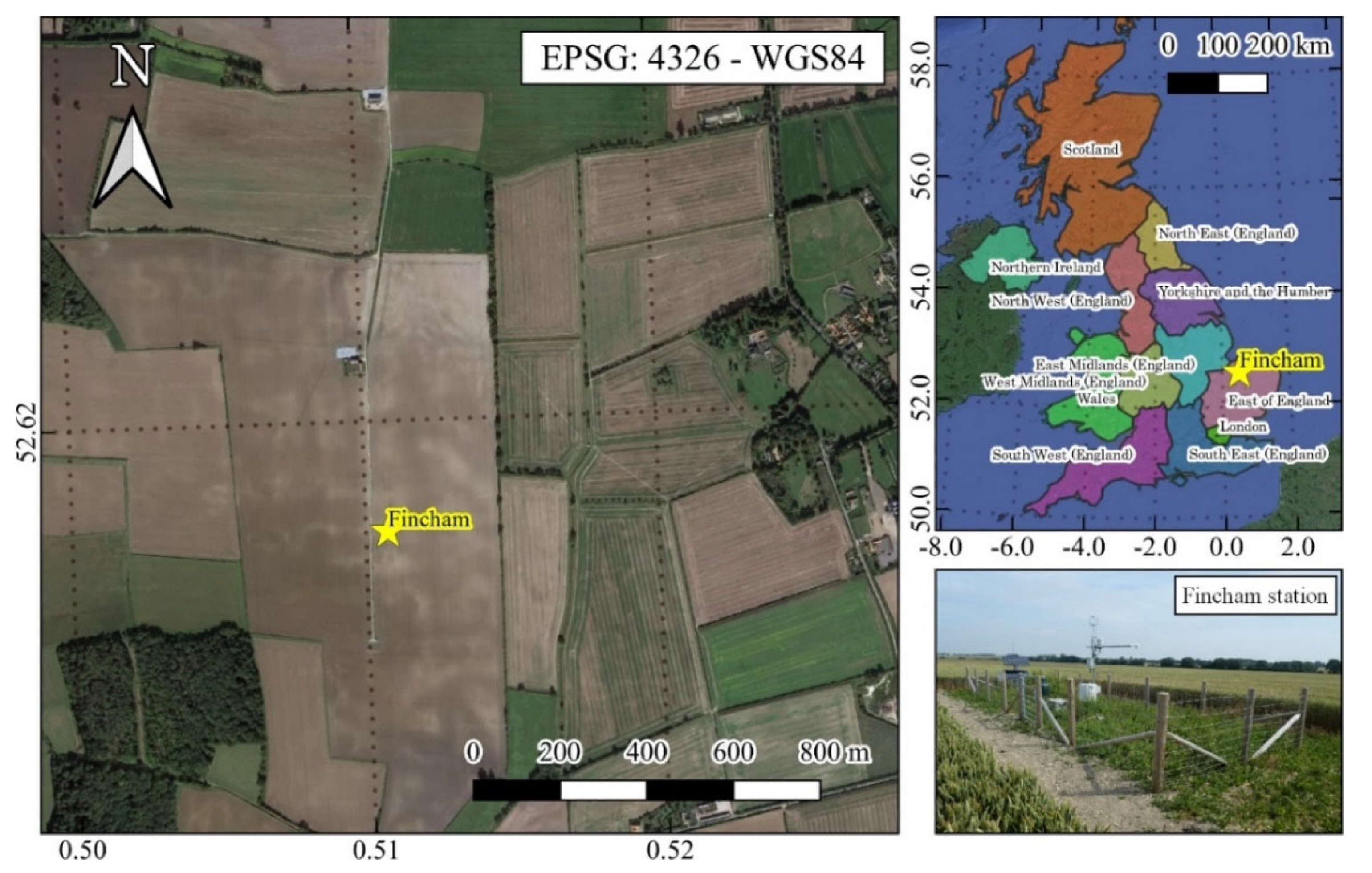
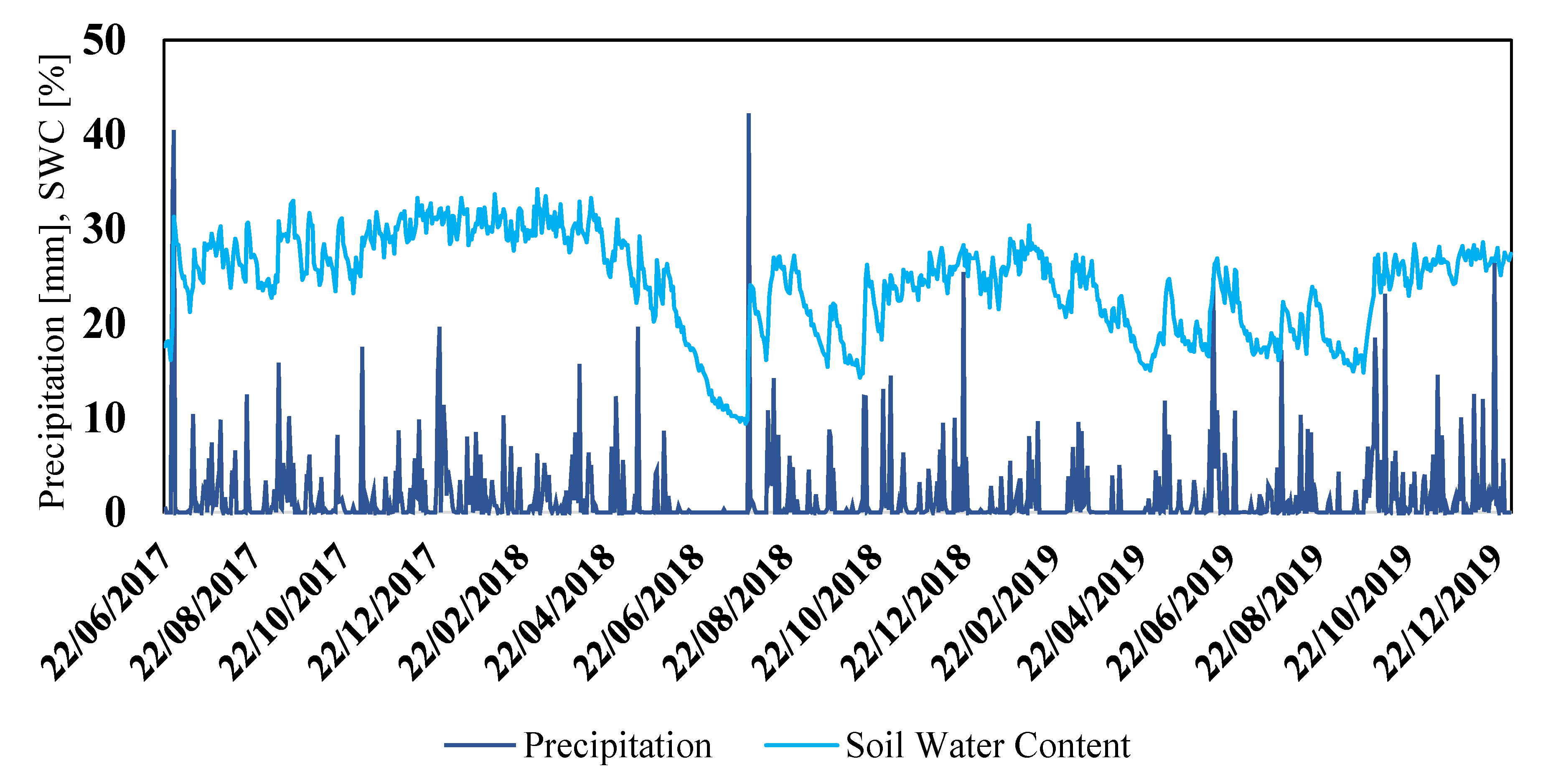
2.4. Case Study
3. Results
4. Discussion
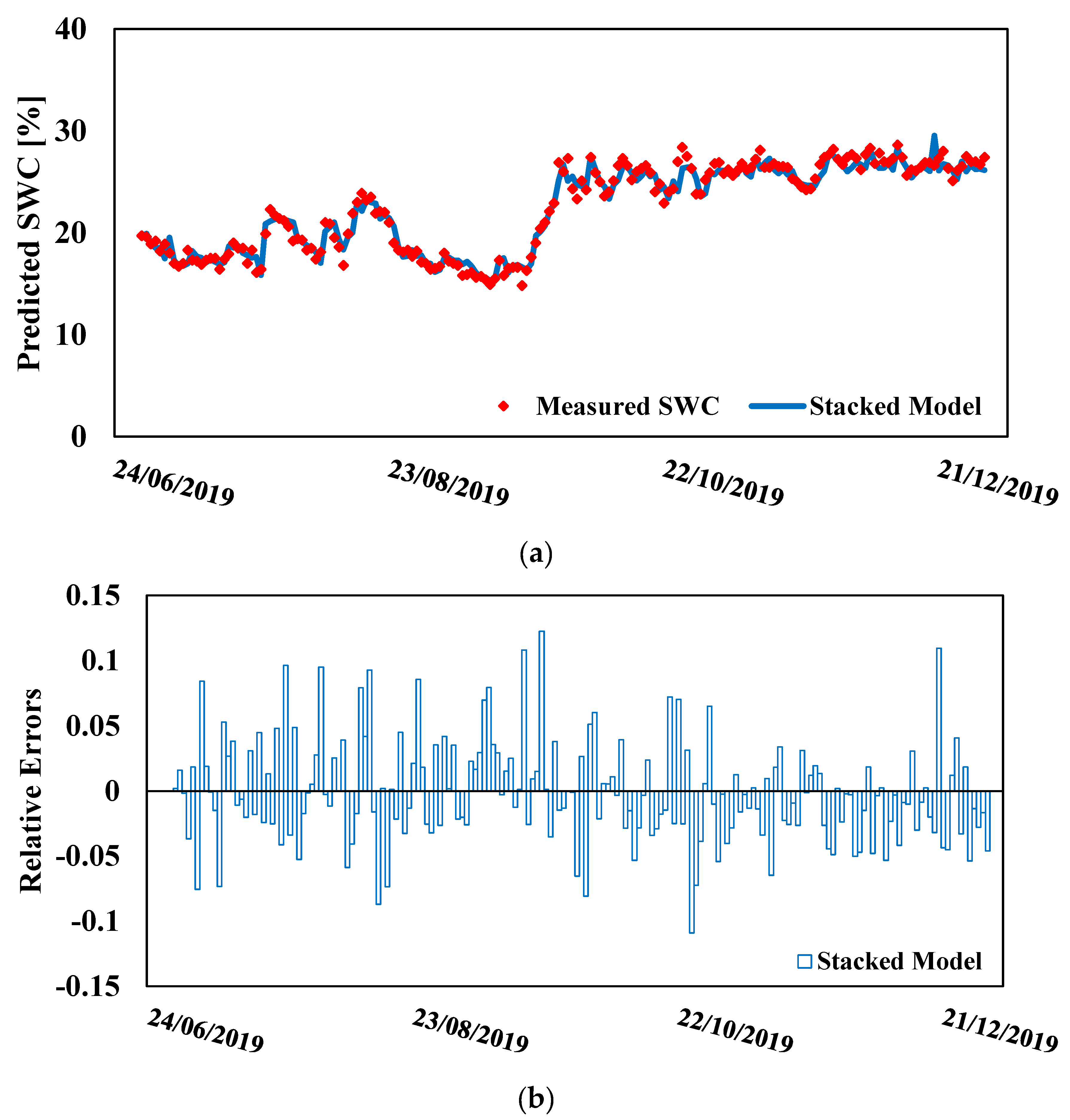
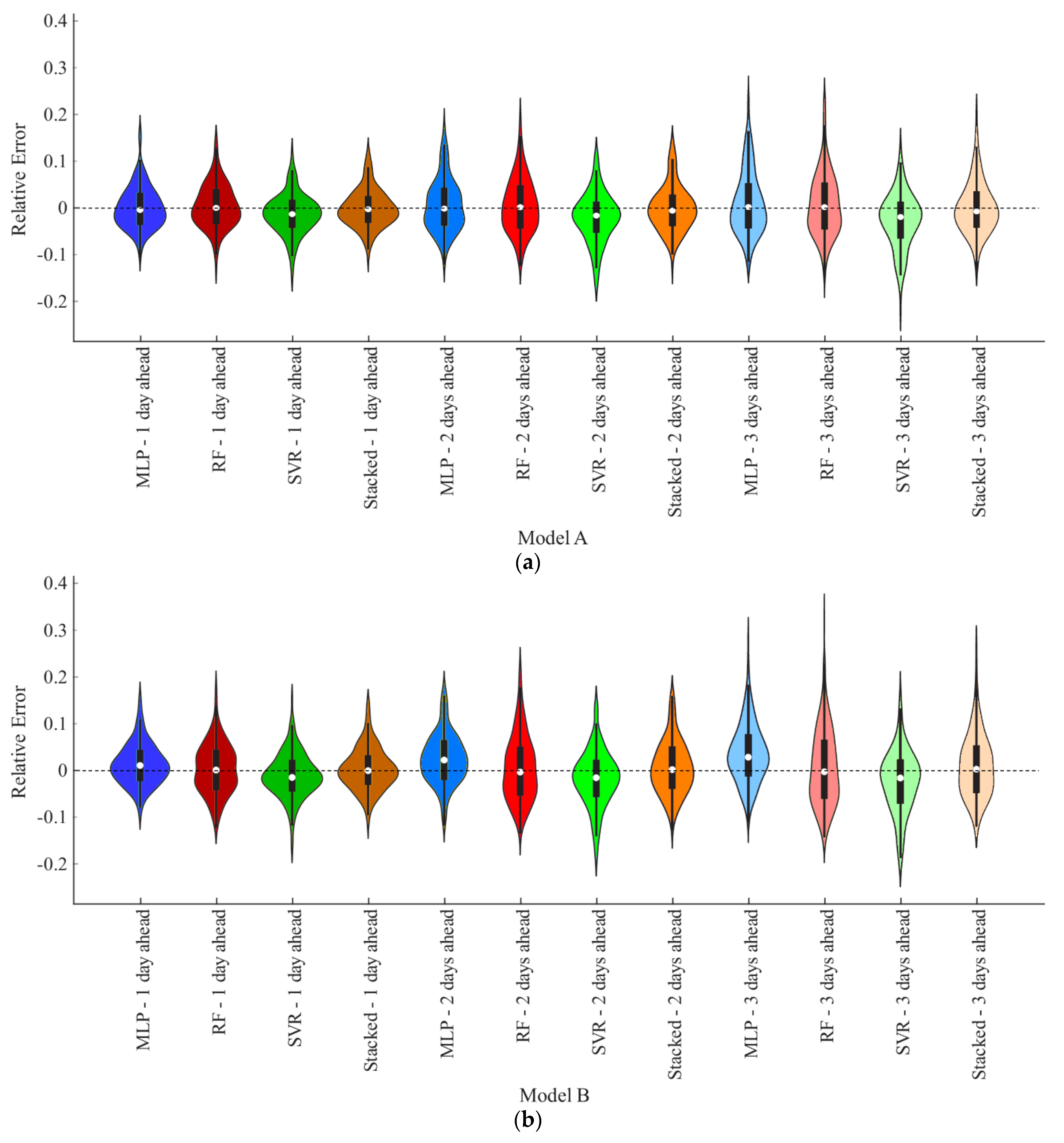
- In the case of Model A, only the SVR-based variant was characterized by an appreciable bias, whereas in the case of Model B, an appreciable bias could be found in both the MLP- and SVR-based variants.
- The distribution of the relative error in both models was asymmetrical in many cases.
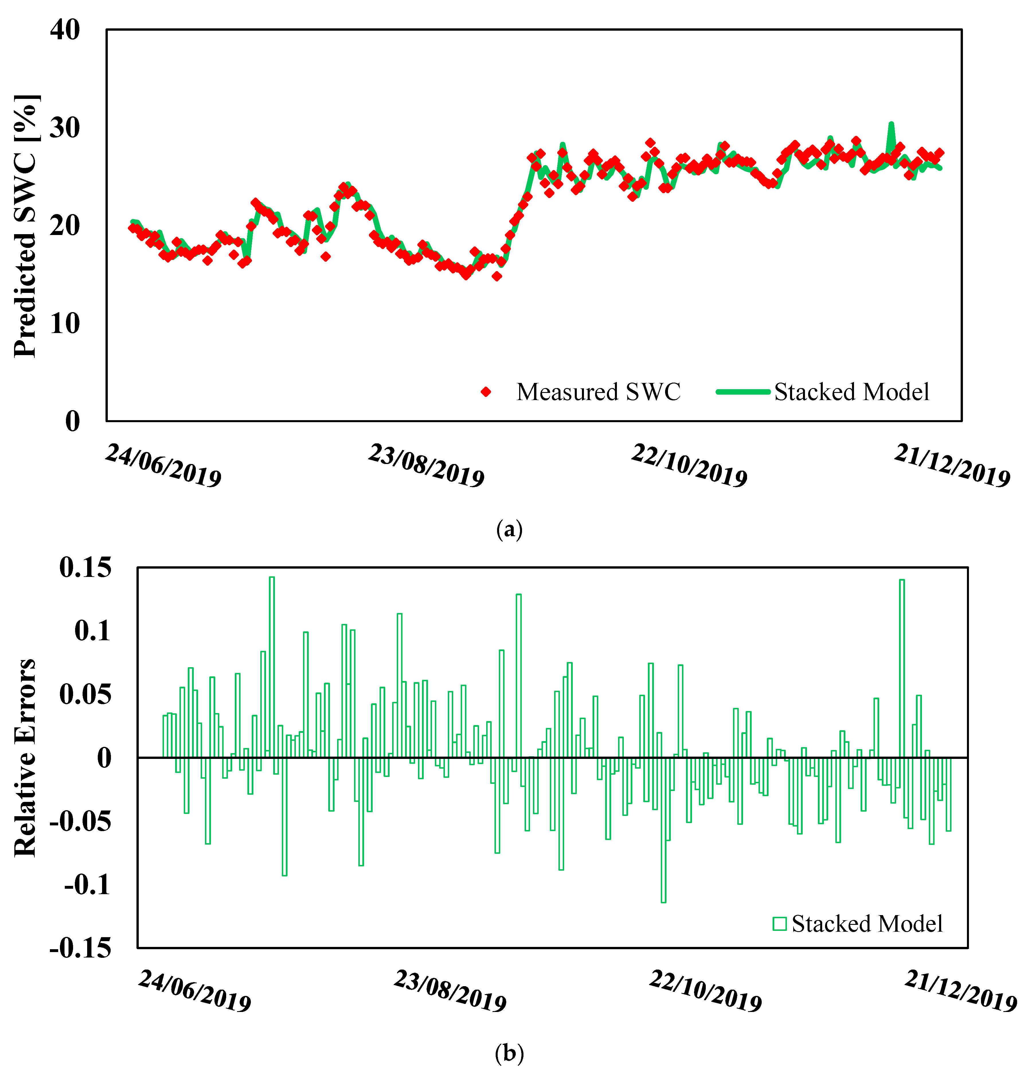
- The error distribution tended to become flatter as the forecast horizon increased, and the IQR of the relative error expanded as the forecast horizon increased. The standard deviation of the residuals increased as the forecasting horizon increased. For example, with reference to Model A based on the SM, it was 0.874, 1.049, and 1.164% for the 1-day-ahead, 2-days-ahead, and 3-days-ahead forecasts, respectively. With reference to the SM-based Model B, the standard deviation of the residuals was 0.978, 1.227, and 1.414 for the 1-day-ahead, 2-days-ahead, and 3-days-ahead forecasts, respectively.
- The number of outliers resulting from forecasting models was very low.
5. Conclusions
Author Contributions
Funding
Data Availability Statement
Conflicts of Interest
References
- Seneviratne, S.I.; Corti, T.; Davin, E.L.; Hirschi, M.; Jaeger, E.B.; Lehner, I.; Orlowsky, B.; Teuling, A.J. Investigating soil moisture–climate interactions in a changing climate: A review. Earth-Sci. Rev. 2010, 99, 125–161. [Google Scholar] [CrossRef]
- Sit, M.; Demir, I. Decentralized flood forecasting using deep neural networks. arXiv 2019, arXiv:1902.02308. [Google Scholar]
- Walker, J.P.; Willgoose, G.R.; Kalma, J.D. In situ measurement of soil moisture: A comparison of techniques. J. Hydrol. 2004, 293, 85–99. [Google Scholar] [CrossRef]
- Demir, I.; Conover, H.; Krajewski, W.F.; Seo, B.C.; Goska, R.; He, Y.; McEniry, M.F.; Graves, S.J.; Petersen, W. Data-enabled field experiment planning, management, and research using cyberinfrastructure. J. Hydrometeorol. 2015, 16, 1155–1170. [Google Scholar] [CrossRef]
- Mohanty, B.P.; Cosh, M.H.; Lakshmi, V.; Montzka, C. Soil moisture remote sensing: State-of-the-science. Vadose Zone J. 2017, 16, 1–9. [Google Scholar] [CrossRef] [Green Version]
- Yildirim, E.; Demir, I. Agricultural flood vulnerability assessment and risk quantification in Iowa. Sci. Total Environ. 2022, 826, 154165. [Google Scholar] [CrossRef]
- Brocca, L.; Ciabatta, L.; Massari, C.; Camici, S.; Tarpanelli, A. Soil moisture for hydrological applications: Open questions and new opportunities. Water 2017, 9, 140. [Google Scholar] [CrossRef]
- Soulis, K.X.; Elmaloglou, S.; Dercas, N. Investigating the effects of soil moisture sensors positioning and accuracy on soil moisture based drip irrigation scheduling systems. Agric. Water Manag. 2015, 148, 258–268. [Google Scholar] [CrossRef]
- Kişi, Ö. Streamflow forecasting using different artificial neural network algorithms. J. Hydrol. Eng. 2007, 12, 532–539. [Google Scholar] [CrossRef]
- Nourani, V.; Kisi, Ö.; Komasi, M. Two hybrid artificial intelligence approaches for modeling rainfall–runoff process. J. Hydrol. 2011, 402, 41–59. [Google Scholar] [CrossRef]
- Granata, F. Evapotranspiration evaluation models based on machine learning algorithms—A comparative study. Agric. Water Manag. 2019, 217, 303–315. [Google Scholar] [CrossRef]
- Di Nunno, F.; Granata, F. Groundwater level prediction in Apulia region (Southern Italy) using NARX neural network. Environ. Res. 2020, 190, 110062. [Google Scholar] [CrossRef] [PubMed]
- Xiang, Z.; Demir, I. Distributed long-term hourly streamflow predictions using deep learning—A case study for State of Iowa. Environ. Model. Softw. 2020, 131, 104761. [Google Scholar] [CrossRef]
- Granata, F.; Di Nunno, F. Forecasting evapotranspiration in different climates using ensembles of recurrent neural networks. Agric. Water Manag. 2021, 255, 107040. [Google Scholar] [CrossRef]
- Granata, F.; Di Nunno, F.; Modoni, G. Hybrid Machine Learning Models for Soil Saturated Conductivity Prediction. Water 2022, 14, 1729. [Google Scholar] [CrossRef]
- Rozos, E.; Leandro, J.; Koutsoyiannis, D. Development of Rating Curves: Machine Learning vs. Statistical Methods. Hydrology 2022, 9, 166. [Google Scholar] [CrossRef]
- Rozos, E.; Koutsoyiannis, D.; Montanari, A. KNN vs. Bluecat—Machine Learning vs. Classical Statistics. Hydrology 2022, 9, 101. [Google Scholar] [CrossRef]
- Elshorbagy, A.; Parasuraman, K. On the relevance of using artificial neural networks for estimating soil moisture content. J. Hydrol. 2008, 362, 1–18. [Google Scholar] [CrossRef]
- Si, J.; Feng, Q.; Wen, X.; Xi, H.; Yu, T.; Li, W.; Zhao, C. Modeling soil water content in extreme arid area using an adaptive neuro-fuzzy inference system. J. Hydrol. 2015, 527, 679–687. [Google Scholar] [CrossRef]
- Zanetti, S.S.; Cecílio, R.A.; Silva, V.H.; Alves, E.G. General calibration of TDR to assess the moisture of tropical soils using artificial neural networks. J. Hydrol. 2015, 530, 657–666. [Google Scholar] [CrossRef]
- Cui, Y.; Long, D.; Hong, Y.; Zeng, C.; Zhou, J.; Han, Z.; Liu, R.; Wan, W. Validation and reconstruction of FY-3B/MWRI soil moisture using an artificial neural network based on reconstructed MODIS optical products over the Tibetan Plateau. J. Hydrol. 2016, 543, 242–254. [Google Scholar] [CrossRef]
- Prasad, R.; Deo, R.C.; Li, Y.; Maraseni, T. Soil moisture forecasting by a hybrid machine learning technique: ELM integrated with ensemble empirical mode decomposition. Geoderma 2018, 330, 136–161. [Google Scholar] [CrossRef]
- Prasad, R.; Deo, R.C.; Li, Y.; Maraseni, T. Ensemble committee-based data intelligent approach for generating soil moisture forecasts with multivariate hydro-meteorological predictors. Soil Tillage Res. 2018, 181, 63–81. [Google Scholar] [CrossRef]
- Prasad, R.; Deo, R.C.; Li, Y.; Maraseni, T. Weekly soil moisture forecasting with multivariate sequential, ensemble empirical mode decomposition and Boruta-random forest hybridizer algorithm approach. Catena 2019, 177, 149–166. [Google Scholar] [CrossRef]
- Maroufpoor, S.; Maroufpoor, E.; Bozorg-Haddad, O.; Shiri, J.; Yaseen, Z.M. Soil moisture simulation using hybrid artificial intelligent model: Hybridization of adaptive neuro fuzzy inference system with grey wolf optimizer algorithm. J. Hydrol. 2019, 575, 544–556. [Google Scholar] [CrossRef]
- Achieng, K.O. Modelling of soil moisture retention curve using machine learning techniques: Artificial and deep neural networks vs support vector regression models. Comput. Geosci. 2019, 133, 104320. [Google Scholar] [CrossRef]
- Yuan, Q.; Xu, H.; Li, T.; Shen, H.; Zhang, L. Estimating surface soil moisture from satellite observations using a generalized regression neural network trained on sparse ground-based measurements in the continental US. J. Hydrol. 2020, 580, 124351. [Google Scholar] [CrossRef]
- Heddam, S. New formulation for predicting soil moisture content using only soil temperature as predictor: Multivariate adaptive regression splines versus random forest, multilayer perceptron neural network, M5Tree, and multiple linear regression. In Water Engineering Modeling and Mathematic Tools; Elsevier: Amsterdam, The Netherlands, 2021; pp. 45–62. [Google Scholar]
- Liu, H.; Xie, D.; Wu, W. Soil water content forecasting by ANN and SVM hybrid architecture. Environ. Monit. Assess. 2008, 143, 187–193. [Google Scholar] [CrossRef]
- Ahmad, S.; Kalra, A.; Stephen, H. Estimating soil moisture using remote sensing data: A machine learning approach. Adv. Water Resour. 2010, 33, 69–80. [Google Scholar] [CrossRef]
- Karandish, F.; Šimůnek, J. A comparison of numerical and machine-learning modeling of soil water content with limited input data. J. Hydrol. 2016, 543, 892–909. [Google Scholar] [CrossRef] [Green Version]
- Cai, Y.; Zheng, W.; Zhang, X.; Zhangzhong, L.; Xue, X. Research on soil moisture prediction model based on deep learning. PLoS ONE 2019, 14, e0214508. [Google Scholar] [CrossRef] [PubMed]
- Adab, H.; Morbidelli, R.; Saltalippi, C.; Moradian, M.; Ghalhari, G.A.F. Machine learning to estimate surface soil moisture from remote sensing data. Water 2020, 12, 3223. [Google Scholar] [CrossRef]
- Granata, F.; Di Nunno, F.; de Marinis, G. Stacked machine learning algorithms and bidirectional long short-term memory networks for multi-step ahead streamflow forecasting: A comparative study. J. Hydrol. 2022, 613, 128431. [Google Scholar] [CrossRef]
- Rosenblatt, F. Principles of Neurodynamics. Perceptrons and the Theory of Brain Mechanisms; Cornell Aeronautical Lab Inc.: Buffalo, NY, USA, 1961. [Google Scholar]
- Murtagh, F. Multilayer perceptrons for classification and regression. Neurocomputing 1991, 2, 183–197. [Google Scholar] [CrossRef]
- Breiman, L. Random forests. Mach. Learn. 2001, 45, 5–32. [Google Scholar] [CrossRef] [Green Version]
- Breiman, L.; Friedman, J.H.; Olshen, R.A.; Stone, C.J. Classification and Regression Trees; Routledge: Oxford, UK, 2017. [Google Scholar]
- Cortes, C.; Vapnik, V. Support-vector networks. Mach. Learn. 1995, 20, 273–297. [Google Scholar] [CrossRef]
- Wolpert, D.H. Stacked generalization. Neural Netw. 1992, 5, 241–259. [Google Scholar] [CrossRef]
- Breiman, L. Stacked regressions. Mach. Learn. 1996, 24, 49–64. [Google Scholar] [CrossRef] [Green Version]
- Zou, H.; Hastie, T. Regularization and variable selection via the elastic net. J. R. Stat. Soc. Ser. B Stat. Methodol. 2005, 67, 301–320. [Google Scholar] [CrossRef] [Green Version]
- Zreda, M.; Desilets, D.; Ferré, T.P.A.; Scott, R.L. Measuring soil moisture content non-invasively at intermediate spatial scale using cosmic-ray neutrons. Geophys. Res. Lett. 2008, 35, L21402. [Google Scholar] [CrossRef] [Green Version]
- Desilets, D.; Zreda, M.; Ferré, T.P. Nature’s neutron probe: Land surface hydrology at an elusive scale with cosmic rays. Water Resour. Res. 2010, 46. [Google Scholar] [CrossRef]
- Andreasen, M.; Jensen, K.H.; Zreda, M.; Desilets, D.; Bogena, H.; Looms, M.C. Modeling cosmic ray neutron field measurements. Water Resour. Res. 2016, 52, 6451–6471. [Google Scholar] [CrossRef] [Green Version]
- Box, G.E.P.; Jenkins, G.M. Some recent advances in forecasting and control. J. R. Stat. Soc. Ser. C Appl. Stat. 1968, 17, 91–109. [Google Scholar] [CrossRef]
- Fan, J.; Shan, R.; Cao, X. The analysis to Tertiary-industry with ARIMAX model. J. Math. Res. 2009, 1, 156–163. [Google Scholar] [CrossRef] [Green Version]
- Demir, I.; Xiang, Z.; Demiray, B.; Sit, M. WaterBench: A Large-scale Benchmark Dataset for Data-Driven Streamflow Forecasting. Earth Syst. Sci. Data Discuss. 2022, 14, 1–19. [Google Scholar] [CrossRef]
- Das, B.; Rathore, P.; Roy, D.; Chakraborty, D.; Jatav, R.S.; Sethi, D.; Kumar, P. Comparison of bagging, boosting and stacking algorithms for surface soil moisture mapping using optical-thermal-microwave remote sensing synergies. Catena 2022, 217, 106485. [Google Scholar] [CrossRef]
- Sit, M.; Demiray, B.Z.; Xiang, Z.; Ewing, G.J.; Sermet, Y.; Demir, I. A comprehensive review of deep learning applications in hydrology and water resources. Water Sci. Technol. 2020, 82, 2635–2670. [Google Scholar] [CrossRef]
- Di Nunno, F.; de Marinis, G.; Gargano, R.; Granata, F. Tide prediction in the Venice Lagoon using nonlinear autoregressive exogenous (NARX) neural network. Water 2021, 13, 1173. [Google Scholar] [CrossRef]
- Yildirim, E.; Demir, I. An integrated flood risk assessment and mitigation framework: A case study for middle Cedar River Basin, Iowa, US. Int. J. Disaster Risk Reduct. 2021, 56, 102113. [Google Scholar] [CrossRef]


| SWC [%] | Air Temp. [°C] | Wind Speed [m/s] | Rel. Hum. [%] | |
|---|---|---|---|---|
| Mean | 24.18 | 11.06 | 3.28 | 80.12 |
| Median | 25.00 | 11.12 | 3.03 | 81.43 |
| Max | 34.20 | 27.36 | 8.52 | 99.62 |
| Min | 9.40 | −4.82 | 0.67 | 53.36 |
| St. Deviation | 5.16 | 5.54 | 1.42 | 9.50 |
| CV | 0.21 | 0.50 | 0.43 | 0.12 |
| 1st Quartile | 20.55 | 6.79 | 2.20 | 73.00 |
| 3rd Quartile | 27.90 | 15.50 | 4.14 | 87.82 |
| Skewness | −0.57 | 0.00 | 0.88 | −0.31 |
| MLP | RF | SVR | Stacked Model | |||
|---|---|---|---|---|---|---|
| Model A (Training) | 1-day-ahead | R2 | 0.957 | 0.992 | 0.942 | 0.968 |
| RMSE | 1.092 | 0.49 | 1.267 | 0.937 | ||
| MAE | 0.816 | 0.356 | 0.911 | 0.694 | ||
| MAPE | 3.36% | 1.49% | 3.73% | 2.85% | ||
| 2-days-ahead | R2 | 0.940 | 0.985 | 0.912 | 0.953 | |
| RMSE | 1.285 | 0.663 | 1.569 | 1.137 | ||
| MAE | 1.009 | 0.469 | 1.139 | 0.861 | ||
| MAPE | 4.22% | 1.94% | 4.68% | 3.56% | ||
| 3-days-ahead | R2 | 0.928 | 0.977 | 0.891 | 0.941 | |
| RMSE | 1.406 | 0.829 | 1.752 | 1.276 | ||
| MAE | 1.101 | 0.571 | 1.266 | 0.959 | ||
| MAPE | 4.66% | 2.36% | 5.24% | 3.99% | ||
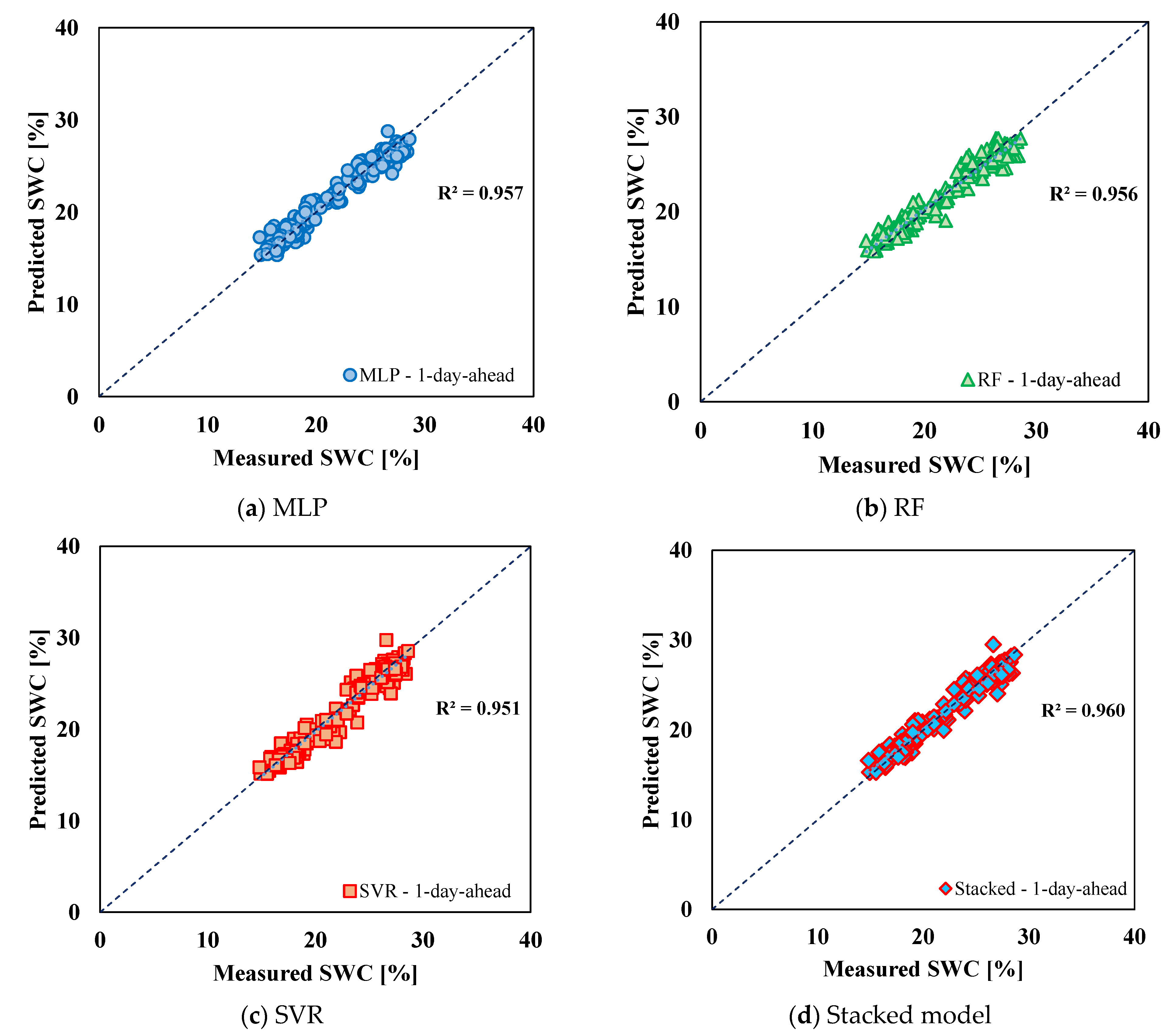
| Model A (Testing) | 1-day-ahead | R2 | 0.957 | 0.956 | 0.951 | 0.962 |
| RMSE | 0.924 | 0.985 | 0.996 | 0.877 | ||
| MAE | 0.741 | 0.787 | 0.744 | 0.673 | ||
| MAPE | 3.41% | 3.62% | 3.35% | 3.05% | ||
| 2-days-ahead | R2 | 0.940 | 0.938 | 0.927 | 0.946 | |
| RMSE | 1.146 | 1.217 | 1.264 | 1.053 | ||
| MAE | 0.942 | 0.990 | 0.945 | 0.821 | ||
| MAPE | 4.40% | 4.59% | 4.27% | 3.74% | ||
| 3-days-ahead | R2 | 0.921 | 0.929 | 0.911 | 0.935 | |
| RMSE | 1.355 | 1.360 | 1.442 | 1.169 | ||
| MAE | 1.105 | 1.113 | 1.069 | 0.921 | ||
| MAPE | 5.25% | 5.22% | 4.83% | 4.22% |
| MLP | RF | SVR | Stacked Model | |||
|---|---|---|---|---|---|---|
| Model B (Training) | 1-day-ahead | R2 | 0.946 | 0.990 | 0.934 | 0.965 |
| RMSE | 1.222 | 0.533 | 1.365 | 0.989 | ||
| MAE | 0.914 | 0.394 | 0.979 | 0.737 | ||
| MAPE | 3.72% | 1.62% | 3.94% | 3.02% | ||
| 2-days-ahead | R2 | 0.919 | 0.976 | 0.892 | 0.943 | |
| RMSE | 1.495 | 0.835 | 1.749 | 1.258 | ||
| MAE | 1.161 | 0.586 | 1.274 | 0.964 | ||
| MAPE | 4.77% | 2.38% | 5.13% | 3.98% | ||
| 3-days-ahead | R2 | 0.900 | 0.960 | 0.863 | 0.925 | |
| RMSE | 1.658 | 1.073 | 1.989 | 1.441 | ||
| MAE | 1.286 | 0.745 | 1.479 | 1.109 | ||
| MAPE | 5.32% | 3.01% | 5.98% | 4.62% | ||
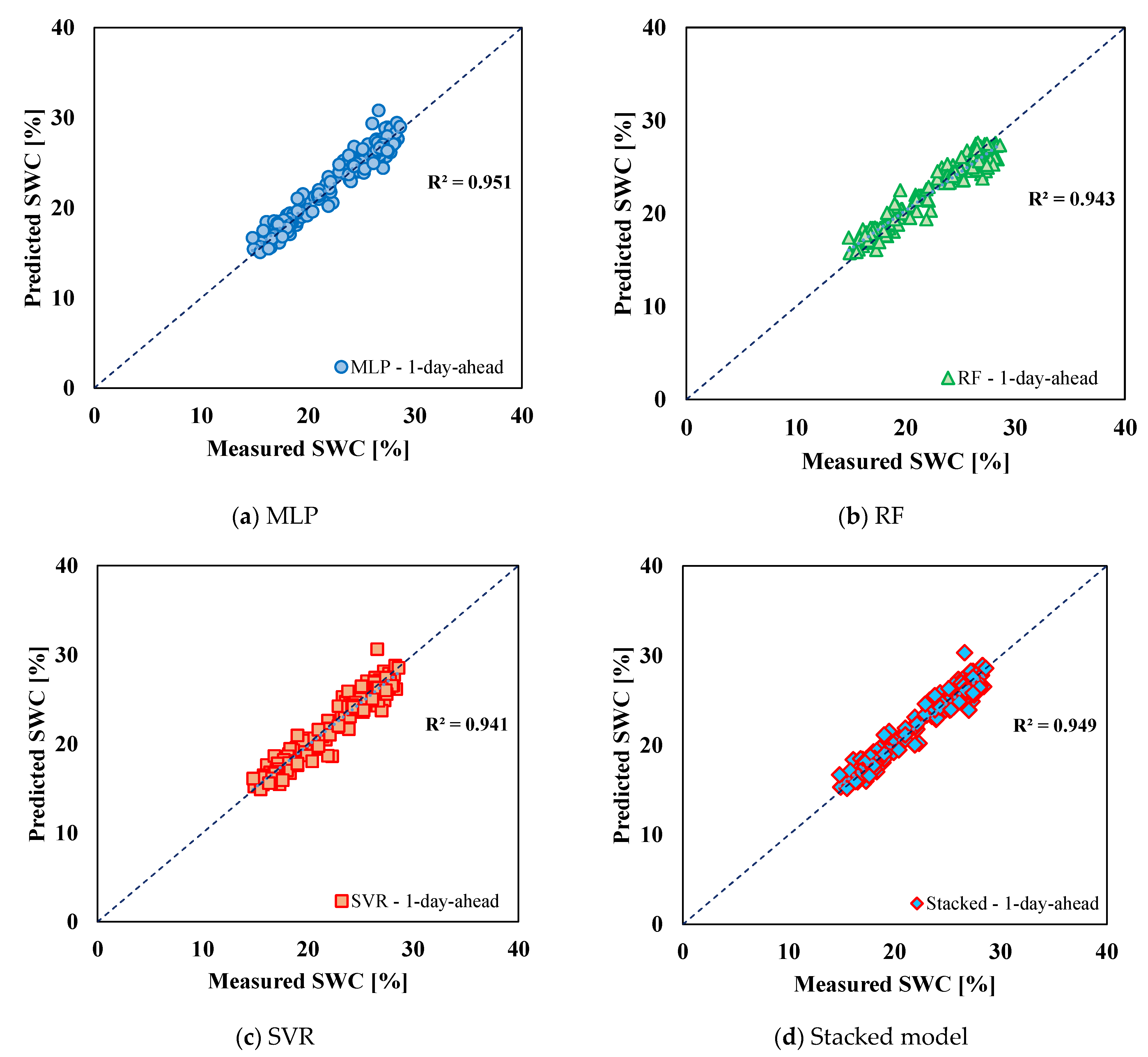
| Model B (Testing) | 1-day-ahead | R2 | 0.951 | 0.943 | 0.941 | 0.949 |
| RMSE | 0.982 | 1.145 | 1.069 | 0.976 | ||
| MAE | 0.745 | 0.937 | 0.810 | 0.751 | ||
| MAPE | 3.42% | 4.28% | 3.64% | 3.39% | ||
| 2-days-ahead | R2 | 0.928 | 0.916 | 0.907 | 0.924 | |
| RMSE | 1.249 | 1.456 | 1.381 | 1.224 | ||
| MAE | 0.964 | 1.198 | 1.028 | 0.973 | ||
| MAPE | 4.48% | 5.53% | 4.59% | 4.45% | ||
| 3-days-ahead | R2 | 0.903 | 0.896 | 0.880 | 0.902 | |
| RMSE | 1.513 | 1.667 | 1.606 | 1.411 | ||
| MAE | 1.185 | 1.381 | 1.193 | 1.144 | ||
| MAPE | 5.56% | 6.43% | 5.32% | 5.29% |
| ARIMAX | ||
|---|---|---|
| 1-day-ahead | R2 | 0.944 |
| RMSE | 1.046 | |
| MAE | 0.831 | |
| MAPE | 3.88% | |
| 2-days-ahead | R2 | 0.924 |
| RMSE | 1.284 | |
| MAE | 0.997 | |
| MAPE | 5.23% | |
| 3-days-ahead | R2 | 0.910 |
| RMSE | 1.542 | |
| MAE | 1.124 | |
| MAPE | 5.63% | |
Disclaimer/Publisher’s Note: The statements, opinions and data contained in all publications are solely those of the individual author(s) and contributor(s) and not of MDPI and/or the editor(s). MDPI and/or the editor(s) disclaim responsibility for any injury to people or property resulting from any ideas, methods, instructions or products referred to in the content. |
© 2022 by the authors. Licensee MDPI, Basel, Switzerland. This article is an open access article distributed under the terms and conditions of the Creative Commons Attribution (CC BY) license (https://creativecommons.org/licenses/by/4.0/).
Share and Cite
Granata, F.; Di Nunno, F.; Najafzadeh, M.; Demir, I. A Stacked Machine Learning Algorithm for Multi-Step Ahead Prediction of Soil Moisture. Hydrology 2023, 10, 1. https://doi.org/10.3390/hydrology10010001
Granata F, Di Nunno F, Najafzadeh M, Demir I. A Stacked Machine Learning Algorithm for Multi-Step Ahead Prediction of Soil Moisture. Hydrology. 2023; 10(1):1. https://doi.org/10.3390/hydrology10010001
Chicago/Turabian StyleGranata, Francesco, Fabio Di Nunno, Mohammad Najafzadeh, and Ibrahim Demir. 2023. "A Stacked Machine Learning Algorithm for Multi-Step Ahead Prediction of Soil Moisture" Hydrology 10, no. 1: 1. https://doi.org/10.3390/hydrology10010001