Article

Exploring Temporal Dynamics of River Discharge Using Univariate Long Short-Term Memory (LSTM) Recurrent Neural Network at East Branch of Delaware River

by
Md Abdullah Al Mehedi
1,
Marzieh Khosravi
1,*,
Munshi Md Shafwat Yazdan
2 and
Hanieh Shabanian
3
1
College of Engineering, Villanova University, Villanova, PA 19085, USA
2
Civil and Environmental Engineering, Idaho State University, Pocatello, ID 83209, USA
3
Department of Computer Science, Northern Kentucky University, Highland Heights, KY 41099, USA
*
Author to whom correspondence should be addressed.
Hydrology 2022, 9(11), 202; https://doi.org/10.3390/hydrology9110202
Submission received: 8 September 2022 / Revised: 7 November 2022 / Accepted: 8 November 2022 / Published: 11 November 2022

Abstract

:
River flow prediction is a pivotal task in the field of water resource management during the era of rapid climate change. The highly dynamic and evolving nature of the climatic variables, e.g., precipitation, has a significant impact on the temporal distribution of the river discharge in recent days, making the discharge forecasting even more complicated for diversified water-related issues, e.g., flood prediction and irrigation planning. In order to predict the discharge, various physics-based numerical models are used using numerous hydrologic parameters. Extensive lab-based investigation and calibration are required to reduce the uncertainty involved in those parameters. However, in the age of data-driven predictions, several deep learning algorithms showed satisfactory performance in dealing with sequential data. In this research, Long Short-term Memory (LSTM) neural network regression model is trained using over 80 years of daily data to forecast the discharge time series up to seven days ahead of time. The performance of the model is found satisfactory through the comparison of the predicted data with the observed data, visualization of the distribution of the errors, and R2 value of 0.93 with one day lead time. Higher performance is achieved through the increase in the number of epochs and hyperparameter tuning. This model can be transferred to other locations with proper feature engineering and optimization to perform univariate predictive analysis and potentially be used to perform real-time river discharge prediction.

1. Introduction

River discharge forecasting is considered a pivotal task in various fields of water resource management, i.e., flood control, irrigation planning, and hydropower production [1,2,3,4,5,6,7]. River discharge has a significant impact on the physical, chemical and biological activities in the river contributing high correlation to the fluvial ecosystem [8,9,10,11]. Various methods of forecasting are established on the probability of future river flow using historical data or records. Forecasting models using Deep Learning algorithms (e.g., short-term and long-term forecasting models) have a significant interest in the research and scientific community [12,13,14,15]. Due to the complexity, climate changeability, and effects on anthropology, hydrological data holds a strong constraint to the advancement of short-term forecasting models [16,17,18,19]. Methodologies for river discharge modeling and forecasting can be divided into three groups: conceptual, physics-based, and data-driven models [20]. A lot of research has already been conducted with a focus on the use of conceptual and physics-based models [21,22]. For modeling streamflow, simple conceptual R-R models are widely employed since they often provide reasonable prediction accuracy [23]. In addition, several pieces of research demonstrate that conceptual and physics-based models have a limited competence to provide short-term forecasts and require long-term datasets to perform the computationally expensive model calibration [24]. Furthermore, some studies show that conceptual and physics-based models, in some circumstances, showed limited capability in flood forecasting in higher dimensions [25]. In the last decade, many scientists and researchers have examined the pros and cons of various conceptual and physics-based models and have compared their prediction performance with that of emerging data-driven techniques, e.g., Deep Learning (DL) methods [11,26]. Recently, the practice of data-driven techniques of DL methods has drawn substantial consideration for the sequential data, e.g., precipitation and river flow prediction applications. Scientists from all over the world have concluded that data-driven techniques of DL methods are qualified to capture non-linear processes numerically without the knowledge of the underlying conceptual or physical processes involved [27,28,29,30].
This study is a valuable contribution to river discharge prediction using the DL method, which contributes to understanding the dynamics of river flow and offers a framework to predict the impact of it on agriculture, fluvial ecology, flooding, irrigation, and water supply planning in the nearby areas. The proposed methodology is applied to the East Branch of Delaware River in Delaware County, NY, because there is an eighty-year-long record of daily flows available.
Data-driven techniques can be divided into two methods, such as statistical methods and black-box models. Statistical models deal with autoregressive Moving Average (MA) techniques [31,32]. On the other hand, the black box models follow various techniques of Artificial Intelligence (AI) [33]. The Machine Learning (ML) methods to make the river discharge prediction consist of Artificial Neural Networks (ANN) [34,35,36,37,38,39,40], Support Vector Regression (SVR) [41,42,43,44,45], Decision Tree (DT) model [46,47], fuzzy inference system [48], Bayesian particle filter [49], expert system [50], hybrid model [51], and Multiple Linear Regression (MLR) [52]. The spatial and temporal hidden patterns in historical data are explored by these ML/DL methods without using a conceptual or even physical model, as it requires a large number of physical parameters and a broad understanding of the physical processes in the domain of the model [53]. In many cases, streamflow analysis using ANN can accomplish a better and accurate predictive performance than conceptual or physically based models [54]. However, the traditional ANN algorithms e.g., Feed Forward Neural Network (FFNN) do not have the ability to learn sequential data as they cannot recall previous information flow, resulting in a constrained prediction capability for long-term time series, e.g., temporal distribution of the discharge/water depth. The FFNN algorithms need complex procedures in the data pre-processing stage to obtain good performance in predicting the target variables. While comprehensive data pre-processing can bolster the ability of a FFNN model to learn from the observed data, it requires a significant amount of user intervention, e.g., selecting the number of reconstructed components38. In addition, the pre-processing requires a substantial amount of time as many reconstructed components need to be calculated.
In contrast, an updated version of Recurrent Neural Network (RNN), Long Short-Term Memory (LSTM), has achieved significant attention among the water scientist community, specifically for time series prediction. LSTM was first introduced by Hochreiter and Schmidhuber in 1997 and has later been established as a powerful tool for addressing forecasting problems [55,56,57,58,59,60]. High computational effort and time are needed by recurrent backpropagation to learn to store long-term information because of the decaying error backflow. Hence, the concept of the vanishing gradient problem in recognizing the long-term dependency of RNN was introduced [61]. LSTM has become a very popular algorithm to deal with time series data in DL forecasting, where variables are dependent on the previous information along the series. LSTM can capture the long-term dependencies and linkage among the variables. Compared to traditional neural networks, e.g., FFNN, LSTMs are capable of capturing both the Chaotic and periodic behaviors of time series data and determining the dependencies with higher accuracy [62]. Kratzert et al. (2018) mentioned the LSTM model as a successful adaptation [39] while describing the rainfall-runoff pattern of large complex catchments at a daily scale [63]. On the other hand, Ni et al. (2019) developed multiple hybrid models using the LSTM model, to analyze monthly streamflow and rainfall prediction [64]. Hu et al. (2018) found that the LSTM model outperformed other traditional ANN models while forecasting the flood frequency and found the result was up to 6 h ahead [65]. A similar analysis was performed by Le et al. (2019) [5], who compared the ANN and LSTM models for predicting the daily scale, two-day, and three-day scale ahead streamflow rate at Hoa Binh. The outcome of using the LSTMs model revealed that it could determine both the long-term and short-term dependencies between sequential complex data series and perform good results in river discharge forecasting.
The objective of this study is to develop an efficacious and concrete predictive framework with LSTM neural network to forecast the river discharge trained by previous data untangling the temporal dynamics of the large range of data. In order to accomplish the goal, extensive Exploratory Data Analysis (EDA), Feature Engineering (FE), and hyperparameter optimization are conducted to obtain the best possible performance and a set of learned parameters from the LSTM model. The proposed framework can be used to help researchers, engineers, and decision-makers to perceive the temporal dynamics of discharge and make accurate engineering/managerial decisions. Engineers and managers will be able to observe both the short-term and long-term behavior and trend of discharge which will eventually help make the precautionary measures for various water-related issues in the surrounding area using the previous observational discharge values. As the LSTM-based approach shown in this paper requires the observed data only, the burden of high computational effort needed for the physics-based numerical models can be reduced significantly. The rest of the paper is organized as follows. In Section 2, the study area and observational data are introduced. Furthermore, this section illustrates the exploratory analysis and FE to prepare the dataset for LSTM model training, the proposed model’s architecture, and model evaluation criteria. Section 3 presents the experimental results and discussion. Finally, Section 4 concludes the paper with future recommendations.

2. Materials and Methods

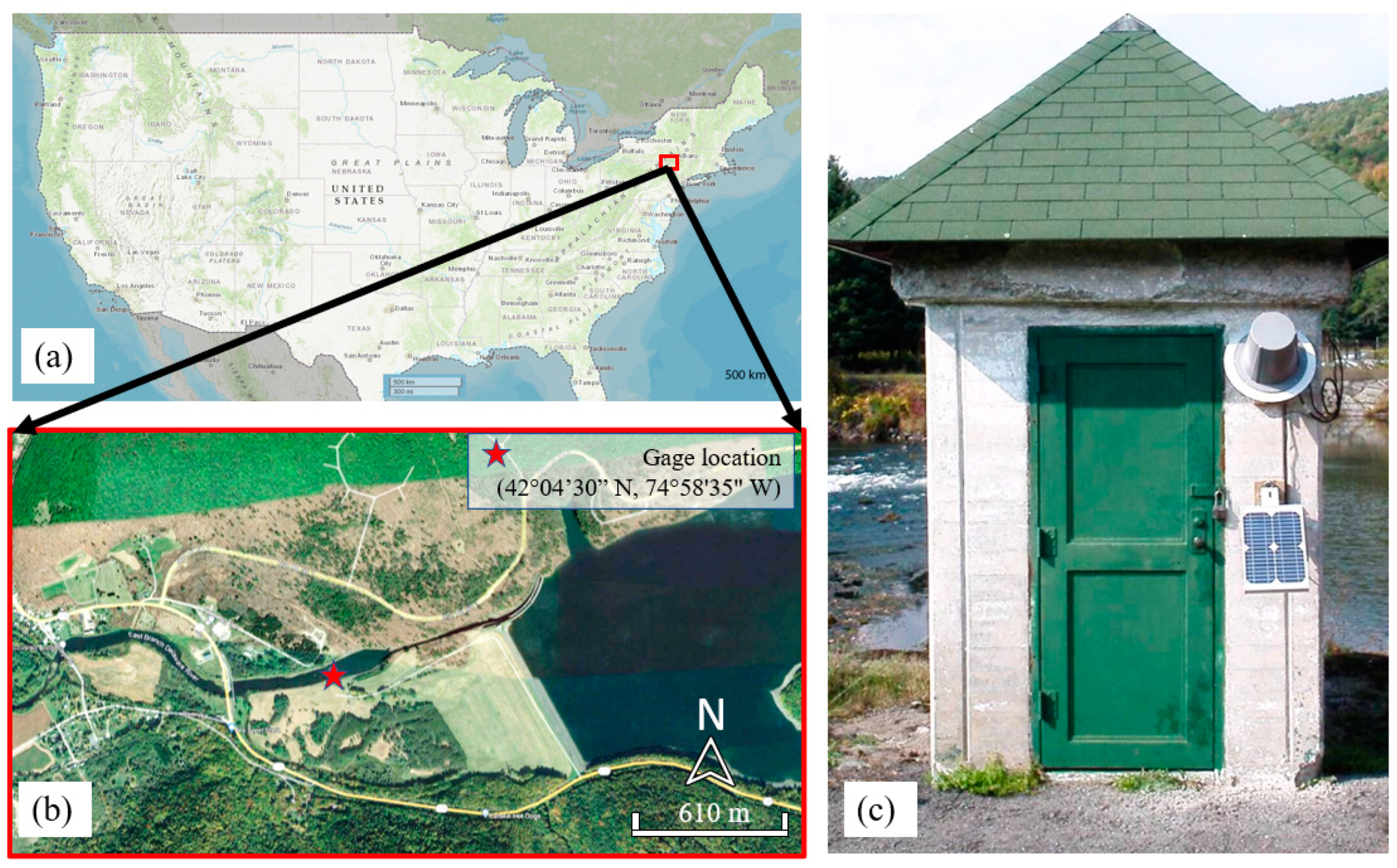
2.1. Study Location and Data Source

The river flow measuring site considered in this study is situated along the East Branch Delaware River in Delaware County, NY (Figure 1). The latitude and longitude of the study site are 42°04′30″ N, 74°58′35″ W with the coordinate system “North American Datum of 1983”. The identification number of the hydrologic unit in the USGS Water database of it is 02040102, on the left bank half miles downstream from Downsville Dam, at the downstream end of the outlet channel of Pepacton Reservoir, and one mile east of Downsville. The contributing drainage area of the measuring point is 372 mi2. The river flow recording gauge datum is 1101 ft. The study location is the situation at the hamlet, Downsville, a census-designated place which was a village in Colchester town, Delaware County, NY.
The period of discharge record is from July 1941 to the present. Range of the discharge time series considered in this research is 1 July 1941 to 31 December 2021, with 29,393 observations. The maximum yearly flow recorded within the entire period after the construction of Pepacton reservoir was 17,700 ft³/s on 18 September 1946 with a water level of 12.08 ft and a minimum flow of 0.6 ft³/s on 11 October 1991 with the minimum water height, 1.39 ft on 17 January 1964. The extreme water level recorded outside the period of record was 16 ft on 9 October 1903 during a flooding event in the surrounding area. Extreme river flow recorded outside the period of record before the construction of the Pepacton reservoir was 23,900 ft³/s on 26 November 1950 with a water level of 14.52 ft [USGS 2022].

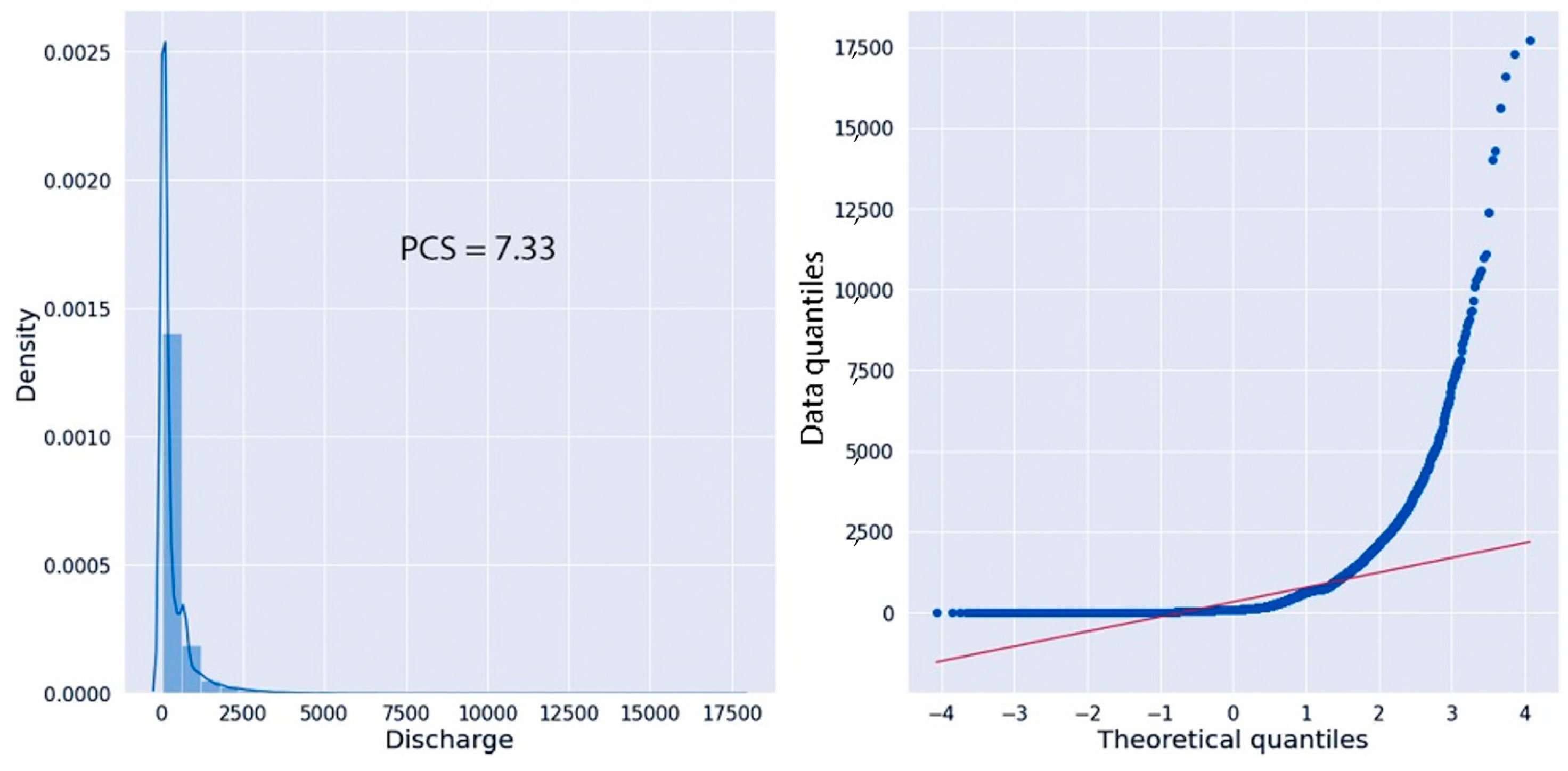
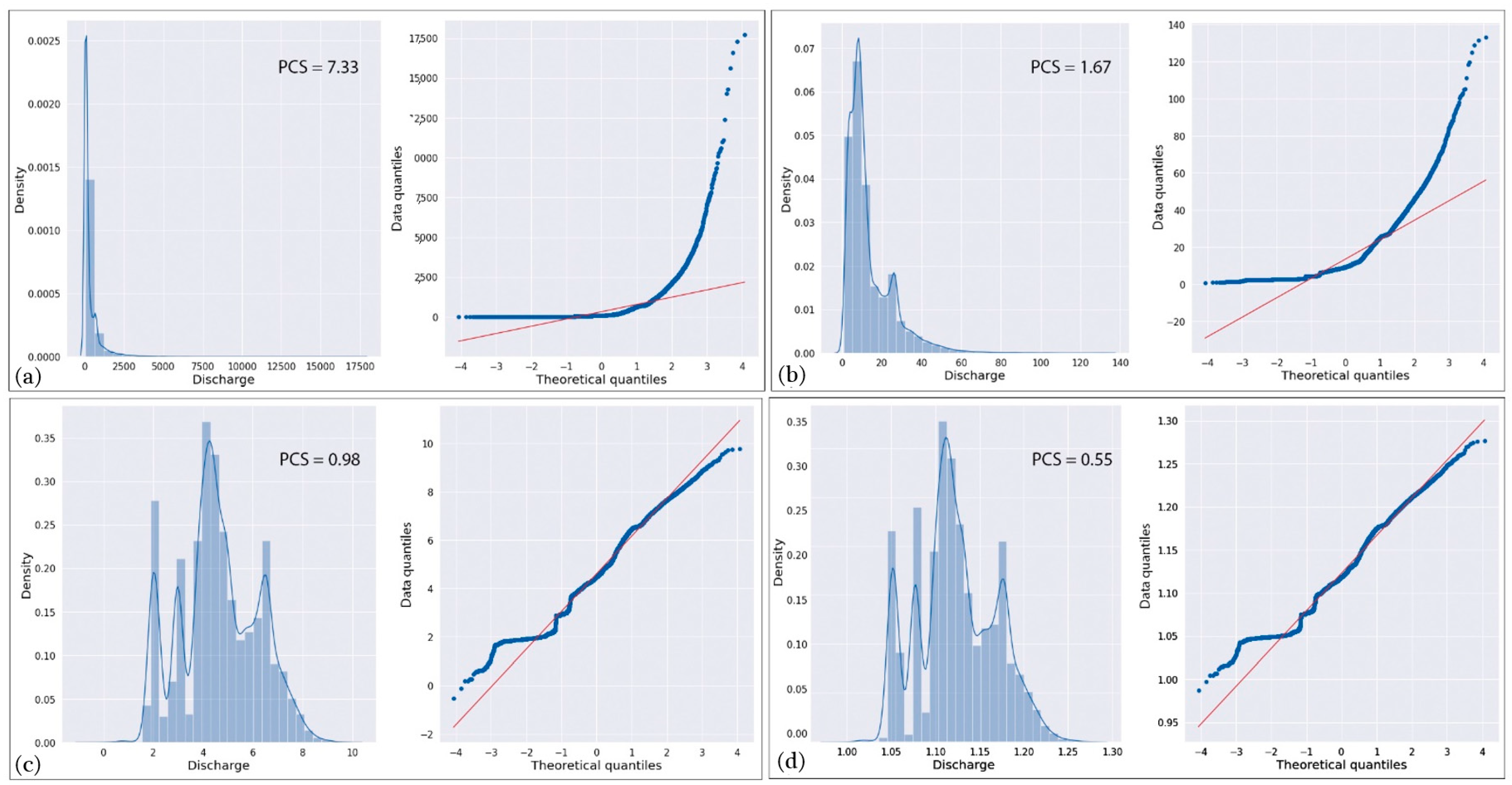
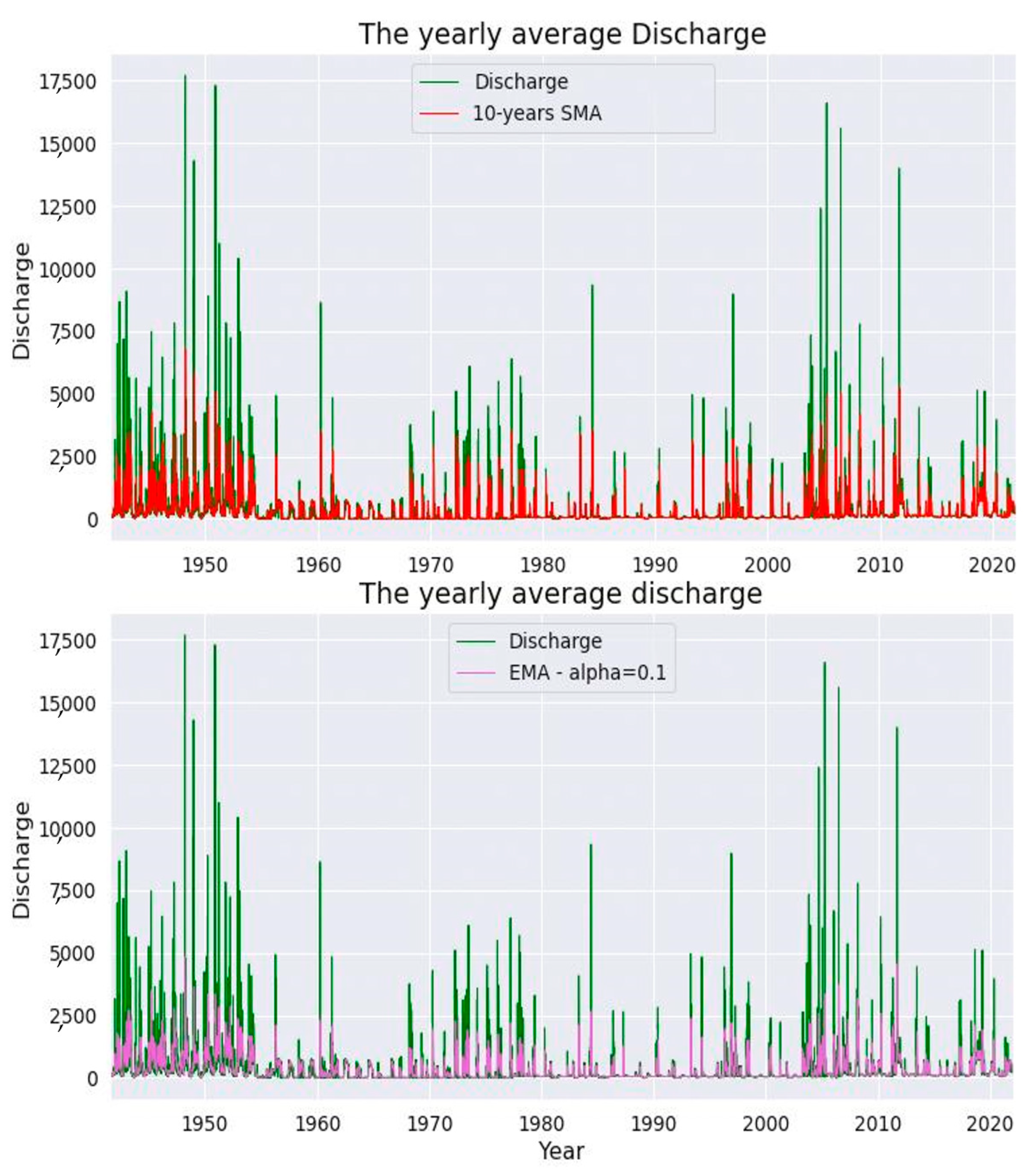
2.2. Univariate Exploratory Data Analysis and Feature Engineering

To obtain the characteristics and attributes of the dataset with discharge series, EDA is performed. EDA is a process where the internal distribution of a dataset is extracted through various graphical visualization and summarizing techniques. EDA involves a critical process of conducting an initial exploration of the variables to investigate the anomalies and hidden patterns. It is the first step toward data preprocessing for ML/DL algorithms. In this study, steps in EDA can be further categorized into two parts. It involves descriptive statistics, outlier detection, and probability distribution to determine the skewness. As the scope of this research is univariate analysis, i.e., only one variable (discharge) (Figure 2), a brief study is performed in the descriptive statistics (Table 1). They are counting the number of observations, obtaining the central values (e.g., mean, median, mode), spread (e.g., standard deviation), range (e.g., minimum, maximum), percentile distribution, interquartile range, and quantifying missing data. In probability distribution, a graphical representation using a histogram and the coefficient of skewness is used to analyze the normality of the discharge series. In this study, the discharge series consists of a significant number of extreme values/outliers. Storm events with a significant amount of rainfall have the greatest impact on the high values of discharge volume. Detecting the outliers revealed both extreme events and erroneous measurements of discharge.
Univariate outlier detection for the discharge series is performed using the inter-quantile-range (IQR) rule. According to the IQR proximity rule, a value of the continuous numeric variable is considered an outlier if it stays outside the upper boundary, i.e., 75th quantile + (IQR × 1.5) or lower boundary, i.e., 25th quantile- (IQR × 1.5) where the IQR is expressed by the difference between 75th quantile and 25th quantile.
After the EDA step, FE is performed. FE is the most crucial step to obtaining the appropriate dataset for training/testing the LSTM algorithm. In FE, imputation is to make the data set consistent, normality check, necessary data transformation if applicable, and data standardization is performed. Without a successful FE, any data-driven method may not yield a satisfactory performance with minimum error. An adequate optimization through the iterative gradient descent cannot be reached without successful scrutiny of the dataset. Therefore, a comprehensive FE is performed to transform the dataset most suitable for the learning algorithm of LSTM. As the discharge variable has some null values, imputation with the median of the series is performed to make the series consistent. Direct discarding of the observations with null values can also be considered. However, this technique is not recommended as it reduces the shape of the dataset by reducing the observed data point.
After the imputation task, the normality of the discharge series is checked using a visualization technique accompanied by the coefficient of normality measure, e.g., Pearson Coefficient of Skewness (PCR). Normal distribution is the most crucial factor in the field of data-driven predictive analysis, e.g., deep neural network regression. Smooth progress towards minima in gradient descent is required to reach the objective function that the step sizes be updated at the same rate for the values of each feature used in the analysis, which can be achieved by increasing the normality of the variable. The logarithmic transformation of the discharge series conveyed a significant increase in normality. In addition, processing and recalling long-term information in time series data is a unique feature of the LSTM model, which makes it different from the traditional feedforward neural network. Therefore, a combination of appropriate feature engineering to increase the normality with the robustness of the LSTM algorithm is applied in this study to obtain satisfactory performance in discharge prediction. As the distribution of the values of river discharge series is highly skewed to the left, indicating non-normally distributed data, the traditional ML and neural network regression algorithms, without appropriate data transformation, do not offer satisfactory performance even with good optimization. Therefore, the LSTM, which is a special type of RNN, is used to forecast the river discharge values in this study. In the next section, a detailed explanation of how the LSTM is utilized for the river discharge time series is presented.
As the distribution of the discharge series is found to be highly skewed, data transformation is performed to decrease the non-normality of the series. In this study, three methods of data transformation are considered, e.g., logarithmic, square-root, and cubic transformation, to transform the distribution of the features more to the normal distribution. Pearson’s coefficient is used as a numerical indicator of normality. In Figure 3 multiple data transformation techniques are applied to observe the shift in the skewness i.e., in-crease/decrease in the normality. Logarithmic transformation outperforms other transformation functions, distributions of the transformed and observed discharge series can be seen. Data transformation with all three functions mentioned above helps to increase the normality, thus decreasing the skewness. Pearson’s Coefficient of Skewness (PCS) is also added to the individual figures to obtain an idea of the degree of the skewness. Logarithmic transformation with the lowest PCS of 0.55 outperforms other transformation functions. It reduced the right-skewness more than other functions, which can be observed in Figure 3. As the PCS value from the logarithmic transformation is promising compared to all others, the data series from this transformation is considered in this research. Logarithmic transformation outperforms other transformation functions, e.g., it reduced the non-normality significantly by changing the value of Pearson’s coefficient of skewness (PCS).
The autoregressive integrated MA model is the most extensively used parametric time series method. Although determining trend significance can be challenging, among the analyses and different methods, the most direct approach for detecting discharge trends in a time series is the MA method. The MA method, as one of the most fundamental ways for analyzing meteorological and hydrological data, smooths and clarifies trend lines by screening out frequent random variations in hydrological data. The focus of the analysis is more on the accentuating longer-term patterns rather than short-term fluctuation for a better representation of MA. It can be calculated for a different duration and number of years by shifting the average value of specified variable year by year and including all the data points, and concluding the entire data set at the end of the process for the target duration range. For this study, the MA method was used to analyze discharge variation as a yearly average for the duration of 81 years (from 1941 to 2021). The average discharge was investigated by considering two types of MA models: the Simple Moving Average (SMA) and the Exponential Moving Average (EMA). SMA is an accounting MA that is calculated by averaging recent discharges and adding recent values. Then dividing, the outcome by the number of periods in the data range (Equation (1)).
S M A = Q 1 + Q 3 + Q 3 + + Q N N
where N is the total number of periods, and Q N is the discharge value at period N.
An exponential moving average (EMA) is a type of MA that assigns a higher weight to the recent data and measures the direction of the discharge trend over a period of time (Equation (2)). The EMA benefits from the recent discharge changes and is capable of capturing the possible recent year trend and climate change impact.
E M A = Q t × k + E M A t 1 × ( 1 k )
k = 2 ( N + 1 )
where k is the weighted multiplier, t is represented as the present values, and ( t 1 ) is a symbol for the previous period. The time interval is dependent on the time-series dataset and the interval in the actual dataset (i.e., day, hour, or minute).
Both 10-year SMA, EMA, and MA analysis results in the Figure 4 illustrated the average discharge to be highest in 1945 before decreasing to the minimum in late 1955. However, the minimum range of average discharge continued for over a decade, compared to the second rise in its values in 1975, which was still about half of the maximum discharge average experienced in 1945. The decadal decrease was defined for more than two decades after 1975, along with the same increasing trend and more variance until 2012.
Through the data standardization process, the values of a variable are rescaled so that the variable has a mean 0 and variance of 1 (or Z-score normalization), which is identical to the bell-shaped normal distribution curve. As the variable considered in this study is the continuous independent variable, the standardization of the variable is crucial for training/testing the neural network algorithm. Standardization is an important step for the optimization problem. The LSTM RNN model uses the gradient descent technique, where the feature value (discharge) affects the step size of the technique. Smooth progress towards minima in gradient descent requires the update of the steps at the same rate for all the feature values. A standardized variable is a prerequisite for reaching the minima in the gradient descends process.
X n o r m = X X m i n X m a x X m i n
All the values in the discharge series are normalized to prepare the training dataset for the LSTM model.
Equation (4) shows the formula for the normalization of the discharge series. The difference between the discharge value and the minimum of the entire discharge series is divided by the range of the series and provides the standardized data, which is further used in the training/testing process of the LSTM. The entire standardized discharge series is split into two portions, i.e., a training set that is used to train the model and a testing set that is used to test/evaluate the model. Seventy (70) percent of the dataset is used for training, and thirty (30) percent is used for testing. In a nutshell, EDA and FE are pivotal steps for the satisfactory performance of the predictive model.

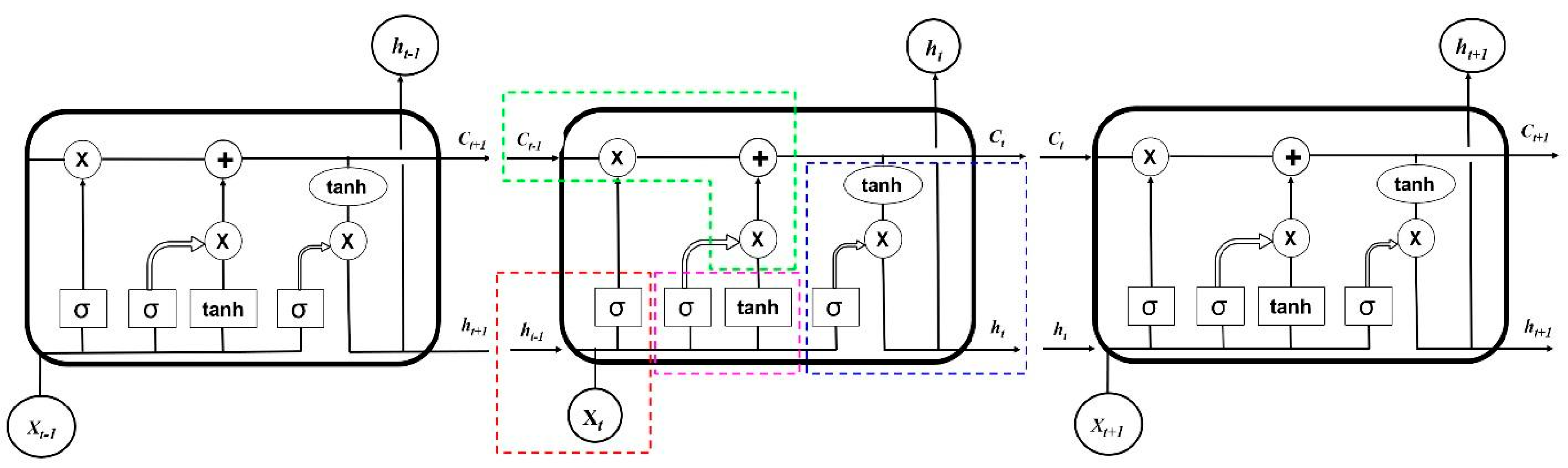
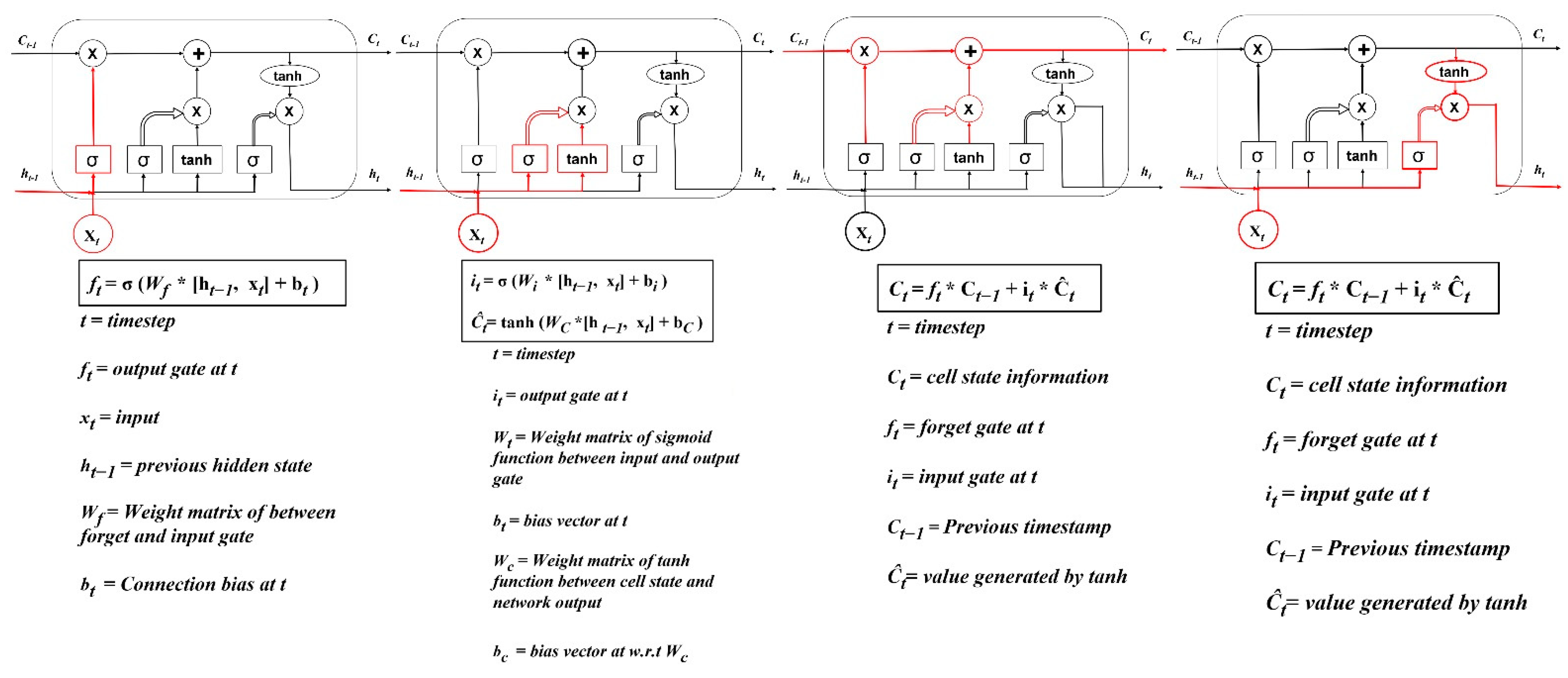
2.3. Long Short-Term Memory (LSTM) Recurrent Neural

LSTM is a special type of RNN which is frequently applied specially in sequential forecasting. LSTM feedback connections are the principal component of processing and recalling long-term information and a unique feature that makes it different from the traditional feedforward neural network. This unique property of LSTM is utilized in processing the sequence of datasets, e.g., discharge time series, and treating all the data points independently. LSTM RNN is suitable for various water-related variables with time series, e.g., river flow, groundwater table, precipitation, etc. [61,66,67,68,69,70].
Both long-term memory (c[t − 1]) and short-term memory (h[t − 1]) are processed in a typical LSTM algorithm through the utilization of multiple gates to filter the information shown in the Figure 5. For an unchanged flow of gradients, forget and update gates update the memory cell state [71,72]. Three gates, i.e., input gate ig, forgot gate fg, and output gate og handle the information flow by writing, deleting, and reading, respectively. Hence, LSTM is capable of memorizing information at different time tags and intervals, making it suitable for time series prediction within a certain interval [73]. In the forget gate, long-term information enters and passes through a filtration where unnecessary information is discarded. The forget gate filters out unnecessary data by using the sigmoid activation function where the range of the function is 0 (gate closed) and 1 (gate open). Input gate filter and quantify the significance of new data coming as input to the cell. Such as the forget fate, the input gate filters out information by using binary activation functions and controls the flow of both long-term and short-term information. The output gates regulate the value of the upcoming hidden state, which is a function of the information on previous inputs. The entire schematic of the information flow through LSTM cells and related equations for each cell can be seen in the Figure 6 and Table 2, respectively.
In the above equations h t represents a vector for the hidden state, which is linked to the short-term memory. The C t is the cell state linked to long-term memory, and C ˜ t is the candidate for cell state at time tag t, which is used to filter important data to store over time. Several weight matrices are used in the input gate, forget gate, output gate, and cell state. They are indicated as W i , W f , W o , W c . For current input X t , several weight matrices and biases, i.e., V i , V f , V o , V o , and b i , b f , b o , b c are used. The operator ⊙ denotes the Hadamard product (element-wise product)
Hyperparameters are required to be tuned to maximize the performance of every ML model. Other parameters involved in the stochastic process of any ML model are learned through iteration. However, the hyperparameters are decided manually. Therefore, they must be tuned in to achieve satisfactory performance. As there is no systematic approach to selecting the hyperparameters, the iterative trial and error method is applied to find the most appropriate values where the model performs best. In this study, Keras, a python library that offers a space search for ML algorithms, is used to find the best combination of the hyperparameters. Hyperparameters of the LSTM algorithm considered in this study are the size of epoch and batch and number of neurons [74,75].

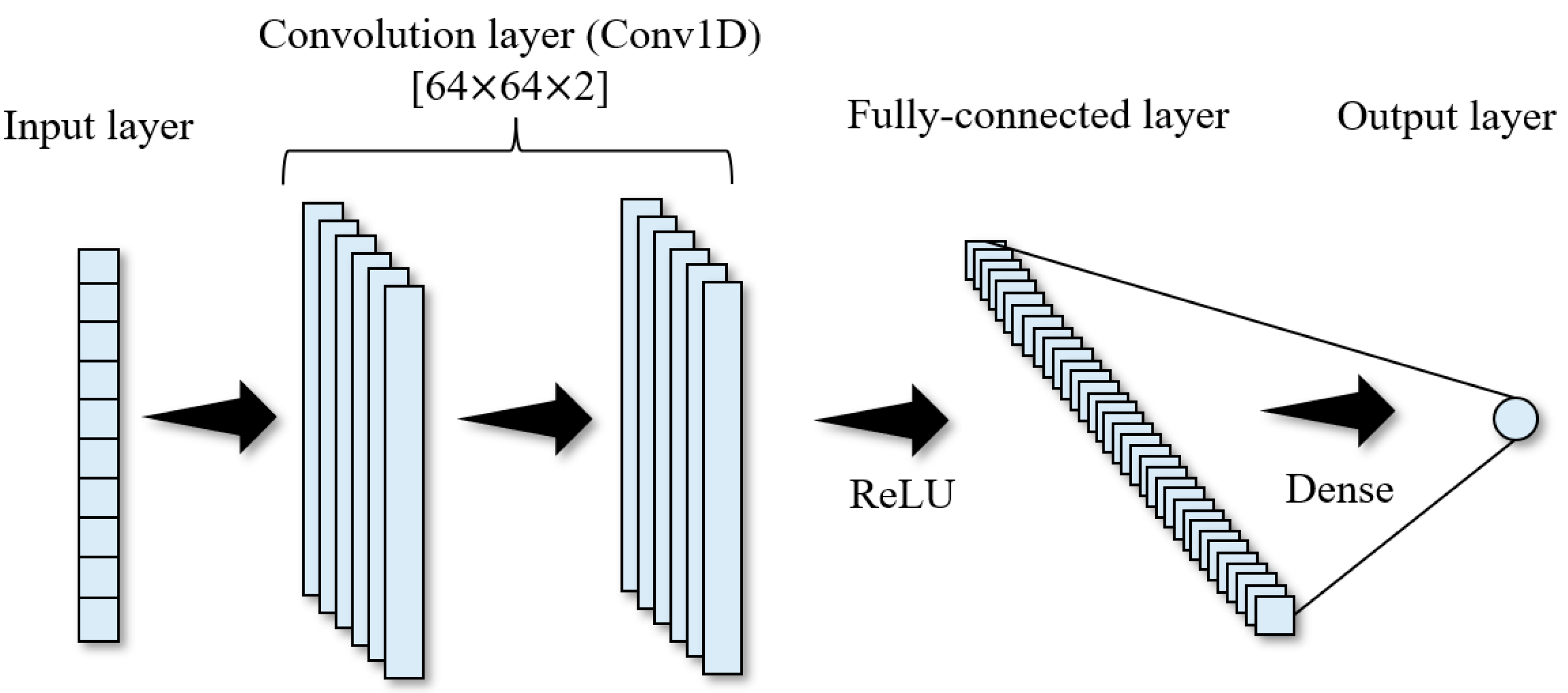
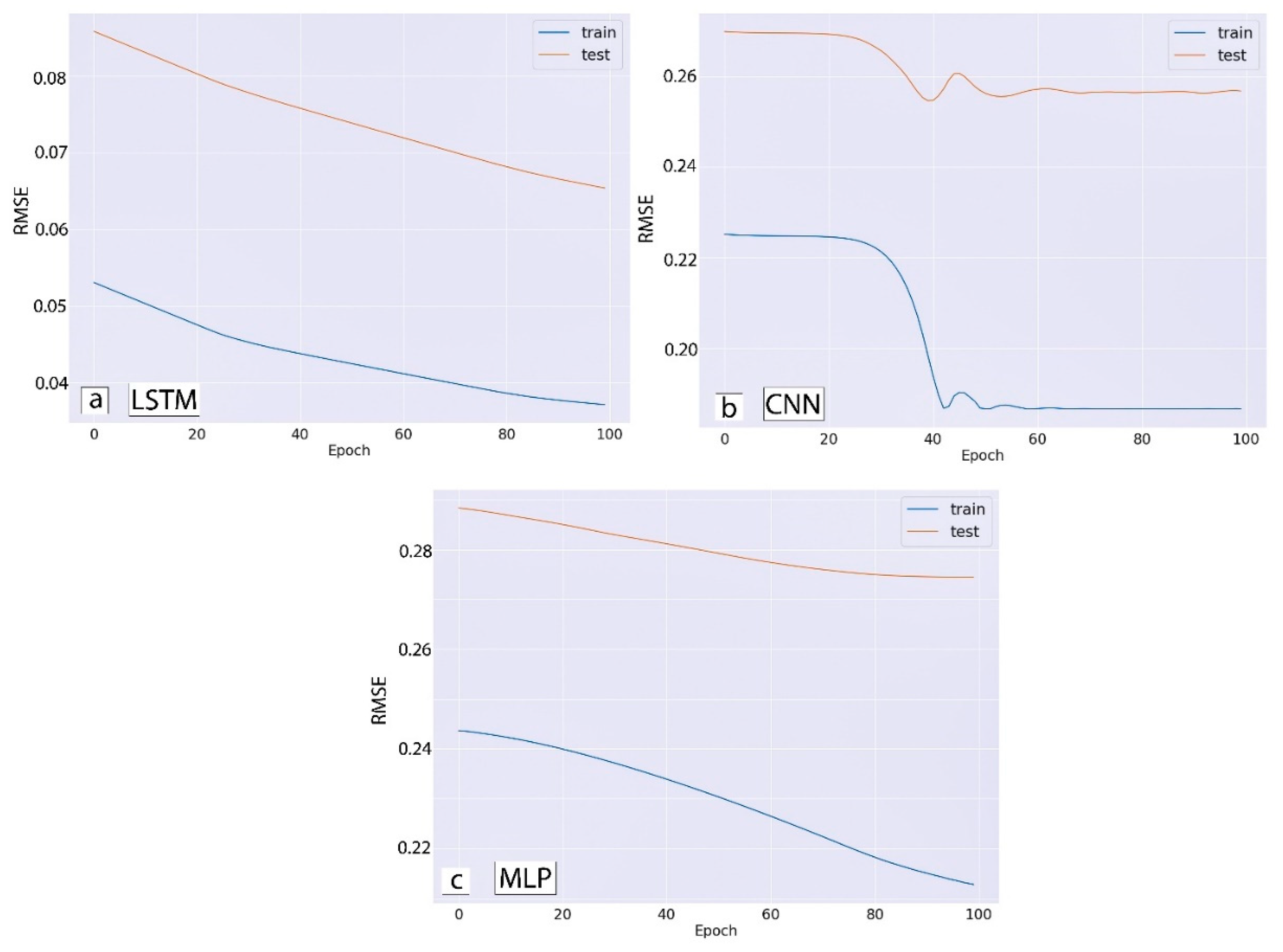
2.4. Comparative Study

A comparative study is performed to investigate the performance of the LSTM algorithm with other DNN time series prediction algorithms. In this study, Multilayer Perceptron (MLP), RNN, and Convolution Neural Network (CNN) are used to predict the discharge. A multilayer perceptron (MLP) is a fully connected type of feed-forward neural network (FFNN). An MLP is constructed with three layers, i.e., an input, hidden, and output layer. Except for the nodes in the input layer where the inputs are embedded, each node in the hidden layer is a neuron uses a nonlinear activation function. MLP is based on supervised learning and backpropagation techniques for training. All the layers and non-linear activations distinguish the MLP algorithm from a linear perceptron-based prediction. Convolutional neural network (CNN) is a special type of neural network mathematical convolution. In general, matrix multiplication is at least one layer. CNN is specifically designed to preprocess the pixel data applied in image processing. CNN substitutes the mathematical operation known as convolution for generic matrix multiplication in at least one of its layers. A convolutional neural network is built of an input layer, hidden layer(s), and an output layer to generate the outcome of the model. Unlike the feed-forward neural network, the hidden layers of CNN include layers to perform convolutions on the input data. Convolutional layers are among the hidden layers in CNN. This typically contains a layer that does a dot product of the input matrix of the layer with the convolution kernel. The convolution procedure develops a feature map as the convolution kernel moves across the input matrix for the layer, adding to the input of the following layer. Following this are further layers such as normalizing, pooling, and fully connected layers. In this study, a sequential model of 1D convolutional neural network (Conv1D) with a fully connected network is used to predict discharge time series. A total of 64 filters and 2 kernel sizes have been considered for Conv1D. The activation function was ‘ReLU’ for both the Conv1D and fully connected layer. A 1D Max Pooling was added with a pool size of 2. A total of 50 neurons with two hidden layers have been used for the fully connected network (Figure 7).

2.5. Error Analysis

The literature provides a wide range of evaluation matrices that have been mostly used in hydrologic modeling to compare the prediction’s accuracy. The predictions’ error defined via various methods represents the difference between data points as the observed real values and predicted values as the measured ones. Multiple model variability settings were used in this study. The top four standard performance assessment methods to evaluate the analytical output and draw conclusions were Root Mean Square Error (RMSE), correlation coefficient (r), relative error (RE), and the Nash Sutcliffe model efficiency coefficient (E). Multiple performance indicators should indeed be employed to assess model accuracy rather than one which can also effectively capture the high streamflow time series values. The term “norms” refers to the varied forms of multi-dimensional error measures. The norm normalizations lead to a relative dimensionless metric and reduce the error measures’ sensitivity to the dimensions of the data frame. The most popular evaluation metric is the Root Mean Square Error (RMSE), as the function is more sensitive to significant errors. That’s because the squared term multiplies greater errors exponentially more than smaller ones. RMSE is the mean of the absolute value of the errors and is normalized by the number of data points, N:
R M S E = 1 N t = 1 N | Q t ( o b s ) Q t ( c o m ) | 2
where Q t ( o b s ) = observed discharge, Q t ( c o m ) = computed discharge, so ( Q t ( o b s ) Q t ( c o m ) ) represents the error term between the real and measured value for each data point which is normalized by dividing by the total number of observations after the summation of all terms. The lowest RMSE score corresponds to the best predictive accuracy.
The coefficient of determination ( R 2 ) is a popular performance indicator for the accuracy of the model and the model's fitness to the data points’ values depicted by this metric. The better the model fits the data, the higher the R2 is. The coefficient of determination which is the second error function implemented in this study is represented in Equation (6).
R 2 = ( t = 1 N ( Q t ( c o m ) Q ¯ ( c o m ) ) ( Q t ( o b s ) Q ¯ ( o b s ) ) ) 2 ( t = 1 N ( Q t ( c o m ) Q ¯ ( c o m ) ) 2 ) ( t = 1 N ( Q t ( o b s ) Q ¯ ( o b s ) ) 2 )
where Q ¯ ( o b s ) = average of observed discharge. The R2 range is 0 to 1, with 0 indicating no correlation and 1 signifying perfect correlation between observed and computed values.
M A P E = 100 % n t = 1 n | A t F t A t |
The above equation shows the third performance indicator, the Mean Absolute Percentage Error (MAPE) used in this study. MAPE is a measure of the prediction accuracy of a time series forecasting method. The fourth evaluation metric refers to the Nash Sutcliffe model efficiency coefficient (E) and is one of the most widely used metrics for evaluating a hydrologic model’s performance. E can be classified as one of the scaled forecasts that compare the predicted error to the observed error.
E = 1 t = 1 T ( Q t ( o b s ) Q t ( c o m ) ) 2 t = 1 T ( Q t ( o b s ) Q ¯ t ( o b s ) ) 2
where Q ¯ t ( o b s ) = average of observed discharge, and E is dimensionless with a range of E 1 , with 1 as the largest value that E can obtain, representing the best model accuracy. Having a positive value for E (greater than zero) shows that the prediction and computed discharge value are better than simply selecting the average observed value.

3. Results

LSTM RNN are used to predict the time series of discharge data based on multiple lead times. Several lead time durations, e.g., 1 day, 2 days, 3 days, 4 days, 5 days, 6 days, and 7 days are used to forecast the future values of discharge. Only one lag time, 30 days, is used for the entire analysis to be consistent with the comparison of the model performance. Model performances are recorded for the lead times based on several error indicators to show the efficiency of the LSTM model in predicting the discharge values. Predicted values are compared to the observed dataset, and their difference of them is computed to quantify the performance indicators. Root mean square error (RMSE), correlation coefficient (R-squared), and Nash Sutcliffe (E) error are used to estimate error from the predicted discharge data in the comparative study of LSTM, CNN, and MLP-based predictions. Model performance is improved by the increase in iteration, i.e., an increase in the number of epochs. Performance indicators are obtained through multiple models runs to demonstrate the linkage between the model performance and the lead times in the LSTM model. Hyperparameters of the LSTM model are adjusted to optimize the model performance considering a set of batch size, epoch size, and the total number of neurons.

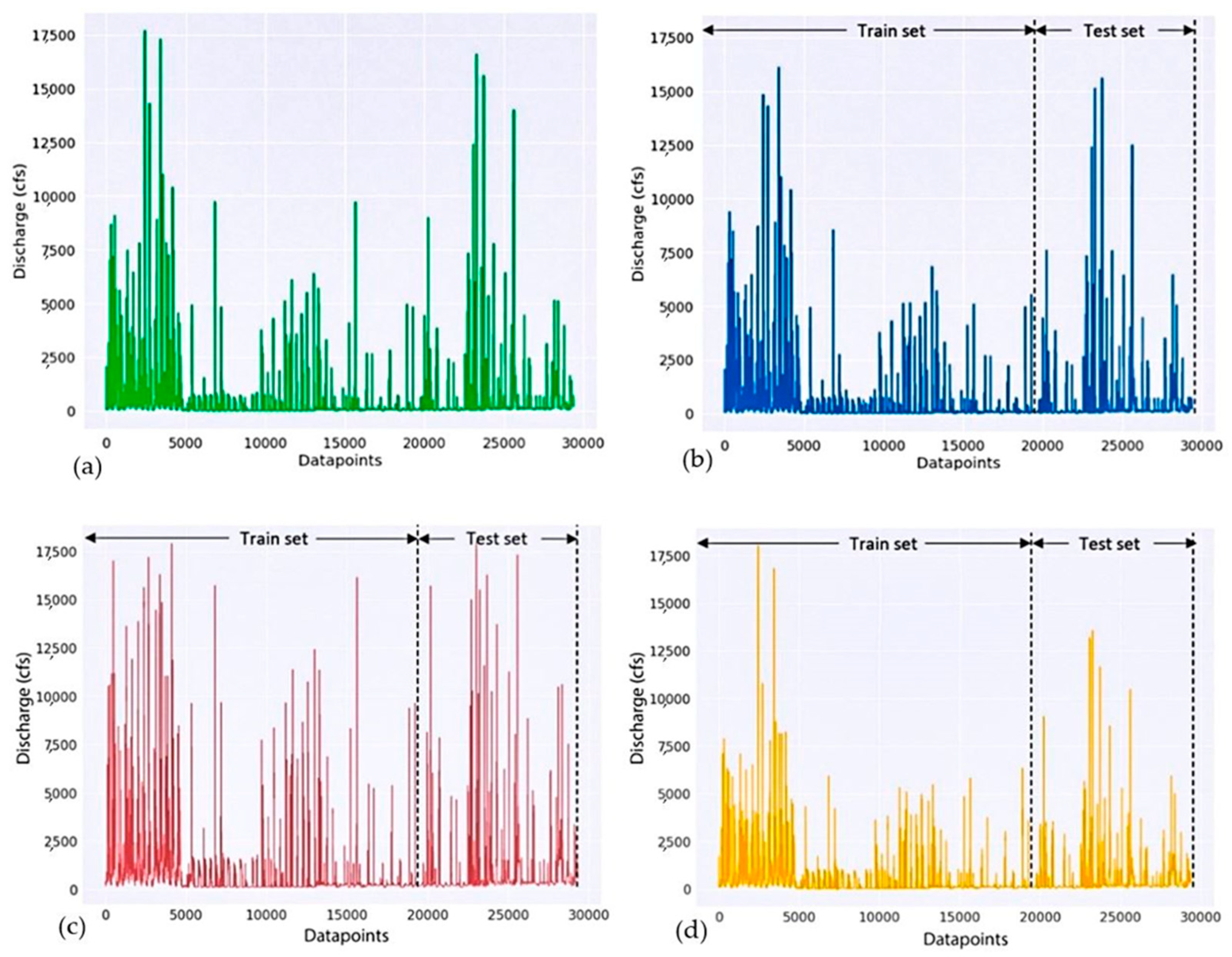
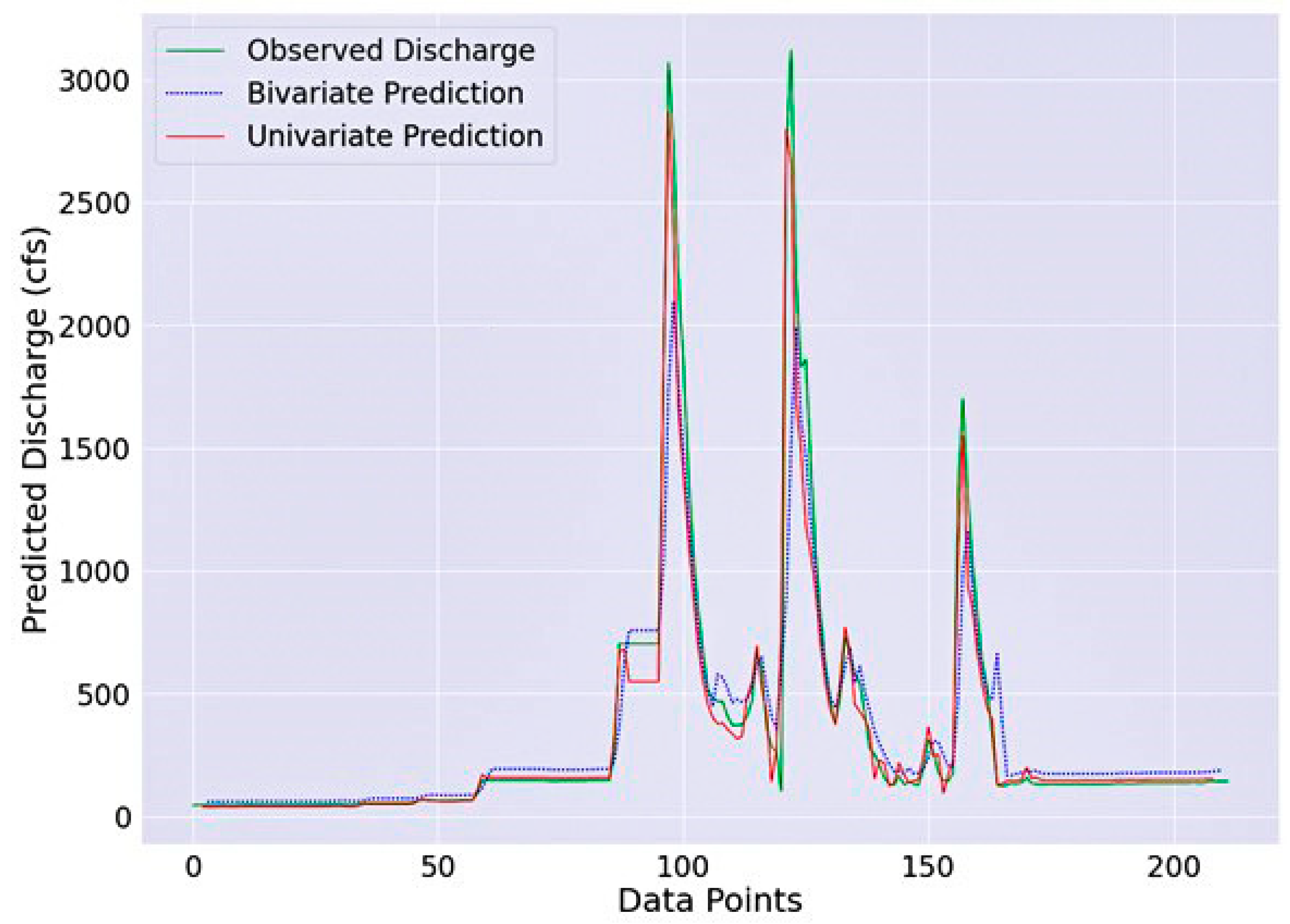
3.1. Predicted and Observed Discharge Series

The output from the LSTM algorithm is compared to the observed discharge data from the USGS database through visualization. A comparative study with predictions from CNN and MLP is also presented to investigate the LSTM performance. Both the observed and predicted discharge time series are plotted in cubic feet per second (cfs) against the number of observations. The overall distribution of the predicted discharge values from LSTM, CNN, and MLP, are approximately identical to the observed data providing a satisfactory performance of all the algorithms. However, the LSTM approach outperforms the CNN and MLP-based approaches in predicting discharge based on past values. The performance indicator, RMSE, for the LSTM algorithm is 151.52 ft3/s, where 235.74 ft3/s and 489.07 ft3/s for CNN and MLP, respectively, where the MAPE values are 0.92%, 2.17%, and 2.95%. Model performance improvement through continuous iterations, i.e., with the increase in the number of epochs, is presented in the Figure 8 for all algorithms. However, LSTM ended up with the best performance after 100 epochs among all other algorithms with minimum error. After the LSTM model is trained with the training portion of the dataset, the entire observed dataset is fed to predict the outcome and divided into training and testing sets with the proportion of 70% and 30%. The training dataset is used to train the model, and the testing dataset is used to evaluate the model’s performance. Observed data are shown in a with green color, and the training portion of the dataset is illustrated in sections (b–d) for LSTM, CNN, and MLP, respectively. The RMSE values of the training and testing portion are 0.097 and 0.045, respectively. The lowest RMSE score corresponds to the best predictive accuracy and shows the better satisfactory performance of the LSTM algorithm.
It is common practice to utilize measured or predicted precipitation data files in any approach for estimating future river flows during a flood event since the magnitude of the precipitation event is the most significant factor affecting the magnitude of the flood event. In addition, we considered precipitation data from the closest station because it is one of the most important contributing factors in the dynamics of river discharge. We took into consideration a dataset with a range of a year (2017) because both the discharge and precipitation data were readily available. Univariate prediction for future discharge scenarios based on past values can be highly efficient in reaching a quick and effective decision for water resource managers and engineers. It is fairly simple to see the future situation of the river flow at a point location (e.g., after 1, 3, or 7 days) based only on the past recorded discharge values. The 30 days duration is used for the time lag so that the past recorded discharge values considered for each lead time can be consistent. We also explored the bivariate (precipitation and discharge) prediction comparing them with the observed discharge values (with the lead time of 1 days) for the year 2017 and univariate prediction. Both approaches showed satisfactory performance with the RMSE score of 151.52 ft3/s and 389.77 ft3/s, respectively, for univariate and bivariate (Figure 9). The RMSE for 2 days and days lead time resulted in 1.98 and 4.17, respectively. Bivariate prediction conveyed a slightly lower score compared to univariate prediction, where only previous discharge values were used. Increasing the lead time from 1 day to 2 days or 3 days enhances the error and reduce the accuracy as expected. This may have occurred as a result of the predictive analysis for a point location with no spatial variability. In order to obtain a more robust prediction with more influencing factors, additional exploratory analyses and feature engineering need to be performed to understand the internal dynamics of the input variables at a point location, however, for effective decision-making, multiple observational stations for both the input variable (e.g., precipitation) and output variable (e.g., discharge) to reach a better prediction incorporating both spatial and temporal dynamics in the prediction.
The availability of reasonably accurate quantitative rainfall forecasts allows flood predictions to be made in advance of the occurrence of severe rain events using physically based modeling. It is to be expected that the predicted flowrates from the LSTM algorithm would not similarly predict high flowrates in subsequent days on the day before the rain event occurred. However, in practice, the LSTM predictions in some cases, but not in all, correctly predicted daily flow peaks in days to come on the day before a large rain event would occur. For example, on 5 June 2017, the observed flowrate was 175 ft3/s. The predicted flowrates for June 6, 7, and 8th were 1065, 1227, and 1186 ft3/s, correctly identifying a large flood event caused by rain on June 6th. However, this pattern of anticipation of flood peaks was not always present. On May 1, 2017, with a daily flowrate of 103 ft3/s, the predicted flowrates for May 2, 3rd, and 4th were 311, 238, and 320 ft3/s; the observed flowrates were 2700, 3120, and 2190 ft3/s. Further investigation is needed to seek an explanation for the erratic prediction of future flood events by LSTM on the day before large rain events.
Performance indicators are documented for several lead times and illustrated in the Figure 10. Lead times are pivotal parameters of the LSTM algorithm toward model performance. Lead times values considered in this research are from 1–7 days. The values of RMSE increase with the increase in the number of lead times, whereas of R 2 and E decreases showing the poorer performance in the model performance in the Figure 10. Lead time is the length of a cutout of a time series that is used to predict the output (recession rate) at a future time step. The increase in the time leads to convey increase in the duration of prediction, e.g., discharge prediction after 2 days from the present. The R2 value of 0.093 for the lead time of one day is the lowest among all the lead times.

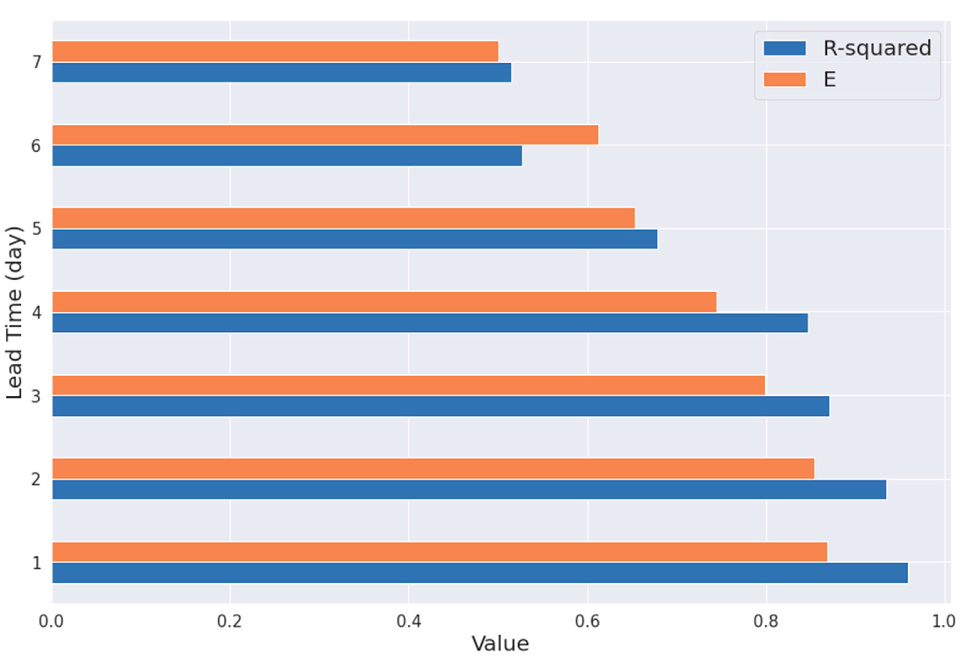
3.2. Model Evaluation Matrices and Improvement

The performance of the LSTM neural network is evaluated using three performance indicators, e.g., the coefficient of determination ( R 2 ), Root Mean Square Error (RMSE), and Nash Sutcliffe model efficiency coefficient (E). The performance variation with the change in the lead time is represented in the Figure 10. Further, the performance of the model was also evaluated and improved by increasing the number of iterations, i.e., an epoch in the neural network. The value of RMSE is observed with the increase in the number of iterations/epochs in the LSTM neural network in the Figure 11. The number of epochs is increased up to 100 to increase the performance and converge to a more stable narrow range of RMSE values. The RMSE of the normalized values is found to decrease from 0.09 to 0.037, which indicates satisfactory performance in the LSTM algorithm. The model performance increases significantly from the very beginning of the iteration for both the train and test scenarios. Changes in the RMSE values are obtained for both the train and test datasets marked in blue and orange color. A comparatively mild decrease in the RMSE value, i.e., an increase in the model performance, can be observed between 20 and 100 epochs. Several local abrupt variations in the performance can also be identified after approximately 5 epochs. The trend of change in the decrease in the RMSE of the normalized values for the models shows that approximately 100 epochs may yield the best performance.

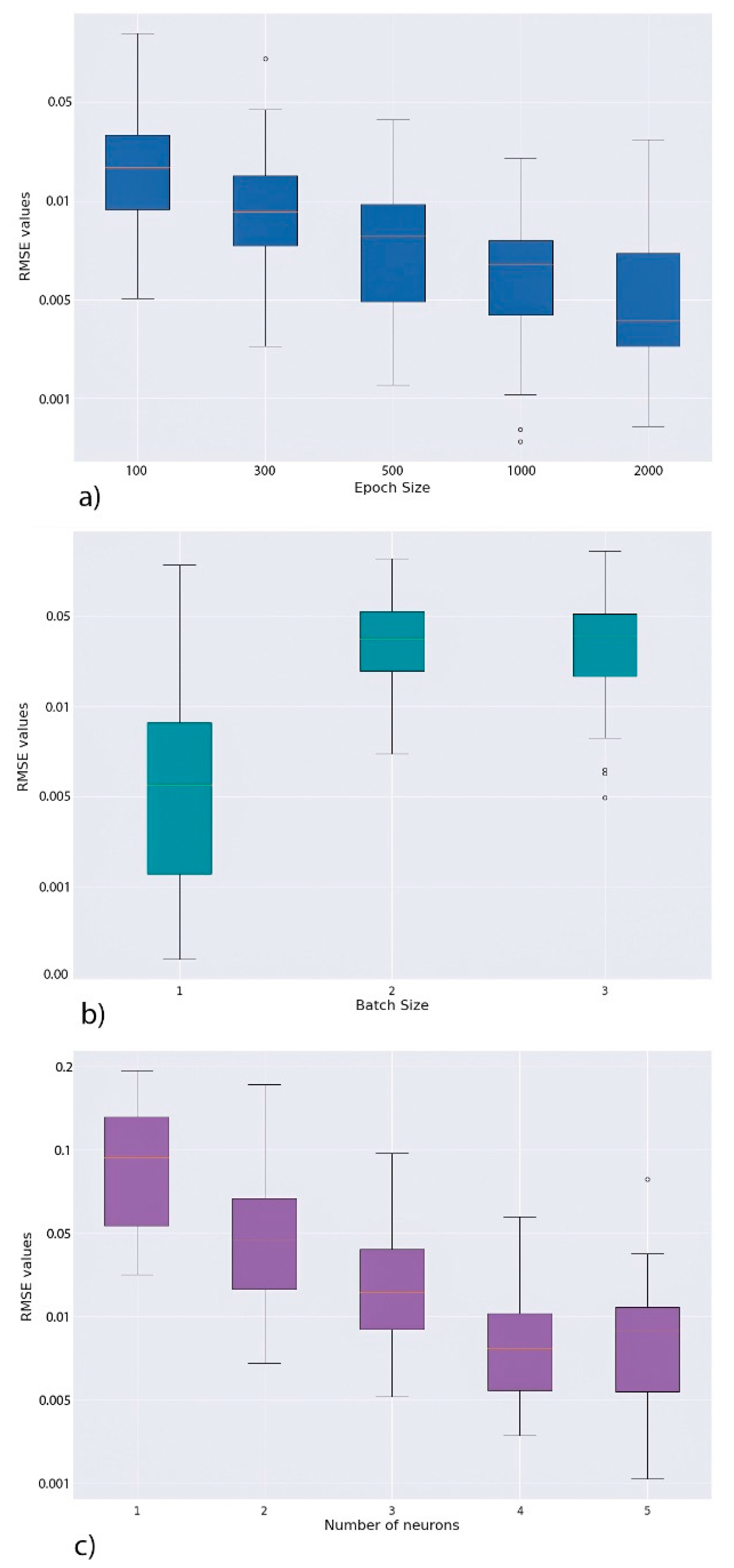
3.3. Hyperparameters

Tuning the hyperparameters of LSTM can be intimidating as there is no simple and robust hypothesis to perform the task of optimizing the model [76]. In order to conduct hyperparameter tuning for LSTM algorithms, a systematic approach should be undertaken to perceive the dynamical and stochastic characteristics of the process [77]. In this study, LSTM neural network is applied discharge time series data. The performance of the model is further improved by tuning the size of epoch and batch and the number of neurons for the neural network stochastic procedure. The tuned parameters are only applicable for the discharge time series used in this study to the stochastic nature of the neural network optimization.
Epoch size is tuned first for constant batch sizes of four and a single neuron. The number of epochs considered to observe the variation in the performance are 100, 300, 500, 1000, and 2000. Similarly, the number of batch sizes of 1, 2, and 4 and neurons of 15 are considered to keep the epoch size constant in 2000 to see the model improvement. An epoch size of 2000 is selected to further the tuning task with the batch size and the number of neurons as it contributes to the lowest RMSE value. A batch size of 1 and 4 neurons provides further lower RMSE values, which can be seen in the Figure 12. Therefore, an epoch size of 2000, batch size of 1, and a number of neurons of 4 are selected as the best hyperparameter combination for the LSTM algorithm to maximize the model performance.

4. Conclusions

Time series prediction for river flow is a pivotal task in the field of water resource management. Discharge is the most important parameter in various aspects of water resource engineering and management, e.g., flood and irrigation warning systems. On the contrary, the application of the data-driven prediction models is highly efficacious in predicting various hydrological variables without taking complicated equations and assumptions into consideration. In this study, river discharge is predicted using the most powerful neural network in predicting sequential data, i.e., LSTM RNN. The LSTM algorithm can recall both the short- and long-term pattern of the time series to forecast. The range of the discharge time series considered in this research is quite large, containing multiple seasonal dynamics and climatic variations. Traditional physics-based numerical modeling tool requires assumptions, other correlated variables, and expensive calibration of the parameters. Compared to the other neural network regression models, LSTM is proven to show good performance, especially the time series prediction. As the river flow provides sequential data which has high temporal dynamics, LSTM is used to quantify future values based on past data. As the shape of the discharge dataset is comparatively large, containing 29,392 observations data points from July 1941 to December 2021, LSTM algorithms showed highly satisfactory performance with longer lead periods.
This study contributes to a reproducible template to investigate the uniqueness of the temporal dynamics of river discharge through extensive EDA. The hidden pattern of the distribution of discharge values through over 80 years of data is discovered in various up-to-date data exploration tools, which is a mandatory requirement for the satisfactory training of the LSTM algorithm. After a successful training step, LSTM is tuned and optimized through an explicit iterative performance record which can further be transferred to forecast discharge value in identical geographical locations. The performance of the LSTM algorithm in predicting the river discharge illustrates the algorithm is highly suitable to the discharge time series. Several performance indicators show promising performance with minimum error compared to the other DNN approaches.
In comparison to a univariate prediction, which relied solely on prior discharge levels, a bivariate prediction resulted in a slightly lower score. The predictive analysis for a point location with little spatial variability may have caused this to occur. Additional exploratory research and feature engineering must be performed in order to fully understand the internal dynamics of the input variables at a given point location in order to obtain more reliable predictions with more influencing factors. However, to make effective decisions, it is necessary to use several observational stations to gather data on the input (such as precipitation) and output (such as discharge) variables. This allows for more accurate predictions that account for both spatial and temporal dynamics. Consequently, in our upcoming research, we are quite eager to track the spatio-temporal dynamics of the contributing factors at the watershed scale. It should also be considered that there are a couple of drawbacks of using LSTM along with the advantages, which are: (1) the time consumption on training the model, which LSTM analysis requires more time and running the model over a large dataset can take longer than other conceptual models. In this study, the computational effort/time required for the LSTM algorithm was found to be considerably high. (2) The low-speed process also resulted in the requirement of using more memory and storage potential of the system, which again can cause a challenge for training on a large dataset, likewise in this research. (3) Complex process of LSTM for time series data has a high potential of facing overfitting challenges and results in inaccurate, extremely low error measures. (4) Although the ability to compare the difference lead time throughout the entire time series dataset is the key point of implementation of LSTM, we were not able to obtain a satisfactory performance for more than a three-day period for this dataset. Any lead times within a three-day period resulted in satisfactory model performance with low error measures. Future research works should be conducted to incorporate high-performance computing and cloud-based operations to obtain the best result. LSTM models with different configurations should also be applied in different geographical and climatic locations to investigate the transferability of the model.

Author Contributions

Conceptualization, M.A.A.M. and M.K.; methodology, M.A.A.M. and M.K.; formal analysis, M.A.A.M., M.K. and M.M.S.Y.; investigation, M.A.A.M.; writing—original draft preparation, M.A.A.M., M.K. and M.M.S.Y.; writing—review and editing, M.A.A.M., M.K. and M.M.S.Y.; visualization, M.A.A.M.; supervision, M.A.A.M., M.K. and H.S.; project administration, M.A.A.M., M.K. and H.S.; funding acquisition, M.K. and H.S. All authors have read and agreed to the published version of the manuscript.

Funding

This research did not receive any specific grant.

Institutional Review Board Statement

Not applicable.

Informed Consent Statement

Not applicable.

Data Availability Statement

Data collected for the study can be made available upon request from the corresponding author.

Acknowledgments

This study was supported by the Computer Science program in the School of Computing and Analytics at Northern Kentucky University.

Conflicts of Interest

The authors declare no conflict of interest.

References

  1. Meis, M.; Benjamín, M.; Rodriguez, D. Forecasting the Daily Variability Discharge in the Fluvial System of the Paraná River: An ODPC Hydrology Application. Hydrol. Sci. J. 2022, 1–8. [Google Scholar] [CrossRef]
  2. Hossain, B.M.T.A.; Ahmed, T.; Aktar, N.; Khan, F.; Islam, A.; Yazdan, M.M.S.; Noor, F.; Rahaman, A. Climate Change Impacts on Water Availability in the Meghna Basin. In Proceedings of the 5th International Conference on Water and Flood Management (ICWFM-2015), Dhaka, Bangladesh, 6–8 March 2015. [Google Scholar]
  3. Kao, I.-F.; Zhou, Y.; Chang, L.-C.; Chang, F.-J. Exploring a Long Short-Term Memory Based Encoder-Decoder Framework for Multi-Step-Ahead Flood Forecasting. J. Hydrol. 2020, 583, 124631. [Google Scholar] [CrossRef]
  4. Song, X.; Liu, Y.; Xue, L.; Wang, J.; Zhang, J.; Wang, J.; Jiang, L.; Cheng, Z. Time-Series Well Performance Prediction Based on Long Short-Term Memory (LSTM) Neural Network Model. J. Pet. Sci. Eng. 2020, 186, 106682. [Google Scholar] [CrossRef]
  5. Le, X.-H.; Ho, H.V.; Lee, G.; Jung, S. Application of Long Short-Term Memory (LSTM) Neural Network for Flood Forecasting. Water 2019, 11, 1387. [Google Scholar] [CrossRef] [Green Version]
  6. Wang, F.; Chen, Y.; Li, Z.; Fang, G.; Li, Y.; Wang, X.; Zhang, X.; Kayumba, P.M. Developing a Long Short-Term Memory (LSTM)-Based Model for Reconstructing Terrestrial Water Storage Variations from 1982 to 2016 in the Tarim River Basin, Northwest China. Remote Sens. 2021, 13, 889. [Google Scholar] [CrossRef]
  7. Ma, B.; Pang, W.; Lou, Y.; Mei, X.; Wang, J.; Gu, J.; Dai, Z. Impacts of River Engineering on Multi-Decadal Water Discharge of the Mega-Changjiang River. Sustainability 2020, 12, 8060. [Google Scholar] [CrossRef]
  8. Bouwer, H. Integrated Water Management: Emerging Issues and Challenges. Agric. Water Manag. 2000, 45, 217–228. [Google Scholar] [CrossRef]
  9. Evans, R.G.; Sadler, E.J. Methods and Technologies to Improve Efficiency of Water Use. Water Resour. Res. 2008, 44. [Google Scholar] [CrossRef]
  10. Sophocleous, M. Groundwater Recharge and Sustainability in the High Plains Aquifer in Kansas, USA. Hydrogeol. J. 2005, 13, 351–365. [Google Scholar] [CrossRef]
  11. Zhang, X.; Meng, Y.; Xia, J.; Wu, B.; She, D. A combined model for river health evaluation based upon the physical, chemical, and biological elements. Ecol. Indic. 2018, 84, 416–424. [Google Scholar] [CrossRef]
  12. Kisi, O.; Cimen, M. A Wavelet-Support Vector Machine Conjunction Model for Monthly Streamflow Forecasting. J. Hydrol. 2011, 399, 132–140. [Google Scholar] [CrossRef]
  13. Liang, Z.; Xiao, Z.; Wang, J.; Sun, L.; Li, B.; Hu, Y.; Wu, Y. An Improved Chaos Similarity Model for Hydrological Forecasting. J. Hydrol. Amst. 2019, 577, 123953. [Google Scholar] [CrossRef]
  14. Kilsdonk, R.A.H.; Bomers, A.; Wijnberg, K.M. Predicting Urban Flooding Due to Extreme Precipitation Using a Long Short-Term Memory Neural Network. Hydrology 2022, 9, 105. [Google Scholar] [CrossRef]
  15. Ayzel, G.; Kurochkina, L.; Abramov, D.; Zhuravlev, S. Development of a Regional Gridded Runoff Dataset Using Long Short-Term Memory (LSTM) Networks. Hydrology 2021, 8, 6. [Google Scholar] [CrossRef]
  16. Bai, Y.; Bezak, N.; Sapač, K.; Klun, M.; Zhang, J. Short-Term Streamflow Forecasting Using the Feature-Enhanced Regression Model. Water Resour. Manag. Int. J. Publ. Eur. Water Resour. Assoc. EWRA 2019, 33, 4783–4797. [Google Scholar] [CrossRef]
  17. Xiao, Z.; Liang, Z.; Li, B.; Hou, B.; Hu, Y.; Wang, J. New Flood Early Warning and Forecasting Method Based on Similarity Theory. J. Hydrol. Eng. 2019, 24, 04019023. [Google Scholar] [CrossRef] [Green Version]
  18. Milly, P.C.D.; Dunne, K.A.; Vecchia, A.V. Global Pattern of Trends in Streamflow and Water Availability in a Changing Climate. Nature 2005, 438, 347–350. [Google Scholar] [CrossRef]
  19. Chang, L.-C.; Liou, J.-Y.; Chang, F.-J. Spatial-Temporal Flood Inundation Nowcasts by Fusing Machine Learning Methods and Principal Component Analysis. J. Hydrol. 2022, 612, 128086. [Google Scholar] [CrossRef]
  20. Devia, G.K.; Ganasri, B.P.; Dwarakish, G.S. A Review on Hydrological Models. Aquat. Procedia 2015, 4, 1001–1007. [Google Scholar] [CrossRef]
  21. Askarizadeh, A.; Rippy, M.A.; Fletcher, T.D.; Feldman, D.L.; Peng, J.; Bowler, P.; Mehring, A.S.; Winfrey, B.K.; Vrugt, J.A.; AghaKouchak, A.; et al. From Rain Tanks to Catchments: Use of Low-Impact Development To Address Hydrologic Symptoms of the Urban Stream Syndrome. Environ. Sci. Technol. 2015, 49, 11264–11280. [Google Scholar] [CrossRef]
  22. Zhao, J.; Xu, J.; Xie, X.; Lu, H. Drought Monitoring Based on TIGGE and Distributed Hydrological Model in Huaihe River Basin, China. Sci. Total Environ. 2016, 553, 358–365. [Google Scholar] [CrossRef] [PubMed]
  23. Humphrey, G.B.; Gibbs, M.S.; Dandy, G.C.; Maier, H.R. A Hybrid Approach to Monthly Streamflow Forecasting: Integrating Hydrological Model Outputs into a Bayesian Artificial Neural Network. J. Hydrol. 2016, 540, 623–640. [Google Scholar] [CrossRef]
  24. Mosavi, A.; Ozturk, P.; Chau, K. Flood Prediction Using Machine Learning Models: Literature Review. Water 2018, 10, 1536. [Google Scholar] [CrossRef] [Green Version]
  25. Costabile, P.; Macchione, F. Enhancing River Model Set-up for 2-D Dynamic Flood Modelling. Environ. Model. Softw. 2015, 67, 89–107. [Google Scholar] [CrossRef]
  26. Cheng, M.; Fang, F.; Kinouchi, T.; Navon, I.M.; Pain, C.C. Long Lead-Time Daily and Monthly Streamflow Forecasting Using Machine Learning Methods. J. Hydrol. 2020, 590, 125376. [Google Scholar] [CrossRef]
  27. Alvisi, S.; Franchini, M. Fuzzy Neural Networks for Water Level and Discharge Forecasting with Uncertainty. Environ. Model. Softw. 2011, 26, 523–537. [Google Scholar] [CrossRef]
  28. Prasad, R.; Deo, R.C.; Yan, L.; Maraseni, T. Input Selection and Performance Optimization of ANN-Based Streamflow Forecasts in the Drought-Prone Murray Darling Basin Region Using IIS and MODWT Algorithm. Atmos. Res. 2017, 197, 42–63. [Google Scholar] [CrossRef]
  29. Rathinasamy, M.; Adamowski, J.; Khosa, R. Multiscale Streamflow Forecasting Using a New Bayesian Model Average Based Ensemble Multi-Wavelet Volterra Nonlinear Method. J. Hydrol. 2013, 507, 186–200. [Google Scholar] [CrossRef]
  30. Yaseen, Z.M.; El-shafie, A.; Jaafar, O.; Afan, H.A.; Sayl, K.N. Artificial Intelligence Based Models for Stream-Flow Forecasting: 2000–2015. J. Hydrol. 2015, 530, 829–844. [Google Scholar] [CrossRef]
  31. Myronidis, D.; Ioannou, K.; Fotakis, D.; Dörflinger, G. Streamflow and Hydrological Drought Trend Analysis and Forecasting in Cyprus. Water Resour. Manag. Int. J. Publ. Eur. Water Resour. Assoc. EWRA 2018, 32, 1759–1776. [Google Scholar] [CrossRef]
  32. Wang, W.; Chau, K.; Xu, D.; Chen, X.-Y. Improving Forecasting Accuracy of Annual Runoff Time Series Using ARIMA Based on EEMD Decomposition. Water Resour. Manag. 2015, 29, 2655–2675. [Google Scholar] [CrossRef]
  33. Long, J.; Sun, Z.; Pardalos, P.M.; Hong, Y.; Zhang, S.; Li, C. A Hybrid Multi-Objective Genetic Local Search Algorithm for the Prize-Collecting Vehicle Routing Problem. Inf. Sci. 2019, 478, 40–61. [Google Scholar] [CrossRef]
  34. Abdollahzadeh, M.; Khosravi, M.; Hajipour Khire Masjidi, B.; Samimi Behbahan, A.; Bagherzadeh, A.; Shahkar, A.; Tat Shahdost, F. Estimating the Density of Deep Eutectic Solvents Applying Supervised Machine Learning Techniques. Sci. Rep. 2022, 12, 4954. [Google Scholar] [CrossRef]
  35. Chang Fi [Chang, F.J.; LiChiu, C.; ChienWei, H.; IFeng, K. Prediction of Monthly Regional Groundwater Levels through Hybrid Soft-Computing Techniques. J. Hydrol. Amst. 2016, 541, 965–976. [Google Scholar] [CrossRef]
  36. Daliakopoulos, I.N.; Coulibaly, P.; Tsanis, I.K. Groundwater Level Forecasting Using Artificial Neural Networks. J. Hydrol. 2005, 309, 229–240. [Google Scholar] [CrossRef]
  37. Parchami-Araghi, F.; Mirlatifi, S.M.; Dashtaki, S.G.; Mahdian, M.H. Point Estimation of Soil Water Infiltration Process Using Artificial Neural Networks for Some Calcareous Soils. J. Hydrol. Amst. 2013, 481, 35–47. [Google Scholar] [CrossRef]
  38. Zhu, X.; Khosravi, M.; Vaferi, B.; Nait Amar, M.; Ghriga, M.A.; Mohammed, A.H. Application of Machine Learning Methods for Estimating and Comparing the Sulfur Dioxide Absorption Capacity of a Variety of Deep Eutectic Solvents. J. Clean. Prod. 2022, 363, 132465. [Google Scholar] [CrossRef]
  39. Rozos, E.; Dimitriadis, P.; Mazi, K.; Koussis, A.D. A Multilayer Perceptron Model for Stochastic Synthesis. Hydrology 2021, 8, 67. [Google Scholar] [CrossRef]
  40. Elbeltagi, A.; Di Nunno, F.; Kushwaha, N.L.; de Marinis, G.; Granata, F. River Flow Rate Prediction in the Des Moines Watershed (Iowa, USA): A Machine Learning Approach. Stoch. Environ. Res. Risk Assess. 2022, 36, 3835–3855. [Google Scholar] [CrossRef]
  41. Belayneh, A.; Adamowski, J.; Khalil, B.; Ozga-Zielinski, B. Long-Term SPI Drought Forecasting in the Awash River Basin in Ethiopia Using Wavelet Neural Network and Wavelet Support Vector Regression Models. J. Hydrol. 2014, 508, 418–429. [Google Scholar] [CrossRef]
  42. Mirzavand, M.; Ghazavi, R. A Stochastic Modelling Technique for Groundwater Level Forecasting in an Arid Environment Using Time Series Methods. Water Resour. Manag. 2015, 29, 1315–1328. [Google Scholar] [CrossRef]
  43. Yoon, H.; Jun, S.-C.; Hyun, Y.; Bae, G.-O.; Lee, K.-K. A Comparative Study of Artificial Neural Networks and Support Vector Machines for Predicting Groundwater Levels in a Coastal Aquifer. J. Hydrol. 2011, 396, 128–138. [Google Scholar] [CrossRef]
  44. Khosravi, M.; Tabasi, S.; Hossam Eldien, H.; Motahari, M.R.; Alizadeh, S.M. Evaluation and Prediction of the Rock Static and Dynamic Parameters. J. Appl. Geophys. 2022, 199, 104581. [Google Scholar] [CrossRef]
  45. Karimi, M.; Khosravi, M.; Fathollahi, R.; Khandakar, A.; Vaferi, B. Determination of the Heat Capacity of Cellulosic Biosamples Employing Diverse Machine Learning Approaches. Energy Sci. Eng. 2022, 10, 1925–1939. [Google Scholar] [CrossRef]
  46. Jothiprakash, V.; Kote, A.S. Effect of Pruning and Smoothing While Using M5 Model Tree Technique for Reservoir Inflow Prediction. J. Hydrol. Eng. 2011, 16, 563–574. [Google Scholar] [CrossRef]
  47. Khosravi, M.; Arif, S.B.; Ghaseminejad, A.; Tohidi, H.; Shabanian, H. Performance Evaluation of Machine Learning Regressors for Estimating Real Estate House Prices. Preprints 2022, 2022090341. [Google Scholar] [CrossRef]
  48. Allawi, M.F.; Jaafar, O.; Mohamad Hamzah, F.; Mohd, N.S.; Deo, R.C.; El-Shafie, A. Reservoir Inflow Forecasting with a Modified Coactive Neuro-Fuzzy Inference System: A Case Study for a Semi-Arid Region. Theor. Appl. Climatol. 2018, 134, 545–563. [Google Scholar] [CrossRef]
  49. Xu, X.; Zhang, X.; Fang, H.; Lai, R.; Zhang, Y.; Huang, L.; Liu, X. A Real-Time Probabilistic Channel Flood-Forecasting Model Based on the Bayesian Particle Filter Approach. Environ. Model. Softw. 2017, 88, 151–167. [Google Scholar] [CrossRef] [Green Version]
  50. Zhang, J.; Zhu, Y.; Zhang, X.; Ye, M.; Yang, J. Developing a Long Short-Term Memory (LSTM) Based Model for Predicting Water Table Depth in Agricultural Areas. J. Hydrol. 2018, 561, 918–929. [Google Scholar] [CrossRef]
  51. Bai, Y.; Xie, J.; Wang, X.; Li, C. Model Fusion Approach for Monthly Reservoir Inflow Forecasting. J. Hydroinform. 2016, 18, 634–650. [Google Scholar] [CrossRef]
  52. Sahoo, S.; Jha, M.K. Groundwater-Level Prediction Using Multiple Linear Regression and Artificial Neural Network Techniques: A Comparative Assessment. Hydrogeol. J. 2013, 21, 1865–1887. [Google Scholar] [CrossRef]
  53. Mehedi, M.A.A.; Reichert, N.; Molkenthin, F. Sensitivity Analysis of Hyporheic Exchange to Small Scale Changes in Gravel-Sand Flumebed Using a Coupled Groundwater-Surface Water Model. In Proceedings of the EGU General Assembly 2020, Online, 4–8 May 2020. EGU2020-20319. [Google Scholar] [CrossRef]
  54. Kişi, Ö. Streamflow Forecasting Using Different Artificial Neural Network Algorithms. J. Hydrol. Eng. 2007, 12, 532–539. [Google Scholar] [CrossRef]
  55. Hochreiter, S.; Schmidhuber, J. Long Short-Term Memory. Neural Comput. 1997, 9, 1735–1780. [Google Scholar] [CrossRef] [PubMed]
  56. Hu, R.; Fang, F.; Pain, C.C.; Navon, I.M. Rapid Spatio-Temporal Flood Prediction and Uncertainty Quantification Using a Deep Learning Method. J. Hydrol. 2019, 575, 911–920. [Google Scholar] [CrossRef]
  57. Shin, M.-J.; Moon, S.-H.; Kang, K.G.; Moon, D.-C.; Koh, H.-J. Analysis of Groundwater Level Variations Caused by the Changes in Groundwater Withdrawals Using Long Short-Term Memory Network. Hydrology 2020, 7, 64. [Google Scholar] [CrossRef]
  58. Granata, F.; Di Nunno, F.; de Marinis, G. Stacked Machine Learning Algorithms and Bidirectional Long Short-Term Memory Networks for Multi-Step Ahead Streamflow Forecasting: A Comparative Study. J. Hydrol. 2022, 613, 128431. [Google Scholar] [CrossRef]
  59. Kao, I.-F.; Liou, J.-Y.; Lee, M.-H.; Chang, F.-J. Fusing Stacked Autoencoder and Long Short-Term Memory for Regional Multistep-Ahead Flood Inundation Forecasts. J. Hydrol. 2021, 598, 126371. [Google Scholar] [CrossRef]
  60. Yazdan, M.M.S.; Khosravi, M.; Saki, S.; Mehedi, M.A.A. Forecasting Energy Consumption Time Series Using Recurrent Neural Network in Tensorflow. Preprints 2022, 2022090404. [Google Scholar] [CrossRef]
  61. Younger, A.S.; Hochreiter, S.; Conwell, P.R. Meta-Learning with Backpropagation. In Proceedings of the IJCNN’01. International Joint Conference on Neural Networks. Proceedings (Cat. No.01CH37222), Washington, DC, USA, 15–19 July 2001; Volume 3, pp. 2001–2006. [Google Scholar]
  62. Mouatadid, S.; Adamowski, J.F.; Tiwari, M.K.; Quilty, J.M. Coupling the Maximum Overlap Discrete Wavelet Transform and Long Short-Term Memory Networks for Irrigation Flow Forecasting. Agric. Water Manag. 2019, 219, 72–85. [Google Scholar] [CrossRef]
  63. Kratzert, F.; Klotz, D.; Brenner, C.; Schulz, K.; Herrnegger, M. Rainfall–Runoff Modelling Using Long Short-Term Memory (LSTM) Networks. Hydrol. Earth Syst. Sci. 2018, 22, 6005–6022. [Google Scholar] [CrossRef] [Green Version]
  64. Ni, L.; Wang, D.; Singh, V.P.; Wu, J.; Wang, Y.; Tao, Y.; Zhang, J. Streamflow and Rainfall Forecasting by Two Long Short-Term Memory-Based Models. J. Hydrol. 2020, 583, 124296. [Google Scholar] [CrossRef]
  65. Hu, C.; Wu, Q.; Li, H.; Jian, S.; Li, N.; Lou, Z. Deep Learning with a Long Short-Term Memory Networks Approach for Rainfall-Runoff Simulation. Water 2018, 10, 1543. [Google Scholar] [CrossRef] [Green Version]
  66. Poole, G.C.; Fogg, S.K.; O’Daniel, S.J.; Amerson, B.E.; Reinhold, A.M.; Carlson, S.P.; Mohr, E.J.; Oakland, H.C. Hyporheic Hydraulic Geometry: Conceptualizing Relationships among Hyporheic Exchange, Storage, and Water Age. PLoS ONE 2022, 17, e0262080. [Google Scholar] [CrossRef] [PubMed]
  67. Mehedi, M.A.A.; Amur, A.; McGauley, M.; Metcalf, J.; Wadzuk, B.; Smith, V. Quantifying the Benefits of AI vs. Numerical Modeling for Urban Green Stormwater Infrastructure. In Proceedings of the AGU Fall Meeting 2021, New Orleans, LA, USA, 13–17 December 2021; Volume 2021, p. H45N-1330. [Google Scholar]
  68. Kilinc, H.C.; Haznedar, B. A Hybrid Model for Streamflow Forecasting in the Basin of Euphrates. Water 2022, 14, 80. [Google Scholar] [CrossRef]
  69. Xayasouk, T.; Lee, H.; Lee, G. Air Pollution Prediction Using Long Short-Term Memory (LSTM) and Deep Autoencoder (DAE) Models. Sustainability 2020, 12, 2570. [Google Scholar] [CrossRef] [Green Version]
  70. Rozos, E.; Dimitriadis, P.; Bellos, V. Machine Learning in Assessing the Performance of Hydrological Models. Hydrology 2022, 9, 5. [Google Scholar] [CrossRef]
  71. Staudemeyer, R.C.; Morris, E.R. Understanding LSTM—A Tutorial into Long Short-Term Memory Recurrent Neural Networks. arXiv 2019, arXiv:1909.09586. [Google Scholar]
  72. Tsang, G.; Deng, J.; Xie, X. Recurrent Neural Networks for Financial Time-Series Modelling. In Proceedings of the 2018 24th International Conference on Pattern Recognition (ICPR), Beijing, China, 20–24 August 2018; pp. 892–897. [Google Scholar]
  73. Maulik, R.; Egele, R.; Lusch, B.; Balaprakash, P. Recurrent Neural Network Architecture Search for Geophysical Emulation. In Proceedings of the Proceedings of the International Conference for High Performance Computing, Networking, Storage and Analysis, Atlanta, GA, USA, 9–19 November 2020; pp. 1–14. [Google Scholar]
  74. Gupta, H.V.; Kling, H. On Typical Range, Sensitivity, and Normalization of Mean Squared Error and Nash-Sutcliffe Efficiency Type Metrics. Water Resour. Res. 2011, 47. [Google Scholar] [CrossRef]
  75. Willmott, C.J.; Robeson, S.M.; Matsuura, K. A Refined Index of Model Performance. Int. J. Climatol. 2012, 32, 2088–2094. [Google Scholar] [CrossRef]
  76. Hossain, M.D.; Ochiai, H.; Fall, D.; Kadobayashi, Y. LSTM-Based Network Attack Detection: Performance Comparison by Hyper-Parameter Values Tuning. In Proceedings of the 2020 7th IEEE International Conference on Cyber Security and Cloud Computing (CSCloud)/2020 6th IEEE International Conference on Edge Computing and Scalable Cloud (EdgeCom), New York, NY, USA, 1–3 August 2020; pp. 62–69. [Google Scholar] [CrossRef]
  77. Gorgolis, N.; Hatzilygeroudis, I.; Istenes, Z.; Gyenne, L.-G. Hyperparameter Optimization of LSTM Network Models through Genetic Algorithm. In Proceedings of the 2019 10th International Conference on Information, Intelligence, Systems and Applications (IISA), Patras, Greece, 15–17 July 2019; pp. 1–4. [Google Scholar]
Figure 1. Aerial photo of the study location (a,b) with flow measuring station (c) at East Bank Delaware river (USGS 2022).
Hydrology 09 00202 g001
Figure 2. Probability Distribution and Q-Q plot of the discharge series.
Hydrology 09 00202 g002
Figure 3. Multiple data transformation techniques are applied to observe the shift in the skewness, i.e., a decrease in the normality. Logarithmic transformation outperforms other transformation functions. (a) original data; (b) square-root-transformed; (c) cubic-transformed; (d) log-transformed data.
Hydrology 09 00202 g003
Figure 4. The yearly Moving Average (MA) with 10 years Simple Moving Average (MA) and Exponential Moving Average (EMA).
Hydrology 09 00202 g004
Figure 5. Schematic representation of a LSTM architecture.
Hydrology 09 00202 g005
Figure 6. LSTM cells with gates (forget, input, cell, and output) show the flow of information.
Hydrology 09 00202 g006
Figure 7. A Descriptive diagram of a CNN.
Hydrology 09 00202 g007
Figure 8. Distribution of observed (a), predicted discharge values from LSTM with RMSE 151.52 ft3/s (b), CNN with 235.74 RMSE ft3/s (c), and MLP with RMSE 489.07 ft3/s (d) for the entire discharge time series used in this study.
Hydrology 09 00202 g008
Figure 9. Univariate (discharge) with RMSE 151.52 ft3/s, bivariate (precipitation and discharge) prediction with RMSE 389.77 ft3/s, along with the observed discharge values for the year 2017. Model performance scores are mentioned in RMSE values for 30 days lag time and 1 day lead time.
Hydrology 09 00202 g009
Figure 10. Performance of LSTM neural network model for various lead times.
Hydrology 09 00202 g010
Figure 11. Model performance improvement with an increase in the number of Epoch for both the train and test datasets. RMSE of the normalized values decreases with the inclusion of more epochs or iterations. (a) LSTM model; (b) CNN model; (c) MLP model.
Hydrology 09 00202 g011
Figure 12. Change in the RMSE of the normalized values with the increase in the number of epoch size (a), batch size (b) and neurons (c).
Hydrology 09 00202 g012
Table 1. Descriptive Statistics of the entire discharge series.
Count29,393
Mean323.73
Standard Deviation681.61
Minimum0.6
25th percentile42
50th percentile88.4
75th percentile332
Maximum17,700
Inter Quantile Range (IQR)290.00
Table 2. All cell and gate operations are presented in the following equations for all the gates and cells.
LSTM ComponentEquations
Forget gate f g = s i g m o i d ( X t V f + h t 1 W f + b f )
Input gate i g = s i g m o i d ( X t V i + h t 1 W i + b i )
Output gate o g = s i g m o i d ( X t V o + h t 1 W o + b o )
Cell state C t = i g   C ˜ t + f g     C t 1
Candidate for cell state C ˜ t = t a n h   ( X t V c + h t 1 W c + b c )
Hidden state h t = o g   t a n h ( C t )
Publisher’s Note: MDPI stays neutral with regard to jurisdictional claims in published maps and institutional affiliations.

