Article

A Two-Storage Inventory Model with Trade Credit Policy and Time-Varying Holding Cost under Quantity Discounts

by
Alaa Fouad Momena
1,*,
Rakibul Haque
2,
Mostafijur Rahaman
3 and
Sankar Prasad Mondal
2
1
Department of Industrial Engineering, College of Engineering, Prince Sattam Bin Abdulaziz University, Al Kharj 11942, Saudi Arabia
2
Department of Applied Mathematics, Maulana Abul Kalam Azad University of Technology, West Bengal, Haringhata 741249, India
3
Department of Mathematics, Indian Institute of Engineering Science and Technology, Shibpur, Howrah 711103, India
*
Author to whom correspondence should be addressed.
Logistics 2023, 7(4), 77; https://doi.org/10.3390/logistics7040077
Submission received: 29 August 2023 / Revised: 1 October 2023 / Accepted: 17 October 2023 / Published: 27 October 2023

Abstract

:
Background: What are the cumulative influences of pricing, promotions of commodities, order size-based discount opportunities, and alternative warehousing scenarios on effective decision-making concerning inventory management? It is observed that the prices and promotion of products influence the demand rate. The shortage can be partially backlogged, and the backlogging rate depends on the waiting time. Also, discount and trade credit facilities may be available when purchasing items. This paper describes a novel inventory control model regarding optimal warehousing decision-making scenarios. Methods: This paper includes the facts in its hypothesis and examines the overall impact of the mentioned issues on profitability. The inventory carrying scheme associated with the proposed model consists of both rented and owned warehouse facilities in which the cost increases linearly with time. The numerical and visual simulation succeeds the mathematical approach to analyze the proposed inventory model in Mathematica software. Results: The results show that a price hike enhances profit despite the negative impact on demand creation. Also, promotion frequency favors profitability, suppressing the corresponding costs. Another managerial intuition is revealed through the numerical result that the stock should be held in a rented warehouse when deterioration in the owned warehouse increases, despite the cost of a rented warehouse. Conclusions: Besides several mentioned management insights, this study includes several existing models as particular cases and tackles challenges in the analytical optimization approach. This study leads toward the consequences of future research scopes with industry-based raw data.

1. Introduction

The idle stock of physical items, which has economic value that an organization keeps in various forms, such as raw materials, means that the goods that are used in manufacturing, work-in-progress goods (that is, the goods that are still being manufactured), and finished goods that are awaiting packaging, transit, usage, or sale in the future can be defined as an inventory. Managing these goods, which comprise a significant portion of the organization’s capital, is essential for maximizing profit or minimizing loss. Many small businesses cannot identify the specific losses brought on by lousy inventory control. Therefore, effective inventory control is crucial in everyday life. In the history of the inventory control problem, Haris [1] initially introduced the classical economic order quantity model (EOQ) concept. Therefore, proper inventory management is the subject of extensive and in-depth research. The effective management of inventories depends on numerous aspects. We have taken a few of them in this current model.
Demand is an essential aspect of marketing. Demand is typically assumed to be constant in inventory problems. Still, in reality, demand may be dependent on one or more decision variables such as time [2], selling price [3], stock level [4], the frequency of advertisement [5], the green level of the product [6], deterioration [7], and the warranty period of the product [8]. Retailers are very concerned with determining the best prices for the products they will be selling. The retail price significantly influences the design of consumption. In a developing country, a consumer typically pays close attention to a product with a low price. In the food industry, the demand for fresh products, including fish, meat, eggs, vegetables, fruits, and various processed foods in restaurants and hotels, is typically determined by price. Retailers could provide lower prices to increase consumer demand. The average profit may be at its best at a high demand rate. Therefore, the average gain is connected to the unit selling price throughout demand. Thus, the selling price is a very crucial decision variable.
On the other hand, in today’s aggressively competitive globe, marketing advertisements are widely recognized as they are crucial in enhancing the potential for business and entering new markets. In addition to leaving a long-lasting impression on a customer’s memory, successful advertising promotes brand loyalty over time. Advertising has a significantly more significant impact on new markets and products since it helps consumers become aware and informed, which ultimately changes their thinking. Therefore, the demand function for a product may depend on the unit selling price and the promotion of the product simultaneously [9].
Researchers have recently been quite interested in inventory models with a price discount policy. Suppliers sometimes provide quantity discounts to motivate retailers or buyers to order more. In control theory, suppliers typically provide mainly one or two deals, such as incremental and all-unit quantity discounts. The all-unit discount policy gives consumers a discount on each unit of the product, whereas in the incremental discount policy, the consumers receive a discounted price for the additional units they buy after crossing some fixed levels and keep paying the total cost of each of the initial units until they reach the said certain level. The presence of all-unit discounts is one of the charming features of the small business setting. Because marketing strategies are being implemented worldwide, all-unit discount facilities are essential in the competitive business.
A holding cost is typically seen as a constant in inventory control policy [10]. However, this presumption about deteriorating goods is only sometimes valid. This is because holding costs rise with time due to deterioration. Keeping costs increase over time for pharmaceuticals, fruits, vegetables, etc. Therefore, it is essential to consider the time dependency of the holding cost function in the inventory control problem.
The inventory system assumes that the retailer or any organization has a total storage capacity for holding items. However, the retailer’s warehouse can only keep a certain amount of inventory due to some limitations like funds, land investment, and worker input. Also, all organizations aim to enhance their consumer bases by adopting various actions at any given time. It is crucial to have enough and simple access to the products in the system so that customers are not turned away during periods of high demand. Most business organizations aim to retain enough stock to prevent any shortage situations. Additionally, it was assumed in this article that the supplier offers a price discount policy. Retailers are motivated to place additional orders to take full advantage of this policy. They need big spaces to maintain and store appropriate items to achieve these. Business organizations may depend on a two-warehouse system to deal with these issues. A warehouse that is owned by the organization is known as an owned warehouse (O.W.), and a warehouse that is acquired on a rental basis to keep additional inventory is known as a rented warehouse (R.W.). It is a realistic and accepted practice to assume that the costs associated with maintaining inventory and depreciation are higher in an R.W. than in an O.W. due to considerations like shifting items, material handling, operating charges, etc. Because of this, the inventory managers store products in an O.W. before an R.W. but use up the R.W. stocks first, that is, before using up the O.W. stocks.
In general, it is noted that buyers or retailers must complete a full payment for the items they buy from a manufacturer or supplier. However, in the current extremely aggressive business environments, manufacturing companies give a variety of offers to buyers/retailers to capture their attention and increase product sales. There are various sorts of strategies that have been outlined by numerous researchers in the existing literature. One of the most widely used policies in inventory research is the credit policy or trade credit policy approach. Suppliers or manufacturers use a trade credit policy strategy to give their retailers several options to grow their organizations through specific deals. The suppliers or manufacturers give their retailers a certain amount of time to pay for the goods they have bought. This kind of idea is typically called the “single-level trade credit policy approach” or “permissible delay in payment” [11,12]. Additionally, when sellers offer their customers a credit facility, this kind of credit facility is known as the “two-level trade credit policy approach” [13,14]. The buyer does not need to pay any extra amount as interest on the credit amount within the period of credit, and an appeal will be charged if the credit period exceeds. However, the supplier has the benefit of encouraging the customer to buy more of their goods. As a result, a trade credit policy will increase the supplier’s profit and reduce the cost of holding. In addition, because there is less stock invested for the trade credit facility, the buyer may earn interest from the selling amount.
In this paper, we aim to analyze an optimal purchasing–warehousing–retail strategy where the following points are taken as research questions:
  • The selling price and advertisement frequency are two significant demand-impacting variables. Also, a hike in demand may favor profit enhancement. What will be the overall impacts of on-average profit enhancement?
  • A demand hike may cause a need for a big purchasing order size. However, carrying the warehouse may lead to additional costs for the retailer. What is the optimal scenario that can ensure the best profit?
  • There may be two different warehousing scenarios available. The warehouse may be rented or owned. Rented warehouses are taken to ensure inventory for uninterrupted supply and deterioration-related issues, but this adds costs. What will be the best scenario for choosing the tenure of owned and rented warehouses?
To trace these fundamental questions, this paper describes an EOQ model with the assumptions listed in Section 3. This present paper studies the cumulative influences of the pricing, promotion of products, discounts during purchasing, trade credit, deterioration, and alternative warehousing facilities on the profit maximization objective.

2. Literature Review

This segment contains a literature review on pricing policy while considering different kinds of demand functions, inventory models based on price discount policies, inventory models with time-varying holding costs, two-warehouse inventory models, and inventory models based on trade credit policy. At the end of the survey, we find the gaps and motivation of this present study.

2.1. Inventory Model with Various Kinds of Demand Function

Demand is a business or enterprise’s most important component. Over the past few years, scholars have examined the many types of demand. As an outcome, the investigators have built inventory models that account for diverse types of demand. For instance, Shah et al. [15] introduced a deteriorating economic order quantity model for non-instantaneous products in which the demand function is nonlinear and dependent on the unit selling price and frequency of advertisement simultaneously. Bhunia et al. [16] introduced a worsening inventory model that considers demand as a function of the selling price, advertisement frequency, and time. An EOQ model for a production system that produces defective items, considering that the demand function decreases exponentially with time, was investigated by Jaggi et al. [17], who found that this model is suitable for business environments where new products are introduced every day. Tripathi [18] developed an EOQ model by using a quadratic time-dependent demand as a variable. Namdeo et al. [19] presented a deteriorating pricing model whose demand is simultaneously dependent on the items’ prices and on-hand stock level. Shaikh et al. [20] prepared an EOQ model with a time-dependent ramp-type demand rate. Handa et al. [21] examined the inflation effect in their production inventory policy, in which they considered that the market demand depends on the time and selling price. An EOQ model for perishable products was examined by Mishra [22], taking stock and time-dependent demand as variables. Recently, Khan et al. [23] presented an inventory model whose demand is nonlinear and dependent on stock. After this, Shah and Shroff [24] proposed a pricing model with time-dependent trapezoidal-type demand.

2.2. Inventory Model with Quantity Discount

Hadley and Whitin [25] first incorporated the notion of a quantity discount in an economic order quantity model. Suppliers sometimes provide quantity discounts to motivate retailers or buyers to order more. In control theory, suppliers typically provide mainly one or two discount policies, such as incremental and all-unit discounts. Researchers have recently been quite interested in inventory control theory, considering an all-unit price discount strategy. For instance, Shi et al. [26] established an inventory policy in which the demand function is price-dependent and additive stochastic by considering that the supplier provides all-unit quantity discounts to buyers or retailers through a mixed integer nonlinear programming model and a generalized disjunctive programming model. An inventory model with an all-unit discount was presented by Taleizadeh and Pentico [27], and they illustrated the model by comparing the EOQ models without a discount and with an all-unit discount. An EPQ model where the demand function is dependent on the stock level of the product was addressed by Alfares [28], considering the all-unit quantity discount. Shaikh et al. [29] discussed an EOQ model while assuming that the all-unit price discount policy and demand rate are dependent on the stock level and unit selling price. After that, this work was explored by Khan et al. [30], taking the holding cost as being linearly dependent on time and assuming that the unit carrying charge is directly proportional to the unit purchase cost. Rahman et al. [31] added an EOQ model while considering deterioration, demand patterns, purchasing cost, etc., as interval-valued numbers by considering two scenarios: one with shortages and one without shortages in all-unit quantity discount environments. A decision support framework for installment prepayments in an inventory system with a power demand rate was investigated by Khan et al. [32], incorporating all-unit discounts from the manufacturer or supplier to the retailer. They explored that when the total capital cost of a prepayment is less than the transaction cost of a single installment, the retailer should prefer a single installment prepayment policy. Recently, Momena et al. [33] presented a learning-based EOQ model while considering an all-unit price discount facility in a fuzzy environment. Khan et al. [34] examined how applying an all-unit discount impacts the total average profit of an inventory model with power demand patterns. All-unit quantity discounts from the supplier were taken into account for this article.

2.3. Inventory Model with Time-Varying Holding Cost

A holding cost is typically seen as a constant in inventory control policy [10]. However, this presumption about deteriorating goods is only sometimes true. Therefore, it is vital to linearly consider that the holding cost is time-dependent when making inventory decisions. In this regard, Ferguson et al. [35] first introduced an inventory policy for perishable products, nonlinearly considering the holding cost rate per unit as a function of time. By taking cost as a linear function of time, Mishra [36] incorporated an EOQ model. A partial back-ordering inventory strategy for perishable products was studied by Dutta and Kumar [37]. In this article, they assumed that the carrying cost depends on time and found that low stock levels should be maintained to avoid high holding costs. Pervin et al. [38] explored an integrated supply chain design by considering that time is dependent on the holding cost. Garai et al. [39] discussed a pricing model by analyzing the time-varying carrying cost in a fuzzy environment through trapezoidal fuzzy numbers. Pando et al. [40] formulated an inventory model by assuming a linear and nonlinear price-dependent demand in both time and stock levels. Furthermore, Swain et al. [41] investigated the EOQ design for perishable items by taking the holding cost as a function of time under consideration. A green pricing strategy was developed by Paul et al. [42], taking variable holding costs into account. Recently, Kumar et al. [43] discussed the combined effect of advertisement and selling price on customers in the inventory model by considering time-dependent carrying costs. The holding cost for this current article is taken as a linear function of time and is directly proportional to the unit purchasing cost.

2.4. Two-Warehouse Inventory Model

Numerous research articles have been published in the previous few decades incorporating the two-warehouse concept into different inventory models. Hartley [44] suggested the first two-warehouse model for the inventory system in his book, Operations Research: A Managerial Emphasis. Other researchers also tried to create issues with the two-warehouse arrangement. In this area, Yang and Chang [45] introduced a two-storage inventory design for perishable products with an allowed payment delay, considering that the inflation effect and shortages are partially back-ordered. After that, Bhunia et al. [46] explored the study by Yang and Chang [45] by considering that time depends on the partial backlogging rate and analyzing different cases on the trade credit time. Xu et al. [47] discussed a two-storage inventory model by comparing other dispatching policies such as last-in-first-out, modified last-in-first-out, and first-in-first-out policies. Tiwari et al. [48] analyzed a two-warehouse inventory model using particle swarm optimization’s meta-heuristic algorithm. Chakraborty et al. [49] investigated a two-warehouse inventory setup with three-parameter Weibull distributed deterioration and the ramp type time-varying demand curve under the permitted payment delay. Jonas [50] studied a two-layer supply chain containing one distributor and one buyer in a two-warehouse setup, where the holding cost per unit for storing the item in an R.W. decreases over time. Ghiami and Beullens [51] developed a two-echelon supply chain in a two-warehouse setup considering a continuous resupply policy, i.e., the items in an R.W. are regularly relocated to an O.W. to keep their total capacity as demand depends on stock. A two-warehouse inventory model for perishable products was introduced by Khan et al. [52], considering that the rate of deterioration in an R.W. is lower than that of an O.W. since an R.W. has superior preservation services compared to an O.W. Xu et al. [53] explored a deteriorating inventory model by considering the selection of an item that can be stored in an O.W. or an R.W. or both an O.W. and R.W. Thilagavathi et al. [54] discussed a two-storage inventory problem, where the supplier offers three slots of payment to the retailer for the purchasing amount; the slots are “prior payment with a discount”, “posterior payment with a penalty”, and “to be paid at the time of replenishment”. Most recently, a two-echelon supply chain model with two warehouses was analyzed by Padiyar et al. [55] with cloudy fuzzy inflation.

2.5. Inventory Model Based on Trade Credit Policy

Since trade credit allows customers to buy products without an instant payment, many organizations utilize this to increase their economic strength and attract new customers. Many researchers have focused more on trade credit in the past two decades and have included various trade credit policies in their pricing models. The notion of trade credit policy was first brought on by Goyal [56]. Following that, multiple researchers have applied this policy in their pricing models. For instance, Taleizadeh [57] discussed an inventory system with a single-layer trade credit policy by allowing for multiple prepayments for the credit amount. A two-level trade credit financing supply chain model was analyzed by Wu et al. [58]. Sarkar et al. [59] introduced a deteriorating inventory system using a two-level trade credit policy where the supplier offers a full trade credit to the buyer or retailer. In contrast, the buyer provides a partial trade credit to the customer. A green inventory system considering a single-level trade credit policy from vendor to buyer was developed by Tiwari et al. [60]. Numerous researchers [61,62,63] have recently developed models using single-level trade credit facilities from supplier to retailer. The concept of a single-level trade credit facility from retailer to customer is used in [64,65,66], and two-level trade credit policies have been used in their inventory model [67,68].

2.6. Research Gaps and Our Contribution

After a detailed discussion of the existing literature, we listed a few studies in Table 1 with their hypotheses and model formulations. Many researchers addressed the price dependency of the demand rate in lot size scenarios. Few of them also accounted for the impact of product promotion on the managerial decision. The time dependency of the carrying cost and the order-size-dependent discount facility for purchasing are also discussed in some papers. In this paper, we accumulate all of the mentioned decision phenomena in a single decision-making scenario and experiment with the profitability of the function. The proposed model considers the following points: First, the demand is a function of the selling price and promotion frequency. Second, an all-unit discount facility is available during the purchasing of the product. Both rented and owned warehouses are available for carrying the inventory. Third, the shortage is allowed to be of a partially backlogging type, which depends on the waiting time. This paper exhibits the economic model’s analytical and numerical optimization based on these hypotheses. This paper’s contribution is significant because the proposed model includes the many known inventory models as particular cases.

3. Notations and Assumptions

3.1. Notations

The fundamental notations and their descriptions with units are given in Table 2. These notations were used to develop the proposed model.

3.2. Assumptions

The proposed model was built under the following presumptions:
  • Both warehouses have constant rates of deterioration. Due to the better infrastructure, the deterioration rate in an R.W. is, however, lower than that in an O.W., i.e., 0 < θ < η 1 (see Tiwari et al. [48]).
  • The demand function D A , p of a product is considered as a multiplicative of the selling price p and advertisement frequency in the following way: D A , p = A + 1 γ a b p (see Khan et al. [69]).
  • Shortages are partially backlogged with the rate of 1 1 + δ T t , where ( T t ) is the amount of time that the consumer must wait until the shipment of the next lot, and δ > 0 (see Bhunia et al. [16], Shaikh et al. [31], Dutta and Kumar [37], Duary et al. [62], and Khan et al. [69]).
  • The per unit holding cost for both warehouses is a linear function of the storage time, and it is directly proportional to the unit purchasing cost in the following way: H r w = c i g + h 1 t and H o w = c i g + h 2 t (see Shaikh et al. [31], Khan et al. [32], and Alfares and Ghaitan [70]).
  • Due to better facility in an R.W. than an O.W., it is assumed that h 1 > h 2 (Khan et al. [52] and Xu et al. [53]).
  • The unit purchasing cost (UPC) is a decreasing step function according to the lot size in the following way: U P C = c i , if q i 1 < Q q i , where q i ,   i = 1,2 , 3 , , n + 1   ( q 1 < q 2 < < q n < q n + 1 = ) are the lot sizes that fix the n price breaks with UPC c i ,   i = 1,2 , 3 , , n   ( c 1 > c 2 > > c i ) (Taleizadeh and Pentico [27], Alfares [29], Garai et al. [39], and Alfares and Ghaitan [70]).
  • The supplier allows for some time for the consumer to pay the purchasing amount, but the retailer must pay the amount in full before making the subsequent order.
  • The planning horizon for inventories is infinite.
  • The complete lot size is provided in a single batch.

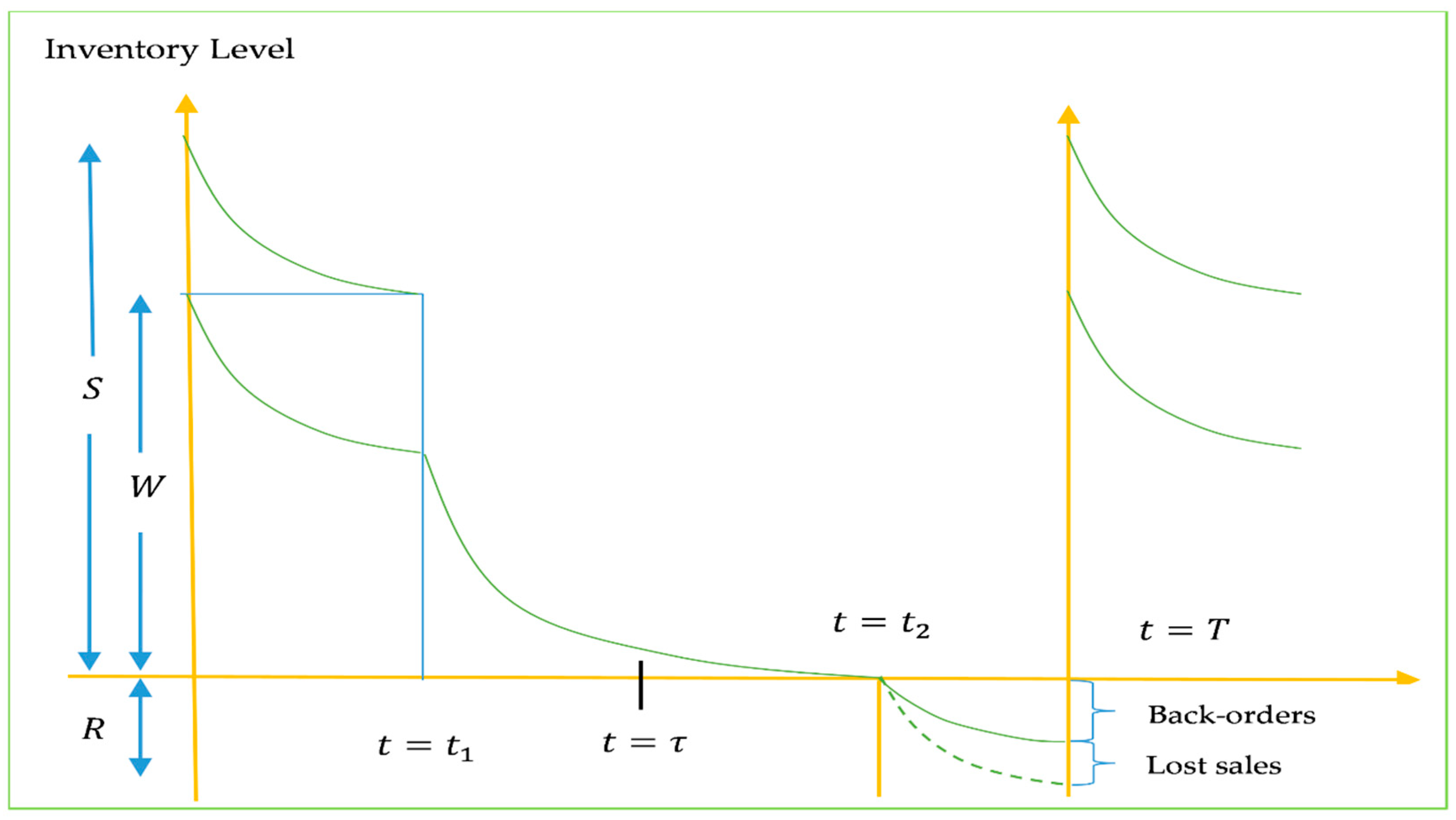
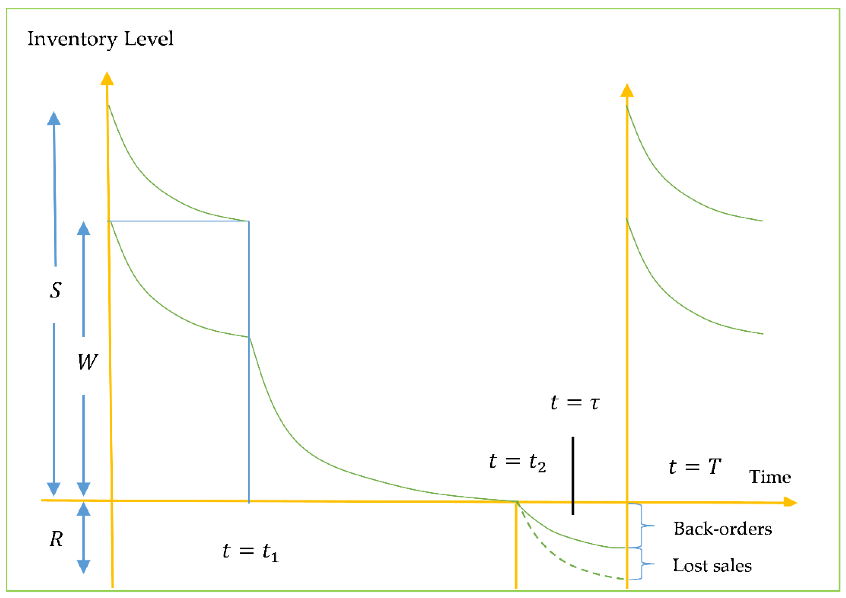
4. Mathematical Model

A retailer first orders Q = ( S + R ) units of a single deteriorating product, of which R units are to be used to satisfy the partially backlogged demand. Then, the inventory level changes to S units. W units are reserved in an O.W. out of S units, and the rest of the quantity ( S W ) of units are in an R.W. Due to the combined effect of customer demand and the deterioration effect, the stock level in an R.W. decreases in the time interval [ 0 ,   t 1 ] , and it finishes at time t = t 1 . On the other side, the stock level W in an O.W. declines in [ 0 , t 1 ] due to deterioration only and it declines in [ t 1 , t 2 ] due to the joined effects of demand and deterioration from customers, and it finishes at t = t 2 . Following that, shortages start to occur during the time [ t 2 ,   T ] , which accrue at a rate of 1 1 + δ T t depending on the waiting time length until the arrival of the new lot at time t = T . The total shortage that occurs in this period is R units. The primary objective is to determine the optimal values of t 1 , t 2 , T , and p to maximize the retailer’s profit per unit of time and obtain the corresponding Q values.

4.1. Inventory Model for Rented Warehouse (R.W.)

The inventory level in an R.W. ( 0 t t 1 ) declines due to the joint effect of demand and deterioration of the items, so it follows the following differential equation:
d I 1 ( t ) d t + θ I 1 t = D ( A , p ) ,                     0 t t 1
This is subject to the following conditions: I 1 0 = S W and I 1 t 1 = 0 .
By solving Equation (1) and using I 1 t 1 = 0 , one can obtain
I 1 t = D θ e θ t 1 t 1
Again, by using I 1 0 = S W 1 , in Equation (2), one can obtain the initial stock.
S = W + D θ e θ t 1 1

4.2. Inventory Model for Owned Warehouse (O.W.)

The inventory level of an O.W. can be determined from the following differential equation as
d I 2 ( t ) d t + η I 2 t = 0 ,               0 t t 1
d I 2 ( t ) d t + η I 2 t = D ( A , p ) ,                     t 1 < t t 2
d I 2 ( t ) d t = D A , p 1 + δ T t ,                       t 2 < t T
This is subject to the following conditions: I 2 0 = W , I 2 t 2 = 0 , and I 2 T = R . Using the given conditions, the solutions of Equations (4)–(6) are given by
I 2 t = W e η t ,       0 t t 1
I 2 t = D η e η t 2 t 1 ,       t 1 < t t 2
I 2 t = D δ log 1 + δ T t R ,       t 2 < t T
Also I 2 ( t ) is continuous at t = t 1 and t = t 2 . The continuity condition of I 2 t at time t = t 1 gives us
W e η t 1 = D η e η t 2 t 1 1
W = D η e η t 2 e η t 1
  t 2 = 1 η log e η t 1 + η W D
Also, from the continuity of I 2 t at time t = t 2 , we can obtain the maximum shortage level, which is calculated as
R = D δ log 1 + δ T t 2
Therefore, the initial lot size for the whole cycle is given as
Q = S + R = W + D θ e θ t 1 1 + D δ log 1 + δ T t 2
The total cycle length is obtained from Equation (12) as
T = t 2 + 1 δ e δ D Q W D θ e θ t 1 1 1

4.3. Computation of Different Costs

(i)
Cost of ordering (O.C.): K .
(ii)
Cost of advertisement (A.C.): c a A .
(iii)
Holding cost ( H . C . ) : The total cost of holding (H.C.) over a complete cycle is given by
H C = c i 0 t 1 g + h 1 t I 1 t d t + c i 0 t 2 g + h 2 t I 2 t d t
H C = c i D 2 θ 3 2 e θ t 1 θ t 1 1 g θ + h 1 h 1 θ 2 t 1 2 + c i η 2 η g W 1 e η t 1 + h 2 η t 1 1 e η t 1 + 1 + c i D η g η e η t 2 t 1 1 + h 2 η 2 1 + η t 1 e η t 2 t 1 1 η t 2 g t 2 t 1 1 2 h 2 t 2 2 t 1 2
(iv)
Shortage cost (S.C.):
S C = c s t 2 T I 2 t d t
S C = c s R T t 2 + D δ 2 δ T t 2 1 + δ T t 2 log 1 + δ T t 2
S C = C s D δ T t 2 1 δ log 1 + δ T t 2
(v)
Deterioration cost (D.C.):
D C = c d S W 0 t 1 D d t + c d W t 1 t 2 D d t = c d S D t 2
= c d W + D θ e θ t 1 1 D t 2
(vi)
Lost sale cost (LSC):
L S C = c l t 2 T 1 1 1 + δ T t D d t
= c l D T t 2 1 δ log 1 + δ T t 2
Therefore, the total cyclic cost except for the purchasing cost is
T C = O C + A C + H C + S C + D C + L S C
T C = K + C a A + c i D 2 θ 3 2 e θ t 1 θ t 1 1 g θ + h 1 h 1 θ 2 t 1 2 + c i η 2 η g W 1 e η t 1 + h 2 η t 1 1 e η t 1 + 1 + c i D η g η e η t 2 t 1 1 + h 2 η 2 1 + η t 1 e η t 2 t 1 1 η t 2 g t 2 t 1 1 2 h 2 t 2 2 t 1 2 + C l + C s δ D T t 2 1 δ log 1 + δ T t 2 + c d W 1 + D θ e θ t 1 1 D t 2

5. Analysis of Trade Credit Policy

The supplier gives their retailer the credit time τ their retailer. So, the two following situations could occur:
Section 5.1: When the trade credit time is in a stock-in period, i.e., ( 0 τ t 2 );
Section 5.2: When the trade credit time is in a stock-out period, i.e., ( t 2 τ T ).

5.1. When Trade Credit Time Is in Stock-In Period, i.e., ( 0 τ t 2 )

Figure 1 represents a schematic diagram for trade credit time is in stock in period. In this scenario, the retailers have to pay the total amount c i Q to the supplier at time t = τ . The retailer’s total accrued amount due to selling the product and the interest earned at time t = τ is given by
E 1 = p 0 τ D d t + p e 0 τ 0 t D d u d t + p R 1 + e τ
E 1 = p τ D 1 + 1 2 e τ + p R 1 + e τ
Based on the difference between the money E 1 and c i Q , there are two possibilities that may arise:
Section 5.1.1: When E 1 c i Q .
Section 5.1.2: When E 1 < c i Q .

5.1.1. When the Total Earning Amount Is Greater than the Total Purchasing Cost, i.e., E 1 c i Q

In this case, the total profit function Y 1 t 1 , t 2 , T for the retailer in a complete cycle [ 0 ,   T ] can be defined as follows:
Y 1 t 1 , t 2 , T = e x t r a   a m o u n t   a f t e r   p a y i n g   t h e   m a n u f a c t u r e r + i n t e r e s t   e a r n e d   f o r   e x t r a   a m o u n t   i n   t h e   p e r i o d τ , T + s a l e s   r e v e n u e   i n   t h e   p e r i o d τ , t 2 + i n t e r e s t   e a r n e d   f r o m   s a l e s   r e v e n u e   i n   t h e   p e r i o d τ ,   t 2 + i n t e r e s t   e a r n e d   i n   t h e   p e r i o d t 2 , T T C
Y 1 t 1 , t 2 , T = E 1 c i Q 1 + e T τ + p τ t 2 D d t + p e τ t 2 τ t D d u d t 1 + e T t 2 T C
= E 1 c i Q 1 + e T τ + p D t 2 τ + 1 2 p D e t 2 τ 2 1 + e T t 2 T C
= p τ D 1 + 1 2 e τ + p 1 + e τ D δ log 1 + δ T t 2 c i W + D θ e θ t 1 1 + D δ log 1 + δ T t 2 1 + e T τ + p D t 2 τ + 1 2 p D e t 2 τ 2 1 + e T t 2 K + C a A c i D 2 θ 3 2 e θ t 1 θ t 1 1 g θ + h 1 h 1 θ 2 t 1 2 c i η 2 η g W 1 e η t 1 + h 2 η t 1 1 e η t 1 + 1 c i D η g η e η t 2 t 1 1 + h 2 η 2 1 + η t 1 e η t 2 t 1 1 η t 2 g t 2 t 1 1 2 h 2 t 2 2 t 1 2 C l + C s δ D T t 2 1 δ log 1 + δ T t 2 c d W + D θ e θ t 1 1 D t 2
So, the optimization problem is
M a x i m i z e   Z 1 t 1 , t 2 , T = Y 1 t 1 , t 2 , T T S u b j e c t   t o   0 < τ t 1

5.1.2. When the Total Earning Amount Is Less than the Total Purchasing Cost, i.e., E 1 < c i Q

The total accrued amount at time t = τ in this subcase is less than the totalpurchasing cost. Once more, two situations could manifest at this point as follows:
When a partial payment is allowed at t = τ .
When a partial payment is not permitted at t = τ .

When a Partial Payment Is Allowed at t = τ

In this situation, the retailer pays E 1 amount to the supplier at time t = τ , and suppose that the remaining amount c i Q E 1 will be paid at time t = λ ( λ > τ ) . As a result, during the period [ τ ,   λ ] , the retailer must pay some interest at the rate, say, e 1 , on the amount of c i Q E 1 . At time t = λ , the retailer’s required amount is c i Q E 1 1 + e 1 λ τ .
T h e   t o t a l   a m o u n t   a c c r u e d   b y   t h e   r e t a i l e r   d u r i n g   t h e   t i m e   τ ,   λ = s a l e s   r e v e n u e   i n   t h e   t i m e   p e r i o d   τ , λ + i n t e r e s t   e a r n e d   f r o m   s a l e s   r e v e n u e   i n   t h e   t i m e   τ , λ = p τ λ D d t + p e τ λ τ t D d u d t = p D λ τ + 1 2 p D e λ τ 2
Hence, at time t = λ , the required amount is equal to the accrued amount of the retailer, i.e.,
c i Q E 1 1 + e 1 λ τ = p D λ τ + 1 2 p D e λ τ 2
Therefore, the total profit for the whole inventory cycle is given by
Y 2 t 1 , t 2 , T = s a l e s   r e v e n u e   i n   t h e   t i m e   p e r i o d   λ , t 2 + i n t e r e s t   e a r n e d   f r o m   s a l e s   r e v e n u e   i n   t h e   t i m e   p e r i o d   λ ,   t 2 + i n t e r e s t   e a r n e d   i n   t h e   t i m e   p e r i o d   t 2 , T T C
Y 2 t 1 , t 2 , T = p λ t 2 D d t + p e λ t 2 λ t D d u d t 1 + e T t 2 T C
Y 2 t 1 , t 2 , T = p D t 2 λ + 1 2 p e D t 2 λ 2 1 + e T t 2 T C  
Y 2 t 1 , t 2 , T = p D t 2 λ + 1 2 p e D t 2 λ 2 1 + e T t 2 K + C a A c i D 2 θ 3 2 e θ t 1 θ t 1 1 g θ + h 1 h 1 θ 2 t 1 2 c i η 2 η g W 1 e η t 1 + h 2 η t 1 1 e η t 1 + 1 c i D η g η e η t 2 t 1 1 + h 2 η 2 1 + η t 1 e η t 2 t 1 1 η t 2 g t 2 t 1 1 2 h 2 t 2 2 t 1 2 C l + C s δ D T t 2 1 δ log 1 + δ T t 2 c d W + D θ e θ t 1 1 D t 2
Therefore, the optimization problem is
M a x i m i z e   Z 2 t 1 ,   t 2 , T = Y 2 t 1 , t 2 , T T S u b j e c t   t o   ( 16 )   a n d   0 < τ t 2 < T

When a Partial Payment Is Not Allowed at t = τ

Here, the retailers must pay the total credit amount to the supplier at λ   ( λ > τ ) . So, the retailers must pay the interest of the total credited amount for the period [ τ , λ ] .
Hence, at time t = λ , the required amount is equal to the accrued amount of the retailer, i.e.,
c i Q 1 + e 1 λ τ = p 0 λ D d t + p e 0 λ 0 t D d u d t + p R 1 + e λ
c i Q 1 + e 1 λ τ = p D λ 1 + 1 2 e λ + p R 1 + e λ
Therefore, the total profit for the whole inventory cycle is given by
Y 3 t 1 ,   t 2 , T = s a l e s   r e v e n u e   i n   t h e   p e r i o d   λ , t 2 + i n t e r e s t   e a r n e d   f r o m   s a l e s   r e v e n u e   i n   t h e   p e r i o d   λ ,   t 2 + i n t e r e s t   e a r n e d   i n   t h e   p e r i o d   t 2 , T T C
= p λ t 2 D d t + p e λ t 2 λ t D d u d t 1 + e T t 2 T C
= p D t 2 λ + 1 2 p e D t 2 λ 2 1 + e T t 2 T C
= p D t 2 λ + 1 2 p e D t 2 λ 2 1 + e T t 2 K + C a A c i D 2 θ 3 2 e θ t 1 θ t 1 1 g θ + h 1 h 1 θ 2 t 1 2 c i η 2 η g W 1 e η t 1 + h 2 η t 1 1 e η t 1 + 1 c i D η g η e η t 2 t 1 1 + h 2 η 2 1 + η t 1 e η t 2 t 1 1 η t 2 g t 2 t 1 1 2 h 2 t 2 2 t 1 2 C l + C s δ D T t 2 1 δ log 1 + δ T t 2 c d W + D θ e θ t 1 1 D t 2
So, the optimization problem is
M a x i m i z e   Z 3 t 1 ,   t 2 , T = Y 3 t 1 , t 2 , T T   S u b j e c t   t o   18   a n d   0 < τ t 2 < T

5.2. When Trade Credit Time Is in a Stock-Out Period, i.e., ( t 2 τ T )

Figure 2 represents a schematic diagram for trade credit time is in stock out period. Here, the retailers accrue the sales revenue by selling products, and interest is earned by investing the selling amount to the bank or any other organization. The total sales revenue of the retailer up to time t = τ is given by
E 2 = p 0 t 2 D d t + p e 0 t 2 0 t D d u d t 1 + e τ t 2 + p R 1 + e τ
= p D t 2 + 1 2 p e D t 2 2 1 + e τ t 2 + p R 1 + e τ
Therefore, the total profit for an entire cycle is given by
Y 4 t 1 ,   t 2 , T = r e s t   a m o u n t + i n t e r e s t   e a r n e d   f r o m   r e s t   a m o u n t   i n   t h e   t i m e   τ , T T C
= E 2 c i Q 1 + e T τ T C
{ p D t 2 + 1 2 p e D t 2 2 1 + e τ t 2 + p 1 + e τ D δ log 1 + δ T t 2 c i W + D θ e θ t 1 1 + D δ log 1 + δ T t 2 } 1 + e T τ K + C a A c i D 2 θ 3 2 e θ t 1 θ t 1 1 g θ + h 1 h 1 θ 2 t 1 2 c i η 2 η g W 1 1 e η t 1 + h 2 η t 1 1 e η t 1 + 1 c i D η g η e η t 2 t 1 1 + h 2 η 2 1 + η t 1 e η t 2 t 1 1 η t 2 g t 2 t 1 1 2 h 2 t 2 2 t 1 2 c l + c s δ D T t 2 1 δ log 1 + δ T t 2 c d W + D θ e θ t 1 1 D t 2
Therefore, the optimization problem is
M a x i m i z e   Z 4 t 1 ,   t 2 , T = Y 4 t 1 , t 2 , T T S u b j e c t   t o   0 < τ t 2 < T

6. Computational Algorithms

In this section, we obtain the conditions for the existence of the optimal solution for four different objective functions described in Section 5.

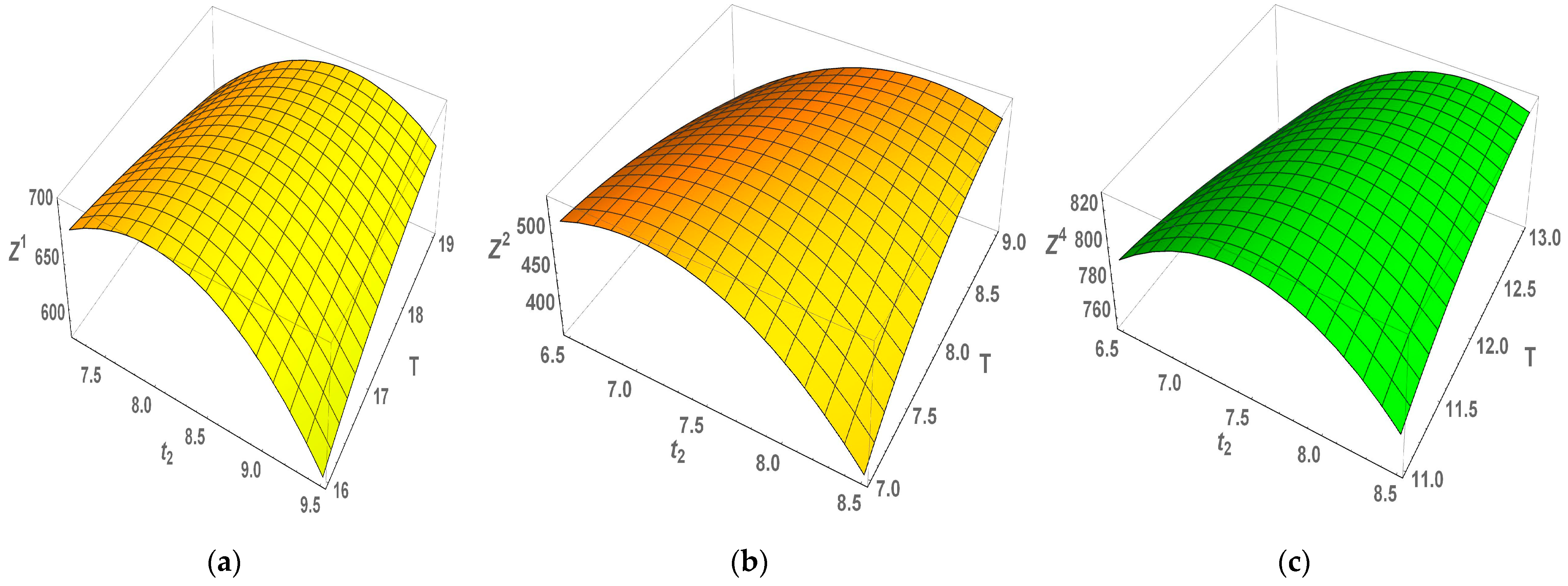
6.1. Conditions for the Existence of Optimal Solution of Z 1 t 1 , t 2 , T

Here, we calculated the first-order partial derivatives of Z 1 t 1 , t 2 , T w.r.t t 1 , t 2 , and T , respectively, and then set them as being equal to zero.
Z 1 t 1 = 1 T [ c i D e θ t 1 1 + e T τ c i D 2 θ 2 2 e θ t 1 1 g θ + h 1 2 h 1 θ t 1 c i η η g W e η t 1 + h 2 e η t 1 2 η t 1 c i D η g + h 2 t 1 1 e η t 2 t 1 c d D e θ t 1 ] = 0
c i D e θ t 1 1 + e T τ + c i D 2 θ 2 2 e θ t 1 1 g θ + h 1 2 h 1 θ t 1 + c i η η g W e η t 1 + h 2 e η t 1 2 η t 1 + c i D η g + h 2 t 1 1 e η t 2 t 1 + c d D e θ t 1 = 0
and
Z 1 t 2 = 1 T [ p 1 + e τ c i 1 + e T τ D 1 + δ T t 2 + p D 1 + e t 2 τ 1 + e T t 2 e p D t 2 τ + 1 2 e t 2 τ 2 c i D η g e η t 2 t 1 + h 2 η 1 + η t 1 e η t 2 t 1 1 g h 2 t 2 + C l + C s δ D δ 1 + δ T t 2 + c d D ] = 0
c i p 1 + e τ 1 + e T τ D 1 + δ T t 2 + p D 1 + e t 2 τ 1 + e T t 2 e p D t 2 τ + 1 2 e t 2 τ 2 c i D η g e η t 2 t 1 + h 2 η 1 + η t 1 e η t 2 t 1 1 g h 2 t 2 + C l + C s δ D δ 1 + δ T t 2 + c d D = 0
and
Z 1 T = 1 T 2 { T [ p 1 + e τ c i 1 + e T τ D 1 + δ T t 2 + e { p τ D 1 + 1 2 e τ + p 1 + e τ D δ log 1 + δ T t 2 c i W + D θ e θ t 1 1 + D δ log 1 + δ T t 2 } + e p D t 2 τ + 1 2 e t 2 τ 2 C l + C s δ D δ 1 + δ T t 2 ] Z 1 t 1 , t 2 , T } = 0
p 1 + e τ c i 1 + e T τ D T 1 + δ T t 2 + e τ 1 { p τ D 1 + 1 2 e τ + p 1 + e τ D δ log 1 + δ T t 2 c i W + D θ e θ t 1 1 + D δ log 1 + δ T t 2 } + e t 2 1 p D t 2 τ + 1 2 e t 2 τ 2 C l + C s δ δ D T 1 + δ T t 2 + K + C a A + c i D 2 θ 3 2 e θ t 1 θ t 1 1 g θ + h 1 h 1 θ 2 t 1 2 + c i η 2 η g W 1 e η t 1 + h 2 η t 1 1 e η t 1 + 1 + c i D η g η e η t 2 t 1 1 + h 2 η 2 1 + η t 1 e η t 2 t 1 1 η t 2 g t 2 t 1 1 2 h 2 t 2 2 t 1 2 + C l + C s δ D T t 2 1 δ log 1 + δ T t 2 + c d W + D θ e θ t 1 1 + D t 2 = 0
The concavity of the function Z 1 t 1 , t 2 , T can be checked by using the Hessian matrix ( H ) as follows:
H = 2 Z 1 t 1 2 2 Z 1 t 1 t 2 2 Z 1 t 1 T 2 Z 1 t 2 t 1 2 Z 1 t 2 2 2 Z 1 t 2 T 2 Z 1 T t 1 2 Z 1 T t 2 2 Z 1 T 2
The profit function Z 1 t 1 , t 2 ,   T will be the maximum for the values of t 1 , t 2 ,   T , if all of the principal determinants of the Hessian matrix satisfy the following conditions at t 1 , t 2 ,   T as
H 11 1 = 2 Z 1 t 1 2 < 0 , H 22 1 = 2 Z 1 t 1 2 2 Z 1 t 2 2 2 Z 1 t 2 t 1 2 Z 1 t 1 t 2 > 0 , H 33 1 = H < 0 .
Due to the high nonlinearity of the Hessian matrix, closed-form analytical proof is challenging to obtain. So, we alternated a numerical analysis to verify the concavity of Z 1 t 1 , t 2 , T .

6.2. Conditions for the Existence of Optimal Solution of Z 2 t 1 , t 2 , T

Here, we calculated the first-order partial derivatives of Z 2 t 1 , t 2 , T w.r.t t 1 , t 2 , and T , respectively, and then set them as being equal to zero.
Z 2 t 1 = 1 T [ c i D 2 θ 2 2 e θ t 1 1 g θ + h 1 2 h 1 θ t 1 c i η η g W e η t 1 + h 2 e η t 1 2 η t 1 c i D η g + h 2 t 1 1 e η t 2 t 1 c d D e θ t 1 ] = 0
c i D 2 θ 2 2 e θ t 1 1 g θ + h 1 2 h 1 θ t 1 + c i η η g W e η t 1 + h 2 e η t 1 2 η t 1 + c i D η g + h 2 t 1 1 e η t 2 t 1 + c d D e θ t 1 = 0
and
Z 2 t 2 = 1 T [ p D 1 + e t 2 λ 1 + e T t 2 e p D t 2 λ + 1 2 e t 2 λ 2 c i D η g e η t 2 t 1 + h 2 η 1 + η t 1 e η t 2 t 1 1 g h 2 t 2 + C l + C s δ D δ 1 + δ T t 2 + c d D ] = 0
p D 1 + e t 2 λ 1 + e T t 2 e p D t 2 λ + 1 2 e t 2 λ 2 c i D η g e η t 2 t 1 + h 2 η 1 + η t 1 e η t 2 t 1 1 g h 2 t 2 + C l + C s δ D δ 1 + δ T t 2 + c d D = 0
and
Z 2 T = 1 T 2 T e p D t 2 λ + 1 2 e t 2 λ 2 C l + C s δ D δ 1 + δ T t 2 Z 1 t 1 , t 2 , T = 0
e t 2 1 p D t 2 λ + 1 2 e t 2 λ 2 C l + C s δ δ D T 1 + δ T t 2 + K + C a A + c i D 2 θ 3 2 e θ t 1 θ t 1 1 g θ + h 1 h 1 θ 2 t 1 2 + c i η 2 η g W 1 e η t 1 + h 2 η t 1 1 e η t 1 + 1 + c i D η g η e η t 2 t 1 1 + h 2 η 2 1 + η t 1 e η t 2 t 1 1 η t 2 g t 2 t 1 1 2 h 2 t 2 2 t 1 2 + C l + C s δ D T t 2 1 δ log 1 + δ T t 2 + c d W + D θ e θ t 1 1 + D t 2 = 0
As in Section 6.1, we verified the concavity of Z 2 t 1 , t 2 , T numerically with the help of the Hessian matrix.

6.3. Conditions for the Existence of Optimal Solution of Z 3 t 1 , t 2 , T

Since the objective function Z 3 t 1 , t 2 , T is the same as Z 2 t 1 , t 2 , T , the existence conditions of the optimal solution of Z 3 t 1 , t 2 , T is the same as those in Section 6.2.

6.4. Conditions for the Existence of Optimal Solution of Z 4 t 1 , t 2 , T

Here, we calculated the first-order partial derivatives of Z 1 t 1 , t 2 , T w.r.t t 1 , t 2 , and T , respectively, and then set them as being equal to zero.
Z 4 t 1 = 1 T [ c i D e θ t 1 1 + e T τ c i D 2 θ 2 2 e θ t 1 1 g θ + h 1 2 h 1 θ t 1 c i η η g W e η t 1 + h 2 e η t 1 2 η t 1 c i D η g + h 2 t 1 1 e η t 2 t 1 c d D e θ t 1 ] = 0
c i D e θ t 1 1 + e T τ + c i D 2 θ 2 2 e θ t 1 1 g θ + h 1 2 h 1 θ t 1 + c i η η g W e η t 1 + h 2 e η t 1 2 η t 1 + c i D η g + h 2 t 1 1 e η t 2 t 1 + c d D e θ t 1 = 0
and
Z 4 t 2 = 1 T { 1 + e T τ p D 1 + e t 2 1 + e τ t 2 e p D t 2 + 1 2 e t 2 2 + c i p 1 + e τ D 1 + δ T t 2 c i D η g e η t 2 t 1 + h 2 η 1 + η t 1 e η t 2 t 1 1 g h 2 t 2 + C l + C s δ D δ 1 + δ T t 2 + c d D } = 0
1 + e T τ p D 1 + e t 2 1 + e τ t 2 e p D t 2 + 1 2 e t 2 2 + c i p 1 + e τ D 1 + δ T t 2 c i D η g e η t 2 t 1 + h 2 η 1 + η t 1 e η t 2 t 1 1 g h 2 t 2 + C l + C s δ D δ 1 + δ T t 2 + c d D = 0
and
Z 4 T = 1 T 2 { T [ p 1 + e τ c i 1 + e T τ D 1 + δ T t 2 + e { p D t 2 + 1 2 p e D t 2 2 1 + e τ t 2 + p 1 + e τ D δ log 1 + δ T t 2 c i W + D θ e θ t 1 1 + D δ log 1 + δ T t 2 } C l + C s δ D δ 1 + δ T t 2 ] Z 4 t 1 , t 2 , T } = 0
p 1 + e τ c i 1 + e T τ D T 1 + δ T t 2 + e τ 1 { p D t 2 + 1 2 p e D t 2 2 1 + e τ t 2 + p 1 + e τ D δ log 1 + δ T t 2 c i W + D θ e θ t 1 1 + D δ log 1 + δ T t 2 } C l + C s δ δ D T 1 + δ T t 2 + K + C a A + c i D 2 θ 3 2 e θ t 1 θ t 1 1 g θ + h 1 h 1 θ 2 t 1 2 + c i η 2 η g W 1 e η t 1 + h 2 η t 1 1 e η t 1 + 1 + c i D η g η e η t 2 t 1 1 + h 2 η 2 1 + η t 1 e η t 2 t 1 1 η t 2 g t 2 t 1 1 2 h 2 t 2 2 t 1 2 + C l + C s δ D T t 2 1 δ log 1 + δ T t 2 + c d W + D θ e θ t 1 1 + D t 2 = 0
As in Section 6.1, we verified the concavity of Z 4 t 1 , t 2 , T numerically with the help of the Hessian matrix.

7. Numerical Simulation

In this section, we perform the numerical optimization of the proposed models discussed in the earlier sections. To obtain the numerical and graphical outcomes in this section, we used the Wolfram Mathematica 11 software.

7.1. Solution Procedure

In this subsection, we discuss the computational process of the above-described optimization problems. Considering the all-unit price discount policy, we designed the Algorithm 1 to compute the optimal solutions to maximize the total profit. Algorithm 1 is suitable for all of the above-described optimization problems.
Algorithm 1: Numerical computation procedure for getting best profit
Step   1 :   Input   all   of   the   given   values   of   the   parameters K , a , b , g , h 1 , h 2 , p , θ , η , c s , c l , c d , W , τ , λ , e , e 1 , δ , c a , A , γ .
Step   2 :   Set   i = m   and   Z m a x = 0 .
Step   3 :   Input   the   given   value   of   c m   and   solve   the   equations   Z t 1 = 0 ,   Z t 2 = 0 ,   and   Z T = 0 for   t 1 ,   t 2 ,   and   T .   Calculate   the   order   quantity   Q   using   t 1 ,   t 2 ,   and   T   from   ( 12 ) .
Step   4 :   If   Q   does   not   belong   to   the   correct   quantity   break   q m Q < q m + 1 , this solution
is infeasible, so go to step 7. Otherwise, go to step 5.
Step   5 :   If   Q   belongs   to   the   correct   quantity   break   q m Q < q m + 1 , the solution is
feasible .   Calculate   Z i .   If   Z i > Z m a x ,   set   Z m a x = Z i . Go to step 6.
Step   6 :   Check   the   concavity   conditions   of   Z   through   the   Hessian   matrix ,   i . e . ,   H 11 < 0 ,
H 22 > 0 ,   and   H 33 < 0 . If this condition holds, go to step 8. Otherwise, go to step 7.
Step   7 :   If   i 2 ,   set   i = i 1   and   go   to   step   2 .   If   i = 1 , go to step 8.
Step   8 :   The   final   solution   is   obtained .   The   total   average   profit   is   Z m a x with the optimal
values of   t 1 ,   t 2 T ,   S ,   R ,   and   Q .
Step 9: End.

7.2. Numerical Illustration

Example 1.
Consider the situation when the trade credit time is in the stock-in period and the sales revenue is more significant than the purchasing cost, and suppose that the supplier offers the quantity discount to the retailer as per Table 3.
Also suppose K = 250 ,   a = 100 ,   b = 2.5 ,   g = 0.2 ,   h 1 = 0.6 ,   h 2 = 0.2 ,   p = 20 , θ = 0.05 , η = 0.20 ,   c s = 6.5 ,   c l = 0.5 ,   c d = 0.9 ,   W = 300 ,   τ = 0.5 ,   e = 0.09 ,   δ = 0.06 ,   c a = 15 ,   A = 4 , a n d   γ = 0.03 .   To   compute   the   optimal   result ,   follow   the   following   steps :
Step 1: Initially set Z m a x 1 = 0 and i = 3 .
Iteration 1: i = 3 .
Step 2: c 3 = 4.90 1000 Q < .
By solving Equations (21)–(23) we obtain t 1 = 3.42237 , t 2 = 8.77695 , and T = 18.9512 , and the order quantity, which is obtained from (12), is Q = 913.543 . Using these values, the total average profit from Equation (15) is Z 3 1 = 724.571 . As Q does not lie in the quantity break 1000 Q < , this solution is not feasible, so go to step 3.
Step 3: Set i = 2 and go to step 4.
Iteration 2: i = 2 .
Step 4: c 2 = 5 ( 500 Q < 1000 ) .
By substituting the value of c 2 in Equations (21)–(23) and by solving them, we obtain   t 1 = 3.10444 , t 2 = 8.31027 , and T = 17.5875 . The lot size obtained from (12) is Q = 863.239 . Using these values, the total average profit from Equation (15) is Z 2 1 = 702.89 . Since Q lies in the quantity break ( 500 Q < 1000 ) , this solution is feasible, and Z 2 1 = 702.89 > Z m a x 1 = 0 . Therefore, Z m a x 1 = 702.89 . Go to step 5.
Step 5: The Hessian matrix’s principal minors are H 11 1 = 41.3547 < 0 , H 22 1 = 2166.49 > 0 and H 33 1 = 1133.35 < 0 . Therefore, the concavity conditions of the objective function are satisfied.
Step 6: Final solution.
Therefore, the optimal solution is t 1 * = 3.10444 , t 2 * = 8.31027 , T * = 17.5875 , S * = 476.224 , R * = 387.015 , Q * = 863.239 , and Z m a x 1 = 702.89 . The concave nature of the profit function against t 2 and T is visualized in Figure 3a.
Example 2.
Consider the situation when the trade credit time is in the stock-in period, and the sales revenue is less than the purchasing cost; meanwhile, the supplier allows for a partial payment. Suppose that the supplier offers the quantity discount as in Example 1, taking λ = 1.5 , h 1 = 0.3 , h 2 = 0.1 , and other inputs the same way as in Example 1. To compute the optimal result, follow the following steps:
Step 1: Initially set Z m a x 2 = 0 and i = 3 .
Iteration 1: i = 3 .
Step 2: c 3 = 4.90 1000 Q < .
By solving Equations (24)–(26), we obtain t 1 = 3.56916 , t 2 = 7.71561 , and T = 8.32148 , and the ordering quantity, which is obtained from (12), is Q = 536.2649 . Using these values, the total average profit from Equation (17) is Z 3 2 = 550.964 . As Q does not lie in the quantity break 1000 Q < , this solution is not feasible, so go to step 3.
Step 3: Put i = 2 and go to step 4.
Iteration 2: i = 2 .
Step 4: c 2 = 5 ( 500 Q < 1000 ) .
By substituting the value of c 2 in Equations (24)–(26) and by solving, we obtain t 1 = 3.50899 , t 2 = 7.62086 , and T = 8.21176 . The lot size obtained from (12) is Q = 531.7382 . Using these values, the total average profit from Equation (17) is Z 2 2 = 541.829 . Since Q lies in the quantity break ( 500 Q < 1000 ) , this solution is feasible, and Z 2 2 = 541.829 > Z m a x 2 = 0 . Therefore, Z m a x 2 = 541.829 . Go to step 5.
Step 5: The Hessian matrix’s principal minors are H 11 2 = 60.708 < 0 , H 22 2 = 5857.68 > 0 and H 33 2 = 32411.5 < 0 . Therefore, the concavity conditions of the objective function are satisfied.
Step 6: Final solution.
Therefore, the optimal solution is t 1 * = 3.50899 , t 2 * = 7.62086 , T * = 8.21176 , S * = 501.269 , R * = 30.4692 , Q * = 531.738 , and Z m a x 2 = 541.829 . The concave nature of the profit function ( Z 2 ) against t 2 and T is visualized in Figure 3b.
Example 3.
Consider that the trade credit time is in a stock-out period, and the sales revenue is more significant than the purchasing cost. Suppose that the supplier offers a quantity discount as in Example 1 along with τ = 7.75 , h 1 = 0.10 , h 2 = 0.05 , and e = 0.06 , and the other inputs are the same as in Example 1.
Step 1: Initially set Z m a x 4 = 0 and i = 3 .
Iteration 1: i = 3 .
Step 2: c 3 = 4.90 1000 Q < .
By solving Equations (27)–(29), we obtain t 1 = 2.28268 , t 2 = 7.750 , and T = 12.3151 , and the order quantity obtained from (12) is Q = 638.603 . Using these values, the total average profit from Equation (20) is Z 3 4 = 838.36 . As Q does not lie in the quantity break 1000 Q < , this solution is not feasible, so go to step 3.
Step 3: Put i = 2 and go to step 4.
Iteration 2: i = 2 .
Step 4: c 2 = 5 ( 500 Q < 1000 ) . By substituting the value of c 2 in Equations (27)–(29) and by solving, we obtain t 1 = 2.28627 , t 2 = 7.750 , and T = 12.3313 . The order size obtained from (12) is Q = 639.481 . Using these values, the total average profit from Equation (20) is Z 2 4 = 826.775 . Since Q lies in the quantity break ( 500 Q < 1000 ) , this solution is feasible, and Z 2 4 = 826.775 > Z m a x 4 = 0 . Therefore, Z m a x 4 = 826.775 ; go to step 5.
Step 5: The Hessian matrix’s principal minors are H 11 4 = 17.9467 < 0 , H 22 4 = 769.038 > 0 , and H 33 4 = 2504.08 < 0 . Therefore, the concavity conditions of the objective function are satisfied.
Step 6: Final solution.
Therefore, the optimal solution is t 1 * = 2.28627 , t 2 * = 7.750 , T * = 12.3313 , S * = 427.095 , R * = 212.386 , Q * = 639.48 , and Z m a x 2 = 826.775 . The concave nature of the profit function ( Z 2 ) against t 2 and T is visualized in Figure 3c.

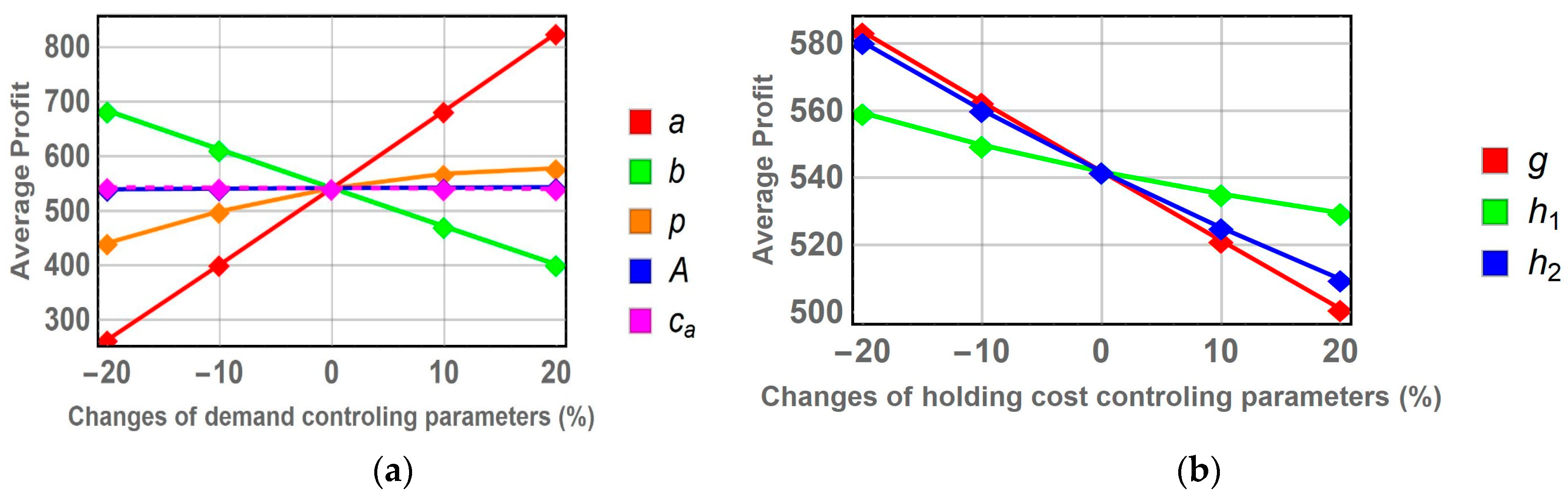
8. Sensitivity Analysis and Managerial Insights

8.1. Sensitivity of the Optimal Solution

Here, we examined the effects of various input parameters on the optimal solutions, such as the total cycle duration ( T ) , lot size ( Q ) , and total profit of the whole inventory cycle; we carried out a sensitivity analysis of example 2. This analysis changed one parameter’s value from +20% to −20% at a time, with the other parameters remaining fixed at their starting levels. The modifications made to the optimal values are presented in Table 4. Figure 4 also shows the sensitivity of the optimal results in a graphical manner.
Table 4 and Figure 4 together perceive the following points regarding the optimal decision:
Observation 1: The time t 1 * at which the inventory level in an R.W. finishes is positively dependent on the parameters K , b , p , A , c a , and η positively, whereas t 1 * is dependent on a , γ , g , h 1 , h 2 , θ , c s , c l , c d , and δ in a negative way.
Observation 2: The active retailing cycle time t 2 * increases when the values of the parameters K , b , p , A , and c a are increasing, and it increases when the values of the parameters a , γ , g , h 1 , h 2 , θ , η , c s , c l , c d , and δ are decreasing.
Observation 3: The total inventory cycle length T * is dependent on the parameters K , b , p , A , c a , and g in a positive way, and it is dependent on a , γ , h 1 , h 2 , θ , η , c s , c l , c d , and δ in a negative way.
Observation 4: The optimal order quantity Q * is dependent on the parameters K , a , p , A , c a , γ , g , η , c d , and δ in a positive manner; meanwhile, Q * is dependent on b , h 1 , h 2 , θ , c s , and c l in a negative manner.
Observation 5: The total average profit Z * is dependent on the parameters a , p , A , γ , and δ in a positive way, and it is dependent on K , b , c a , g , h 1 , h 2 , θ , η , c s , c l , and c d in a negative way.

8.2. Management Insights

The following managerial implications are driven by decoding the above observations:
Insight 1:   t 1 * is the optimal time cycle for storing inventory in a rented warehouse. Observation 1 implies that when the replenishment cost increases, rented warehousing continues. The renting tenure should be prolonged when demand is hiked through the promotion of products. Another managerial implication is that rented warehousing should be continued when deterioration in the warehouse increases. On the contrary, the tenure of the renting should be diminished while the rent warehouse’s decline increases. Also, the renting cycle should be shortened when the carrying costs due to both warehousing facilities improve.
Insight 2: t 2 * is the optimal retailing cycle. Observation 2 implies that the active retail process should be prolonged when the replenishment cost increases to avoid repeated replenishment. The demand hike through product promotion favors the broadened retail cycle to ensure optimal profitability. On the other hand, a rise in deterioration and carrying costs for different warehouses advocates diminishing the active retail process. The same managerial implications are derived for the whole decision cycle.
Insight 3: The optimal order size should be enhanced when demand is hiked through product promotion. The selling price enhancement also urges the big order size to ensure profit in a superior retail phenomenon. However, the carrying costs increase as time passes, so the order size should be reduced to prevent additional costs when continuing a large inventory lot.
Insight 4: The hike in demand potentially favors the profit enhancement goal. Interestingly, though a price hike is a barrier to creating demand, it can increase profitability, suppressing the demand diminishment. Also, the product’s advertisement favors the demand and average profit simultaneously. Deterioration and any costs during the retail cycle hinder the profit goal.

9. Conclusions and Future Research Directions

This work describes a unique inventory control model for the best possible warehousing decision-making situations. Several aspects emerge at the end of the analysis as a response to the research concerns on which this research was developed. First, boosting the selling price may assist in maximizing the average profit while avoiding the adverse effects of price increases on demand trends. Second, the advertisement frequency shows a positive impact on demand and average profit simultaneously. Third, the inventory carrying cost very strongly impacts decision making, leading to a diminishing order size to reduce cost. However, a big order size is advocated by demand enhancement through effective pricing and promotion. Fourth, rented warehouses can be used only when demand increases through pricing and promotion when product deterioration is minimized.
The suggested model encompasses several well-known inventory models as particular cases, which is a critical addition to this paper. Furthermore, this paper contributes an analytical approach to optimizing the proposed model, which took a lot of work to tackle with a complicated model with a reliable hypothesis. Also, this study’s numerical results bring some significant management insights. These are the merits of this present study. However, this current study has some limitations. The main demerit of this paper is that the numerical simulation was conducted for artificial data. Though the data were adjusted and validated according to the constraints raised in the analytical discussion, it would be error-free if the data were collected from real-world retail bodies.
The proposed model can be extended by incorporating the inventory size dependency of the demand rate in the model. The present model acknowledges the deterioration of products. Therefore, preservation means and their implications on managerial decisions may be a future research scope. Also, the proposed model can be viewed in uncertain decision phenomena, memory, learning censored decision phenomena, etc.

Author Contributions

Conceptualization, A.F.M., M.R. and R.H.; Methodology, A.F.M., R.H. and S.P.M.; Writing, M.R., R.H. and S.P.M.; Software and formal analysis, R.H. and M.R.; Validation, A.F.M., M.R. and S.P.M.; Resources and Supervision, A.F.M. and S.P.M.; Visualization, A.F.M., M.R. and R.H.; Review and Editing, A.F.M., M.R. and S.P.M.; Funding acquisition, A.F.M. All authors have read and agreed to the published version of the manuscript.

Funding

This study is supported via funding from Prince Sattam bin Abdulaziz University project number PSAU/2023/R/1445.

Institutional Review Board Statement

Not applicable.

Informed Consent Statement

Not applicable.

Data Availability Statement

The data used for the analysis are in the article.

Acknowledgments

The authors are very grateful to all the reviewers and journals editor for accepting the article.

Conflicts of Interest

The authors declare that there are no conflict of interest in this study.

References

  1. Harris, F.W. How many parts to make at once. J. Manuf. Syst. 1913, 10, 135–136. [Google Scholar] [CrossRef]
  2. Silver, E.A. A heuristic for selecting lot size quantities for the case of a deterministic time-varying demand rate and discrete opportunities for replenishment. Prod. Inventory Manag. J. 1973, 2, 64–74. [Google Scholar]
  3. Kim, J.; Hwang, H.; Shinn, S. An optimal credit policy to increase supplier’s profits with price-dependent demand functions. Prod. Plan. Control 1995, 6, 45–50. [Google Scholar] [CrossRef]
  4. Giri, B.C.; Pal, S.; Goswami, A.; Chaudhuri, K.S. An inventory model for deteriorating items with stock-dependent demand rate. Eur. J. Oper. Res. 1996, 95, 604–610. [Google Scholar] [CrossRef]
  5. Goyal, S.K.; Gunasekaran, A. An integrated production-inventory-marketing model for deteriorating items. Comput. Ind. Eng. 1995, 28, 755–762. [Google Scholar] [CrossRef]
  6. Nouira, I.; Frein, Y.; Hadj-Alouane, A.B. Optimization of manufacturing systems under environmental considerations for a greenness-dependent demand. Int. J. Prod. Econ. 2014, 150, 188–198. [Google Scholar] [CrossRef]
  7. Yang, Y.; Chi, H.; Zhou, W.; Fan, T.; Piramuthu, S. Deterioration control decision support for perishable inventory management. Decis. Support Syst. 2020, 134, 113308. [Google Scholar] [CrossRef]
  8. Rahman, M.S.; Manna, A.K.; Shaikh, A.A.; Konstantaras, I.; Bhunia, A.K. Optimal decision making, using interval uncertainty techniques, of a production-inventory model under warranty-linked demand and carbon tax regulations. Soft Comput. 2023, 27, 2903–2920. [Google Scholar] [CrossRef]
  9. Mondal, B.; Bhunia, A.K.; Maiti, M. Inventory models for defective items incorporating marketing decisions with variable production cost. Appl. Math. Model. 2009, 33, 2845–2852. [Google Scholar] [CrossRef]
  10. Muhlemann, A.P.; Valtis-Spanopoulos, N.P. A variable holding cost rate EOQ model. Eur. J. Oper. Res. 1980, 4, 132–135. [Google Scholar] [CrossRef]
  11. Sarker, B.R.; Jamal, A.M.M.; Wang, S. Optimal payment time under permissible delay in payment for products with deterioration. Prod. Plan. Control. 2000, 11, 380–390. [Google Scholar] [CrossRef]
  12. Aggarwal, S.P.; Jaggi, C.K. Ordering policies of deteriorating items under permissible delay in payments. J. Oper. Res. Soc. 1995, 46, 658–662. [Google Scholar] [CrossRef]
  13. Ho, C.H. The optimal integrated inventory policy with price-and-credit-linked demand under two-level trade credit. Comput. Ind. Eng. 2011, 60, 117–126. [Google Scholar] [CrossRef]
  14. Chen, L.H.; Kang, F.S. Integrated inventory models considering the two-level trade credit policy and a price-negotiation scheme. Eur. J. Oper. Res. 2010, 205, 47–58. [Google Scholar] [CrossRef]
  15. Shah, N.H.; Soni, H.N.; Patel, K.A. Optimizing inventory and marketing policy for non-instantaneous deteriorating items with generalized type deterioration and holding cost rates. Omega 2013, 41, 421–430. [Google Scholar] [CrossRef]
  16. Bhunia, A.K.; Shaikh, A.A.; Sharma, G.; Pareek, S. A two-storage inventory model for deteriorating items with variable demand and partial backlogging. J. Ind. Prod. Eng. 2015, 32, 263–272. [Google Scholar] [CrossRef]
  17. Jaggi, C.K.; Gautam, P.; Khanna, A. Inventory decisions for imperfect quality deteriorating items with exponential declining demand under trade credit and partially backlogged shortages. Qual. IT Bus. Oper. 2018, 18, 213–229. [Google Scholar]
  18. Tripathi, R.P. Innovation of economic order quantity (EOQ) model for deteriorating items with time-linked quadratic demand under non-decreasing shortages. Int. J. Appl. Comput. 2019, 5, 123. [Google Scholar] [CrossRef]
  19. Namdeo, A.; Khedlekar, U.K.; Singh, P. Discount pricing policy for deteriorating items under preservation technology cost and shortages. J. Manag. Anal. 2020, 7, 649–671. [Google Scholar] [CrossRef]
  20. Shaikh, A.A.; Panda, G.C.; Khan, M.A.A.; Mashud, A.H.M.; Biswas, A. An inventory model for deteriorating items with preservation facility of ramp type demand and trade credit. Int. J. Math. Oper. 2020, 17, 514–551. [Google Scholar] [CrossRef]
  21. Handa, N.; Singh, S.R.; Punetha, N. Impact of inflation on production inventory model with variable demand and shortages. Decis. Mak. Invent. Manag. 2021, 3, 37–48. [Google Scholar]
  22. Mishra, U. A waiting time deterministic inventory model for perishable items in stock and time dependent demand. Int. J. Syst. Assur. Eng. Manag. 2015, 7, 294–304. [Google Scholar] [CrossRef]
  23. Khan, M.A.A.; Shaikh, A.A.; Cárdenas-Barrón, L.E.; Mashud, A.H.M.; Treviño-Garza, G.; Céspedes-Mota, A. An inventory model for non-instantaneously deteriorating items with nonlinear stock-dependent demand, hybrid payment scheme and partially backlogged shortages. Mathematics 2022, 10, 434. [Google Scholar] [CrossRef]
  24. Shah, B.J.; Shroff, A. Inventory model for sustainable operations of fixed-life products: Role of trapezoidal demand and two-level trade credit financing. J. Clean. Prod. 2022, 380, 135093. [Google Scholar] [CrossRef]
  25. Hadley, G.; Whitin, T.M. Analysis of Inventory Systems; Prentice Hall: Englewood Cliffs, NJ, USA, 1963; pp. 658–787. [Google Scholar]
  26. Shi, J.; Zhang, G.; Lai, K.K. Optimal ordering and pricing policy with supplier quantity discounts and price-dependent stochastic demand. Optimization 2012, 61, 151–162. [Google Scholar] [CrossRef]
  27. Taleizadeh, A.A.; Pentico, D.W. An economic order quantity model with partial backordering and all-units discount. Int. J. Prod. Econ. 2014, 155, 172–184. [Google Scholar] [CrossRef]
  28. Alfares, H.K. Maximum-profit inventory model with stock-dependent demand, time dependent holding cost, and all-units quantity discounts. Math. Model. Anal. 2015, 20, 715–736. [Google Scholar] [CrossRef]
  29. Shaikh, A.A.; Khan, M.A.A.; Panda, G.C.; Konstantaras, I. Price discount facility in an EOQ model for deteriorating items with stock-dependent demand and partial backlogging. Int. Trans. Oper. Res. 2019, 26, 1365–1395. [Google Scholar] [CrossRef]
  30. Khan, M.A.A.; Ahmed, S.; Babu, M.S.; Sultana, N. Optimal lot-size decision for deteriorating items with price-sensitive demand, linearly time-dependent holding cost under all-units discount environment. Int. J. Syst. Sci. Oper. Logist. 2020, 9, 61–74. [Google Scholar] [CrossRef]
  31. Rahman, M.S.; Duary, A.; Khan, M.A.A.; Shaikh, A.A.; Bhunia, A.K. Interval valued demand related inventory model under all units discount facility and deterioration via parametric approach. Artif. Intell. Rev. 2022, 55, 2455–2494. [Google Scholar] [CrossRef]
  32. Khan, M.A.A.; Cárdenas-Barrón, L.E.; Treviño-Garza, G.; Céspedes-Mota, A. A prepayment installment decision support framework in an inventory system with all-units discount against link-to-order prepayment under power demand pattern. Expert Syst. Appl. 2022, 213, 119247. [Google Scholar] [CrossRef]
  33. Momena, A.F.; Rahaman, M.; Haque, R.; Alam, S.; Mondal, S.P. A Learning-Based Optimal Decision Scenario for an Inventory Problem under a Price Discount Policy. Systems 2023, 11, 235. [Google Scholar] [CrossRef]
  34. Khan, M.A.A.; Cárdenas-Barrón, L.E.; Smith, N.R.; Bourguet-Díaz, R.E.; Loera-Hernández, I.D.J.; Peimbert-García, R.E.; Treviño-Garza, G.; Céspedes-Mota, A. Effects of all-units discount on pricing and replenishment policies of an inventory model under power demand pattern. Int. J. Syst. Sci. Oper. Logist. 2023, 10, 2161712. [Google Scholar] [CrossRef]
  35. Ferguson, M.; Jayaraman, V.; Souza, G.C. Note: An application of the EOQ model with nonlinear holding cost to inventory management of perishables. Eur. J. Oper. Res. 2007, 180, 485–490. [Google Scholar] [CrossRef]
  36. Mishra, V.K. An inventory model of instantaneous deteriorating items with controllable deterioration rate for time dependent demand and holding cost. J. Ind. Eng. Manag. 2013, 6, 495–506. [Google Scholar] [CrossRef]
  37. Dutta, D.; Kumar, P. A partial backlogging inventory model for deteriorating items with time-varying demand and holding cost. Int. J. Math. Oper. 2015, 7, 281–296. [Google Scholar] [CrossRef]
  38. Pervin, M.; Roy, S.K.; Weber, G.W. An integrated inventory model with variable holding cost under two levels of trade-credit policy. Numer. Algebra Control Optim. 2018, 8, 169–191. [Google Scholar] [CrossRef]
  39. Garai, T.; Chakraborty, D.; Roy, T.K. Fully fuzzy inventory model with price-dependent demand and time varying holding cost under fuzzy decision variables. J. Intell. Fuzzy Syst. 2019, 36, 3725–3738. [Google Scholar] [CrossRef]
  40. Pando, V.; San-José, L.A.; García-Laguna, J.; Sicilia, J. Optimal lot-size policy for deteriorating items with stock-dependent demand considering profit maximization. Comput. Ind. Eng. 2018, 117, 81–93. [Google Scholar] [CrossRef]
  41. Swain, P.; Mallick, C.; Singh, T.; Mishra, P.J.; Pattanayak, H. Formulation of an optimal ordering policy with generalised time-dependent demand, quadratic holding cost and partial backlogging. J. Inf. Optim. Sci. 2021, 42, 1163–1179. [Google Scholar] [CrossRef]
  42. Paul, A.; Pervin, M.; Roy, S.K.; Maculan, N.; Weber, G.W. A green inventory model with the effect of carbon taxation. Ann. Oper. Res. 2022, 309, 233–248. [Google Scholar] [CrossRef]
  43. Kumar, S.; Singh, S.R.; Agarwal, S.; Yadav, D. Joint effect of selling price and promotional efforts on retailer’s inventory control policy with trade credit, time-dependent holding cost, and partial backlogging under inflation. RAIRO Oper. Res. 2023, 57, 1491–1522. [Google Scholar] [CrossRef]
  44. Hartley, R.V. Operations Research: A Managerial Emphasis; Goodyears Pub. Comp: Pacific Palisades, CA, USA, 1976; pp. 315–317. [Google Scholar]
  45. Yang, H.L.; Chang, C.T. A two-warehouse partial backlogging inventory model for deteriorating items with permissible delay in payment under inflation. Appl. Math. Model. 2013, 37, 2717–2726. [Google Scholar] [CrossRef]
  46. Bhunia, A.K.; Jaggi, C.K.; Sharma, A.; Sharma, R. A two-warehouse inventory model for deteriorating items under permissible delay in payment with partial backlogging. Appl. Math. Comput. 2014, 232, 1125–1137. [Google Scholar] [CrossRef]
  47. Xu, X.; Bai, Q.; Chen, M. A comparison of different dispatching policies in two-warehouse inventory systems for deteriorating items over a finite time horizon. Appl. Math. Model. 2017, 41, 359–374. [Google Scholar] [CrossRef]
  48. Tiwari, S.; Jaggi, C.K.; Bhunia, A.K.; Shaikh, A.A.; Goh, M. Two-warehouse inventory model for non-instantaneous deteriorating items with stock-dependent demand and inflation using particle swarm optimization. Ann. Oper. Res. 2017, 254, 401–423. [Google Scholar] [CrossRef]
  49. Chakraborty, D.; Jana, D.K.; Roy, T.K. Two-warehouse partial backlogging inventory model with ramp type demand rate, three-parameter Weibull distribution deterioration under inflation and permissible delay in payments. Comput. Ind. Eng. 2018, 123, 157–179. [Google Scholar] [CrossRef]
  50. Jonas, C.P. Optimizing a two-warehouse system under shortage backordering, trade credit, and decreasing rental conditions. Int. J. Prod. Econ. 2019, 209, 147–155. [Google Scholar]
  51. Ghiami, Y.; Beullens, P. The continuous resupply policy for deteriorating items with stock-dependent observable demand in a two-warehouse and two-echelon supply chain. Appl. Math. Model. 2020, 82, 271–292. [Google Scholar] [CrossRef]
  52. Khan, M.A.A.; Shaikh, A.A.; Panda, G.C.; Bhunia, A.K.; Konstantaras, I. Non-instantaneous deterioration effect in ordering decisions for a two-warehouse inventory system under advance payment and backlogging. Ann. Oper. Res. 2020, 289, 243–275. [Google Scholar] [CrossRef]
  53. Xu, C.; Zhao, D.; Min, J.; Hao, J. An inventory model for nonperishable items with warehouse mode selection and partial backlogging under trapezoidal-type demand. J. Oper. Res. Soc. 2021, 72, 744–763. [Google Scholar] [CrossRef]
  54. Thilagavathi, R.; Viswanath, J.; Cepova, L.; Schindlerova, V. Effect of Inflation and Permitted Three-Slot Payment on Two-Warehouse Inventory System with Stock-Dependent Demand and Partial Backlogging. Mathematics 2022, 10, 3943. [Google Scholar] [CrossRef]
  55. Padiyar, S.S.; Bhagat, N.; Singh, S.R.; Punetha, N.; Dem, H. Production policy for an integrated inventory system under cloudy fuzzy environment. Int. J. Appl. Decis. Sci. 2023, 16, 255–299. [Google Scholar]
  56. Goyal, S.K. Economic order quantity under conditions of permissible delay in payments. J. Oper. Res. Soc. 1985, 36, 335–338. [Google Scholar] [CrossRef]
  57. Taleizadeh, A.A. An EOQ model with partial backordering and advance payments for an evaporating item. Int. J. Prod. Econ. 2014, 155, 185–193. [Google Scholar] [CrossRef]
  58. Wu, J.; Ouyang, L.Y.; Cárdenas-Barrón, L.E.; Goyal, S.K. Optimal credit period and lot size for deteriorating items with expiration dates under two-level trade credit financing. Eur. J. Oper. Res. 2014, 237, 898–908. [Google Scholar] [CrossRef]
  59. Sarkar, B.; Saren, S.; Cárdenas-Barron, L.E. An inventory model with trade-credit policy and variable deterioration for fixed lifetime products. Ann. Oper. Res. 2015, 229, 677–702. [Google Scholar] [CrossRef]
  60. Tiwari, S.; Ahmed, W.; Sarkar, B. Multi-item sustainable green production system under trade-credit and partial backordering. J. Clean. Prod. 2018, 204, 82–95. [Google Scholar] [CrossRef]
  61. Rapolu, C.N.; Kandpal, D.H. Joint pricing, advertisement, preservation technology investment and inventory policies for non-instantaneous deteriorating items under trade credit. Opsearch 2020, 57, 274–300. [Google Scholar] [CrossRef]
  62. Duary, A.; Das, S.; Arif, M.G.; Abualnaja, K.M.; Khan, M.A.A.; Zakarya, M.; Shaikh, A.A. Advance and delay in payments with the price-discount inventory model for deteriorating items under capacity constraint and partially backlogged shortages. Alex. Eng. J. 2022, 61, 1735–1745. [Google Scholar] [CrossRef]
  63. Jani, M.Y.; Patel, H.A.; Bhadoriya, A.; Chaudhari, U.; Abbas, M.; Alqahtani, M.S. Deterioration Control Decision Support System for the Retailer during Availability of Trade Credit and Shortages. Mathematics 2023, 11, 580. [Google Scholar] [CrossRef]
  64. Tiwari, S.; Cárdenas-Barrón, L.E.; Shaikh, A.A.; Goh, M. Retailer’s optimal ordering policy for deteriorating items under order-size dependent trade credit and complete backlogging. Comput. Ind. Eng. 2020, 139, 105559. [Google Scholar] [CrossRef]
  65. Yang, C.T.; Dye, C.Y.; Ding, J.F. Optimal dynamic trade credit and preservation technology allocation for a deteriorating inventory model. Comput. Ind. Eng. 2015, 87, 356–369. [Google Scholar] [CrossRef]
  66. Cheng, M.C.; Lo, H.C.; Yang, C.T. Optimizing Pricing, Pre-Sale Incentive, and Inventory Decisions with Advance Sales and Trade Credit under Carbon Tax Policy. Mathematics 2023, 11, 2534. [Google Scholar] [CrossRef]
  67. Mahata, P.; Mahata, G.C.; De, S.K. An economic order quantity model under two-level partial trade credit for time varying deteriorating items. Int. J. Syst. Sci. Oper. Logist. 2020, 7, 1–17. [Google Scholar] [CrossRef]
  68. Vandana; Singh, S.R.; Yadav, D.; Sarkar, B.; Sarkar, M. Impact of energy and carbon emission of a supply chain management with two-level trade-credit policy. Energies 2021, 14, 1569. [Google Scholar] [CrossRef]
  69. Khan, M.A.A.; Shaikh, A.A.; Konstantaras, I.; Bhunia, A.K.; Cárdenas-Barrón, L.E. Inventory models for perishable items with advanced payment, linearly time-dependent holding cost and demand dependent on advertisement and selling price. Int. J. Prod. Econ. 2020, 230, 107804. [Google Scholar] [CrossRef]
  70. Alfares, H.K.; Ghaithan, A.M. Inventory and pricing model with price-dependent demand, time-varying holding cost, and quantity discounts. Comput. Ind. Eng. 2016, 94, 170–177. [Google Scholar] [CrossRef]
Figure 1. Pictorial representation showing the proposed EOQ model with partial backlogged shortages when trade credit time is in stock-in period.
Logistics 07 00077 g001
Figure 2. Pictorial representation showing this EOQ model with a partially backlogging shortage when the trade credit time is in a stock-out period.
Logistics 07 00077 g002
Figure 3. The concave nature of total average profit against t 2 and T . (a) The global optimum of the average profit Z 1 with its maximum value Z 1 = U S D   702.89 $ at T = 17.5875 weeks and t 2 = 8.31027 weeks. (b) The global optimum of the average profit Z 2 with its maximum value Z 2 = U S D   541.829 $ at T = 8.21176 weeks and t 2 = 7.62086 weeks. (c) The global optimum of the average profit Z 4 with its maximum value Z 4 = U S D   826.775 $ at T = 12.3313 weeks and t 2 = 7.750 weeks.
Logistics 07 00077 g003
Figure 4. (a) Sensitivity of the total average profit with respect to demand-impacting parameters; (b) sensitivity of the total average profit with respect to parameters impacting inventory carrying cost.
Logistics 07 00077 g004
Table 1. Comparison of contributions of recent research works with the present paper.
AuthorsYearModel TypeTWDete.DemandPBSTCPTDHCAUDP
PDA.D.TDSD
Taleizadeh and Pentico [27]2014EOQ
Alfares [28]2015EPQ
Dutta and Kumar [37]2015EOQ
Mishra [22]2015EOQ
Tiwari et al. [48]2017EOQ
Tiwari et al. [60]2018EPQ
Chakraborty et al. [49]2018EOQ
Jonas [50]2019EOQ
Garai et al. [39]2019EOQ
Khan et al. [30]2020EOQ
Khan et al. [52]2020EOQ
Khan et al. [69]2020EOQ
Shaikh et al. [20]2020EOQ
Khan et al. [23]2022EOQ
Thilagavathi et al. [54]2022EOQ
Rahman et al. [31]2022EOQ
Duary et al. [62]2022EOQ
Momena et al. [33]2023EOQ
Jani et al. [63]2023EOQ
Kumar et al. [43]2023EOQ
This paper EOQ
TW: two-warehouse, Dete: deterioration, P.D.: price-dependent, A.D.: advertisement frequency-dependent, T.D.: time-dependent, SD: stock-dependent, PBS: partially backlogging shortage, TCP: trade credit policy, TDHC: time-dependent holding cost, AUDP: all-unit discount policy, EOQ: economic order quantity, EPQ: economic production quantity, √: Presence of the addressed components in the lot size models.
Table 2. Notations and their descriptions with units.
NotationsUnitsDescription
K USD/orderOrdering cost
a Constant Fixed   part   of   demand   function   a > 0
b Constant Price   sensitivity   in   demand   function   b > 0
A ConstantAdvertisement frequency
c a USD/ad.Cost of advertisement
c i USD/unitPurchasing cost
p USD/unitSelling price
c s USD/unitShortage cost
c d USD/unitCost of deterioration
c l USD/unitOpportunity cost
g USD/unitFixed part of holding cost
h 1 USD/unitCoefficient of time in holding cost function at R.W.
h 2 USD/unitCoefficient of time in holding cost function at O.W.
θ ConstantDeterioration at R.W.
η ConstantDeterioration at O.W.
W UnitsO.W. storage capacity
R UnitsShortage unit
S UnitsTotal storing capacity
I 1 t UnitsStock level in R.W.
I 2 t UnitsStock level in O.W.
τ YearsCredit time of the retailer
e USD/yearRate of interest earned by the retailer
e 1 USD/yearRate of interest mandated by the supplier
Z i USD/cycle Total   average   profit   per   unit   time   for   i = 1 ,   2 ,   3 ,   4
t 1 YearsStock level finishing time in R.W.
t 2 YearsStock level finishing time in O.W.
T YearsTotal inventory cycle length
R.W.: Rented Warehouse; O.W.: Owned Warehouse.
Table 3. Lot size and corresponding unit purchase cost.
Quantity 0 = q 1 Q < q 2 = 500 500 = q 2 Q < q 3 = 1000 1000 = q 3 Q < q 4 =
Per   unit   purchase   cos t   c i c 1 = 5.10 c 2 = 5 c 3 = 4.90
Table 4. Sensitivity of various input parameters of example 2.
ParametersOriginal ValueNew Value t 1 * t 2 * T * S * R * Q * Z 2 *
K 2503003.56017.698428.34401504.46933.2368537.706535.789
2753.534777.659958.27831502.88231.8601534.742538.797
2253.482757.581128.14430499.62929.0635528.692544.886
2003.456027.540698.07589497.96127.6423525.603547.969
a 1001203.351637.240357.51293568.05319.8628587.916826.483
1103.419627.405547.81309534.83125.3538560.185683.651
903.633447.91648.77289467.2635.0608502.321401.519
803.823868.356279.63835432.66938.888471.557263.677
b 2.533.633447.916408.77289467.2635.0608502.321401.519
2.753.565537.755818.46596484.32932.8427517.171471.441
2.253.4617.505517.99713518.09827.9662546.064612.589
23.419627.405547.81309534.83125.3538560.185683.651
p 20244.419839.0959910.4615507.63855.0937562.731578.229
223.904578.267049.14527503.62840.4193544.047568.183
183.179737.077367.49365498.93123.7331522.664499.338
162.888026.593436.90665495.63819.5393515.177441.288
A 44.83.519077.634128.23337502.80131.0303533.831543.519
4.43.514017.627428.22242502.04930.7481532.797542.73
3.63.504027.614488.20145500.45630.1944530.651540.797
3.23.499127.608328.19156499.60529.9244529.53539.609
c a 15183.521427.639718.24381502.04731.1387533.185540.371
16.53.515227.63038.22781501.65830.8044532.463541.099
13.53.502747.611388.19565500.87830.1332531.011542.56
123.496457.601878.17949500.48529.7964530.282543.293
γ 0.030.0363.5047.608898.18937502.90730.2317533.138548.68
0.0333.506497.614878.20054502.08630.3509532.437545.246
0.0273.51157.626878.22301500.45630.5867531.042538.43
0.0243.514027.63298.2343499.64630.7033530.349535.047
g 0.200.243.449557.540658.22332497.55735.1077532.665500.932
0.223.479747.581328.2185499.44132.8119532.253521.289
0.183.537317.659298.20311503.04128.0801531.121562.553
0.163.564717.696628.19258504.75825.6447530.403583.461
h 1 0.300.363.099197.272417.74452475.90224.4284500.33529.531
0.333.287947.431417.95696487.52127.1518514.673535.19
0.273.772557.851188.52399517.8634.6107552.471549.737
0.244.09418.138438.91736538.439.947578.347559.335
h 2 0.100.123.479437.251557.7755499.42227.0703526.492509.788
0.113.489447.421617.97402500.04728.5173528.564525.134
0.093.541477.85798.50109503.30133.1153536.417560.129
0.083.591818.145188.86033506.45936.7436543.202580.375
θ 0.050.0603.453847.572718.14638501.38129.5956530.976540.298
0.0553.48127.596568.17875501.32930.0275531.357541.059
0.0453.537247.645628.24543501.19930.9211532.121542.61
0.403.565967.670858.2798501.12131.3834532.504543.40
η 0.200.243.592077.446077.98219506.47527.6891534.164533.915
0.223.552657.530298.09269504.00229.0243533.027537.716
0.183.460697.7198.34108498.25232.0484530.301546.295
0.163.407357.82638.48296494.92933.796528.725551.162
c s 6.57.803.437857.513247.96554496.82823.4175520.245540.725
7.153.46887.560028.07233498.75826.4778525.236541.209
5.853.563387.703398.40182504.67535.9021540.577542.655
5.203.64147.822148.67721509.57743.7555553.332543.812
c l 0.50.603.508577.620228.21027501.24230.4268531.669541.823
0.553.508787.620548.21101501.25630.448531.704541.826
0.453.509217.621198.2125501.28230.4905531.773541.832
0.403.509427.621518.21324501.29630.5118531.807541.836
c d 0.91.083.516787.66678.28554501.75631.884533.64539.638
0.993.512997.643998.24895501.51931.182532.701540.726
0.813.504777.597318.17393501.00529.7454530.75542.948
0.723.500327.573328.13545500.72729.0102529.737544.083
δ 0.060.0723.511927.62538.22182501.45230.648532.1541.855
0.0663.510457.623078.21676501.36030.5581531.918541.842
0.0543.507567.618698.20682501.17930.3816531.561541.816
0.0483.506147.616548.20195501.09130.295531.386541.803
Disclaimer/Publisher’s Note: The statements, opinions and data contained in all publications are solely those of the individual author(s) and contributor(s) and not of MDPI and/or the editor(s). MDPI and/or the editor(s) disclaim responsibility for any injury to people or property resulting from any ideas, methods, instructions or products referred to in the content.

