Utilization of Free Trade Agreements to Minimize Costs and Carbon Emissions in the Global Supply Chain for Sustainable Logistics

Abstract

Background: Since global warming is a crucial worldwide issue, carbon tax has been introduced in the global supply chain as an environmental regulation for the reduction of greenhouse gas (GHG) emissions. Costs, GHG emissions, and carbon tax prices differ in each country due to economic conditions, energy mixes, and government policies. Additionally, multiple countries have signed a Free Trade Agreement (FTA). While FTAs result in their economic benefit, they also increase the risk of carbon leakage, which increases GHG emissions in the global supply chain due to relocation production sites from a country with stricter emission constraints to others with laxer ones. Method: This study proposes a mathematical model for decision support to minimize total costs involving carbon taxes with FTAs. Results: Our model determines suppliers, factory locations, and the number of transported parts and products with costs, FTAs, carbon taxes, and material-based GHG emissions estimated using the Life Cycle Inventory (LCI) database. The FTA utilization on the global low-carbon supply chain is examined by comparing the constructed supply chains with and without FTAs, and by conducting sensitivity analysis of carbon tax prices. Conclusions: We found that FTAs would not cause carbon leakage directly and would be effective for reducing GHG emissions economically.

1. Introduction

A global supply chain consists of a series of supply, production, storage, transportation, and sales connections crossing international borders [1]. In the 21st century, supply chains also need to address sustainability. Sustainable supply chains are broadly defined in literatures as various interactions among stakeholders of three pillars (economic, environmental, and social aspects) [2]. One of the vital and emergent challenges for sustainable supply chains is to seek an economical way to reduce greenhouse gas (GHG) emissions to overcome global warming [3]. Carbon taxes have been introduced in a lot of countries and regions for the reduction of GHG emissions in supply chains [4]. Waltho, Elhedhli, and Gzara [4] reviewed over 100 papers published between January 2010 and July 2017, and found that the application of carbon taxes in supply chain network design has been successful in achieving large-scale emission reductions, with only a small increase in total costs. This can be achieved by switching suppliers to ones with lower GHG emissions [5]. As examples of real carbon tax prices, Sweden’s carbon tax price is set at 130 [USD/t-CO₂eq], while other countries, such as Malaysia and Indonesia, have not instituted carbon taxes at all [6]. Different carbon taxes should be levied based on where the parts are manufactured since the carbon tax price is set by each government, even if they are of the same quality. Different carbon taxes pose the risk of carbon leakage [4,7]. This occurs when different carbon tax prices are introduced in different countries and companies relocate to geographical regions that are less restrictive [4,6,7]. As a result, there are risks of an increase in the amount of GHG emissions in the global supply chain.

One of the challenges in constructing a global supply chain with carbon taxes is the different GHG emissions and costs. This is because the energy mix of fossil fuels, nuclear, and renewable energies [3] and the economic situations differ in each country. Generally, developed countries have lower GHG emissions and higher procurement costs for manufacturing materials [3]. Meanwhile, emerging countries have higher GHG emissions and lower procurement costs [3]. Life cycle assessment (LCA) is often used as an estimation method of GHG emissions. LCA refers a measuring method of environmental loads in entire product life cycle or certain stages from mining of natural resources, through material production, production, use, recycling, to disposal [2]. However, it is difficult to estimate GHG emissions in each country for constructing a global low-carbon supply chain, since collecting data requires much cost, time, and lots of information. The multi-region input–output (MRIO) database is helpful for estimating GHG emissions in multiple countries [8].

On the other hand, to construct a global supply chain economically, manufacturers have to take into account different tariffs. There are also free trade agreements (FTAs) within specific areas to reduce or abolish tariffs [9]. One example is the Trans Pacific Partnership (TPP), a multinational pact involving Japan, Singapore, Brunei, Chile, and New Zealand, among other countries [10]. Since FTAs can enhance international transportation by eliminating tariffs, carbon leakage could be promoted by the switch to countries with lower carbon tax prices. Tian et al. [11] surveyed CO₂ emissions effects of Regional Comprehensive Economic Partnership (RCEP) tariff reductions, and found that CO₂ emissions in RCEP countries would increase significantly due to increment in international trade between them.

To capture actual GHG emissions in supply chains correctly and to monitor carbon leakage, it is ideal to collect real-time GHG emissions in all phases such as material production, transportation, and assembly in global supply chains automatically using databases such as the MRIO database. Nitsche [12] stated the automation in supply chains has the potential of automated collection and exchange of data within the supply chain for improvement of its management. While the digitalization of supply chains will improve in the future, it will be more difficult to construct global supply chains with lower GHG emissions economically. This is because the candidate international suppliers or factories will increase developing logistic networks such as the Belt and Road Initiative [13], and The World Bank pointed out the needs of increment in the carbon price in a lot of countries and regions [6].

The configuring of the global low-carbon supply chain should simultaneously consider factors such as carbon taxes, tariffs, and FTAs. Carbon taxes are based on each country’s GHG emissions and tariffs are with and without FTA. To reduce GHG emissions economically using advantages of FTAs, it requires a decision support model for constructing a global low-carbon supply chain with tariffs and carbon taxes. Moreover, FTA utilization should be examined whether they bring positive effects such as cost reduction by eliminating tariffs, or negative effects such as carbon leakage by enhancing international transportation. Here, we evaluated the following two research questions (RQs):

(1)

(RQ1) Do FTAs have a positive or negative effect on the economical construction of a global low-carbon supply chain?

(2)

(RQ2) How should manufacturers take advantages of FTAs for the construction of supply chain to reduce costs and GHG emissions simultaneously?

This study proposes a mathematical model of a global low-carbon supply chain network taking into account the FTA’s role in minimizing total costs including the levy of carbon taxes in order to support decision makers to construct global low-carbon supply chain economically. The objectives of this study are to provide a decision support model for a global low-carbon supply chain with costs, tariffs, FTAs, carbon tax, and GHG emissions, and to examine FTAs utilization whether they bring positive or negative effects. The contribution of this paper is to consider tariffs, FTAs, and carbon tax simultaneously, and to examine if FTAs would reduce GHG emissions economically, rather than cause carbon leakage.

The rest of this paper is as follows. Section 2 reviews previous studies about global supply chains and low-carbon supply chains. Section 3 models and formulates a global low-carbon supply chain network considering tariffs, FTAs, carbon taxes, and GHG emissions. Section 4 explains assumptions of the numerical example, and estimation methods of GHG emissions and costs. Section 5 illustrates the design examples of a supply chains, and conducts a sensitivity analysis by changing carbon tax prices. Section 6 discusses the answers of RQs and the effects of carbon tax prices on future logistics. Section 7 concludes this paper and suggests how further studies can be performed.

2. Literature Review

Table 1 shows a literature review of global supply chains and low-carbon supply chains. In the literature on the global supply chain, Cohen, Fisher, and Jaikumar [14] developed a basic supply chain network model to decide the supplier and the amount of manufacturing products at each factory, including the custom duty and exchange rate. Vidal and Goetschalckx [15] invented a global supply chain model for an international corporation with explicit transfer prices and custom duty. The model could simultaneously select the transportation mode and cost allocation to maximize the profit of the international company [15]. Tsiakis and Papageorgiou [16] presented a global supply chain model with custom duty by taking into account operational constraints such as the balance of utilization days among production plants and the maintenance days at each plant. Amin and Baki [17] proposed a global closed-loop supply chain model including the custom duty and uncertainty of demand so as to maximize the on-time delivery rate from the supplier as well as the profit. These studies addressed global supply chains; however, they did not consider FTAs. Nakamura et al. [18] and Nakamura, Yamada, and Tan [19] modeled a global supply chain network with FTAs to consider each part’s different values and custom duty.

Regarding low-carbon supply chains, Kuo and Lee [20] investigated a Pareto-Optimal supplier selection method to minimize environmental impacts and costs. Their model addressed different environmental impacts of material production and the transportation mode at each supplier [20]. This previous study considered GHG emissions in supply chains, while it did not take into account the carbon polices.

The carbon policies can be divided into four types, namely, Carbon cap policy, Carbon tax, Carbon cap-and-trade, and Carbon offset. The carbon cap policy is that the maximum amount of allowed GHG emissions is decided in advance, and that excess of the allowed volumes is prohibited [21]. The carbon tax is levied considering the amount of GHG emissions [5]. The carbon cap-and-trade refers to trading system of selling and buying rights of GHG emissions. In the carbon cap policy, the quota is decided in advance at each firm. If the actual GHG emissions are less than the quota, the firm can profit by selling unused quota, while the firm has to buy the excess quota if actual GHG emissions are higher than the quota [22]. The carbon offset is comparable to the carbon cap-and-trade system, while it cannot sell unused quota [21].

Table 1. Literature review.

Literature	Global Supply Chain Management				Consideration of GHG Emissions in Supply Chain Decisions					Carbon Policy
	Supplier	Factory Location	Tariff	FTA	Raw Material Production	Product Production	Transportation	Holding Inventory	Disposal EOL Product	Carbon Cap Policy	Carbon Tax	Carbon Cap-and-Trade	Carbon Offset
Cohen, Fisher, and Jaikumar [14]	✓		✓
Vidal and Goetschalckx [15]			✓
Tsiakis and Papageorgiou [16]		✓	✓
Amin and Baki [17]	✓	✓	✓
Nakamura et al. [18]	✓	✓	✓	✓
Nakamura, Yamada, and Tan [19]	✓	✓	✓	✓
Kuo and Lee [20]	✓				✓		✓
Shen et al. [23]						✓						✓
Liu et al. [22]						✓						✓
Fahimnia et al. [24]		✓				✓	✓				✓
Zakeri et al. [25]		✓				✓	✓	✓			✓	✓
Abdallah et al. [26]	✓	✓			✓	✓	✓					✓
Sherafati et al. [27]		✓				✓	✓	✓		✓	✓	✓	✓
Alkhayyal and Gupta [28]		✓				✓	✓			✓	✓	✓
Aldoukhi and Gupta [21]	✓	✓				✓	✓		✓	✓	✓	✓	✓
Urata et al. [29]	✓	✓			✓								✓
Kondo, Kinoshita, and Yamada [5]	✓				✓						✓
This paper	✓	✓	✓	✓	✓						✓

Table 1. Literature review.

Literature	Global Supply Chain Management				Consideration of GHG Emissions in Supply Chain Decisions					Carbon Policy
	Supplier	Factory Location	Tariff	FTA	Raw Material Production	Product Production	Transportation	Holding Inventory	Disposal EOL Product	Carbon Cap Policy	Carbon Tax	Carbon Cap-and-Trade	Carbon Offset
Cohen, Fisher, and Jaikumar [14]	✓		✓
Vidal and Goetschalckx [15]			✓
Tsiakis and Papageorgiou [16]		✓	✓
Amin and Baki [17]	✓	✓	✓
Nakamura et al. [18]	✓	✓	✓	✓
Nakamura, Yamada, and Tan [19]	✓	✓	✓	✓
Kuo and Lee [20]	✓				✓		✓
Shen et al. [23]						✓						✓
Liu et al. [22]						✓						✓
Fahimnia et al. [24]		✓				✓	✓				✓
Zakeri et al. [25]		✓				✓	✓	✓			✓	✓
Abdallah et al. [26]	✓	✓			✓	✓	✓					✓
Sherafati et al. [27]		✓				✓	✓	✓		✓	✓	✓	✓
Alkhayyal and Gupta [28]		✓				✓	✓			✓	✓	✓
Aldoukhi and Gupta [21]	✓	✓				✓	✓		✓	✓	✓	✓	✓
Urata et al. [29]	✓	✓			✓								✓
Kondo, Kinoshita, and Yamada [5]	✓				✓						✓
This paper	✓	✓	✓	✓	✓						✓

Shen et al. [23] studied a low-carbon e-commerce supply chain that consisted of a manufacturer, an e-commerce platform, and customers to examine the influence of the commission rate and carbon cap-and-trade. Liu et al. [22] proposed a simulation model considering carbon cap-and-trade to analyze the effects of carbon reduction cost sharing between a manufacturer and a retailer, consumer’s preferences of low-carbon products, and the rate of a product’s CO₂ emission reduction on the supply chain profit. Fahimnia et al. [24] presented a bi-objective tactical supply chain model for costs and air emissions such as GHG emissions with carbon taxes. Their model treated air emissions regarding product production and transportations depending on the manufacturing technology and transportation mode, respectively [24]. Zakeri et al. [25] investigated a model of a supply chain with two types of carbon policies, namely, carbon tax and carbon cap-and-trade. They analyzed desirable carbon prices in the carbon cap-and-trade scenario to achieve each reduction target of GHG emissions in the supply chain [25]. Abdallah et al. [26] developed a carbon sensitive supply chain design method with carbon cap-and-trade. They compared and analyzed CO₂ emissions using SimaPro in different supply chain configurations obtained from three scenarios: No carbon cost, $100 carbon cost, and Minimum carbon emissions [26]. The SimaPro is one of the most famous software used in the world to calculate environmental impacts such as GHG emissions [30].

Sherafati et al. [27] developed a sustainable supply chain model to address not only GHG emissions and but also the development levels of regions. Their model could consider and switch from one of four carbon policies listed in Table 1 [27]. Moreover, their model could balance the differences in the developed levels, between developed and developing regions by assuming the development levels increasing based on the volumes of manufacturing products [27]. Alkhayyal and Gupta [28] illustrated a reverse supply chain that consisted of collection centers, remanufacturing facilities, and reselling facilities with GHG emissions through the remanufacturing process and transportations for air conditioners. They compared the profit margins obtained from selling remanufactured products in different carbon policies, namely, carbon cap policy, carbon tax, and carbon cap-and-trade [28]. Aldoukhi and Gupta [21] presented a closed-loop supply chain model with carbon emissions of product production, transportation, and EOL product disposal so as to be switched for taking account of one of four carbon policies listed on Table 1. Their model also addressed uncertainties of product demands and the number of returned products [21]. Urata et al. [29] modeled a global low-carbon supply chain network by developing models found in Yoshizaki et al. [31] to determine suppliers and factory locations based on costs and CO₂ emissions calculated using the Asian international I/O table. They conducted sensitivity analysis of carbon prices based on carbon offset [29]. Kondo, Kinoshita, and Yamada presented a supplier selection method with different carbon tax prices in multiple countries, and analyzed the effects of carbon tax prices on GHG emissions and total costs in supply chains. They also discussed the situation where carbon leakages happened [5].

Previous studies about low-carbon supply chains addressed and modeled one or multiple carbon policies as shown in Table 1. Most of those studies considered GHG emissions at product production or transportation, and did not focus on those at material production. According to a case of Ricoh Company Ltd. (Tokyo, Japan), which is one of the Japanese largest manufacturers, the volume of GHG emissions at material production occupied over 50% in the forward supply chain from material production to distribution to users [32]. Moreover, the volume of GHG emissions at transportation is much less than one during material production in the forward supply [32].

As shown in Table 1, the previous studies about low-carbon supply chains did not take into account the tariffs and FTAs in spite of the important considerable matters for global supply chains. To cover these research gaps, this study addresses and proposes a mathematical model for a global low-carbon supply chain with tariffs, FTAs, and carbon taxes. The proposed model treats GHG emissions at material production since it occupies largely in the forward supply chain [32]. Furthermore, this study uses MRIO database to estimate GHG emissions at each country with the same manner.

3. Modeling of a Global Low-Carbon Supply Chain Network with Carbon Taxes and FTAs

This section models and formulates a global supply chain with FTAs under different carbon taxes and tariffs in multiple countries. The overview of the proposed model consisting of suppliers, factories, and markets in multiple countries is described in Section 3.1. Then, Section 3.2 lists the notations used in the mathematical model and formulations using integer programming.

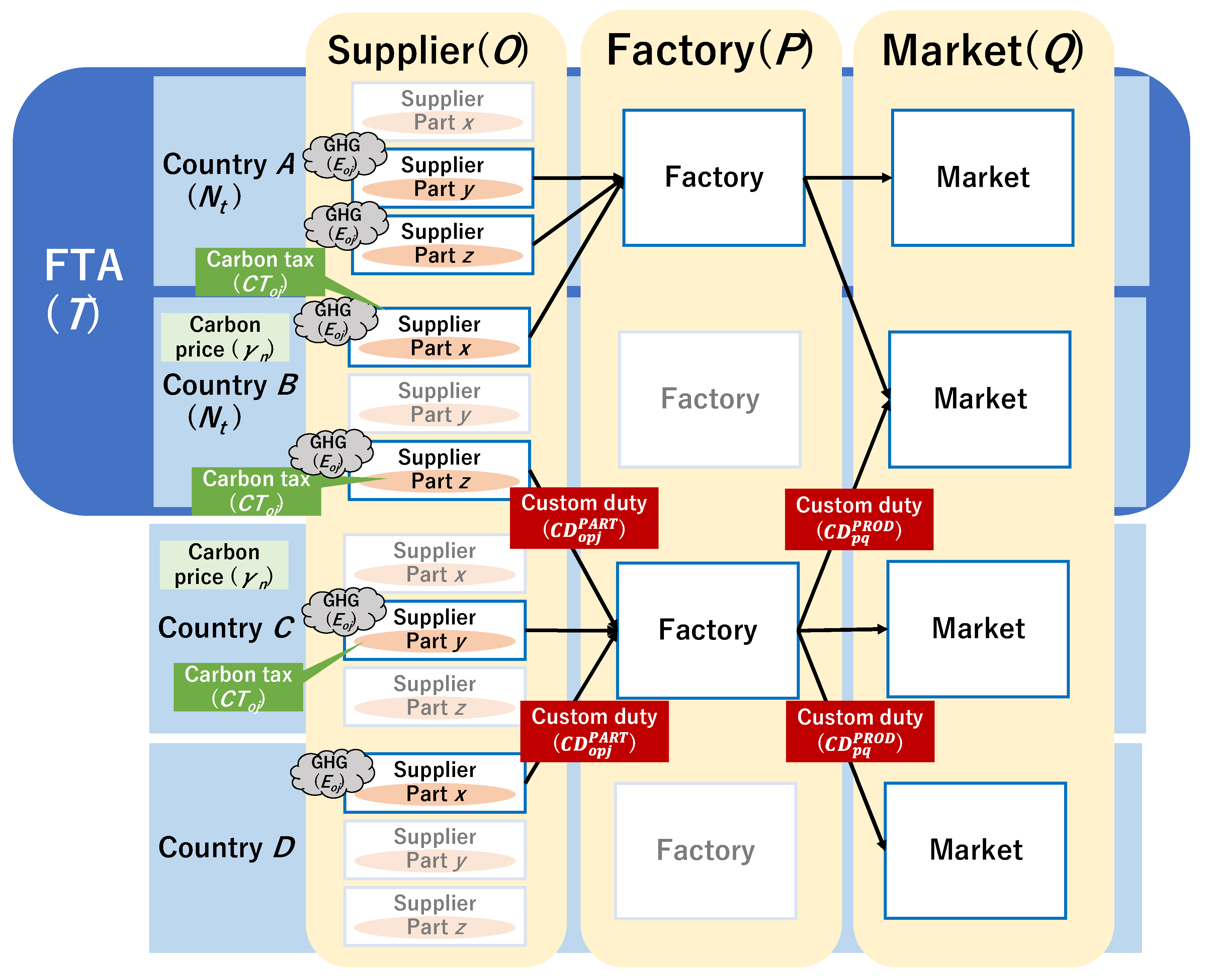
3.1. Overview of Global Supply Chain with FTAs under Different Carbon Taxes and Tariffs in Multiple Countries

The proposed supply chain network consists of suppliers, factories, and markets in multiple countries as shown in Figure 1, which shows a global supply chain network incorporating carbon taxes and FTAs. A market in this study is defined as a city where a certain volume of demand for an assembly product is expected. Figure 1 illustrates an overview of the proposed mathematical model to determine suppliers, factories, and the number of transporting parts and products so as to meet all demands in markets. The black arrows among suppliers, factories and markets indicate the transportations of parts or products between them. These arrows are determined by using the mathematical model. In the model, markets are predetermined, while suppliers and factories are determined from candidates set in advance using the mathematical model.

As shown in Figure 1, parts are procured and delivered from suppliers and assembled at factories. The assembled products are transported to each market. The suppliers and factories are selected to minimize the total cost, including procurement costs, transportation costs, manufacturing costs, fixed opening factory costs, fixed opening route between a factory and market costs, and carbon taxes and tariffs. Fixed costs for opening a route means constant indirect costs. These are for opening offices and for expatriate labor costs needed for transportation and trading of products from factories to markets.

Each country sets different carbon tax prices and tariffs. Moreover, FTAs are considered in the proposed model. In Figure 1, FTAs exist between countries A and B. Tariffs are then imposed for the international transportation of parts and products between countries without the FTA. For example, the international transportation of parts and products between countries B and C cause tariffs, as shown in Figure 1.

With respect to carbon taxes, only countries B and C introduced different carbon tax prices, as shown in Figure 1. The proposed model only considers GHG emissions for material production at the suppliers. Hence, the carbon taxes are imposed based on the amount of GHG emissions for material production and carbon tax prices of supplier countries. The GHG emissions in this study include not only CO₂ but also CH₄, N₂O, HFCs, PFC, and SF₆. A unit of g-CO₂eq denotes an amount of GHG that is equivalent to 1 g of CO₂ [3].

3.2. Formulation

Notations used in the mathematical model for the global supply chain network with FTAs under different carbon taxes and tariffs are listed as follows:

I. Sets
T	:	Set of tariff partnerships, t $\in$ T
N	:	Set of countries, m,n $\in$ N
$N_t$	:	Set of countries agreed to tariff partnership t, $N_t\subseteq N$
J	:	Set of parts, j $\in$ J
O	:	Set of suppliers, o $\in$ O
P	:	Set of factories, p $\in$ P
Q	:	Set of markets, q $\in$ Q
II. Decision variables
loj	:	Quantity of part j produced at supplier o [units]
kp	:	Quantity of the product manufactured at factory p [units]
vopj	:	Number of units of part j transported from supplier o to factory p [units]
vpq	:	Number of units of product transported from factory p to market q [units]
zpq	:	1, when route from factory p to market q is open 0, otherwise
up	:	1, when factory p is open 0, otherwise
III. Parameters
$T{C}_{op}^{PART}$	:	Transportation cost per unit of part from supplier o to factory p [USD]
$T{C}_{pq}^{PROD}$	:	Transportation cost per unit of product from factory p to market q [USD]
$P{C}_{oj}$	:	Procurement cost per unit of part j from supplier o [USD]
$M{C}_p$	:	Manufacturing cost per unit of product at factory p [USD]
$OR{C}_{pq}$	:	Fixed cost of opening a route between factory p and market q [USD]
$OF{C}_p$	:	Fixed cost of opening factory p
$N{P}_j$	:	Number of part j composing product [units]
$S_{oj}$	:	1, when supplier o can supply part j 0, otherwise
$CA{P}_p^{PROD}$	:	Production capacity of products at factory p [units]
Dq	:	Number of product units demanded in market q [units]
$\delta \left(h\right)$	:	Country of facility h, $h\in O\cup P\cup Q$
$C{D}_{opj}^{PART}$	:	Custom duty on the importation of a part j from supplier o to factory p [USD/unit]
$C{D}_{pq}^{PROD}$	:	Custom duty on the importation of a product from factory p to market q [USD/unit]
${\alpha }_{mnj}$	:	Custom duty rate on the importation a part j between countries m and n [%]
${\beta }_{mn}$	:	Custom duty rate on the importation a product between countries m and n [%]
$C{T}_{oj}$	:	Carbon tax of a part j procured from supplier o [USD/unit]
${\gamma }_n$	:	Carbon tax price in countries n [USD/t-CO2eq]
$E_{oj}$	:	Material-based greenhouse gas emissions produced by the manufacturing of part j at supplier o [g-CO2eq]
M	:	An extremely large number (big M)

This study formulates the global low-carbon supply chain network considering carbon tax and FTAs via integer programming [33]. The objective function of this study is to minimize total costs, including procurement costs, manufacturing costs, transportation costs, fixed costs of opening factory and routes, tariffs, carbon taxes. Component 1 in Equation (1) is procurement costs, transporting costs, and custom duties between suppliers and factories. Component 2 is manufacturing costs, transporting costs, and custom duties between factories and markets. Components 3 and 4 are fixed costs of opening routes between factories and markets, and opening factories. Component 5 is carbon taxes levying material-based GHG emissions.

$$\begin{array}{cc}{{\displaystyle \sum }}_{o\in O}{{\displaystyle \sum }}_{p\in P}{{\displaystyle \sum }}_{j\in J}(P{C}_{oj}+T{C}_{op}^{\mathrm{PART}}+C{D}_{opj}^{\mathrm{PART}})v_{opj}+& \\ {{\displaystyle \sum }}_{p\in P}{{\displaystyle \sum }}_{q\in Q}\left(M{C}_p+T{C}_{pq}^{\mathrm{PROD}}+C{D}_{pq}^{\mathrm{PRDC}}\right)v_{pq}+& \\ {{\displaystyle \sum }}_{p\in P}{{\displaystyle \sum }}_{q\in Q}OR{C}_{pq}{z}_{pq}+{{\displaystyle \sum }}_{p\in P}OF{C}_p{u}_p+{{\displaystyle \sum }}_{o\in O}{\displaystyle \sum }_{j\in J}C{T}_{oj}{l}_{oj}\to min& \end{array}$$

(1)

Constraints:

Equations (2)–(5) are constraints that all the needed parts are supplied to factories for assembly, and then, demands of all markets are satisfied without inventories of the parts and products. Equation (2) represents all the parts procured from each supplier that must be transported to factories. Equation (3) expresses a constraint that the suppliers can provide only certain parts based on their production ability and that the number of required parts at each factory is met by selected suppliers. Equation (4) presumes all manufactured parts at each factory are sent to markets. All the demand in each market must be satisfied as shown in Equation (5).

$${{\displaystyle \sum }}_{p\in P}{v}_{opj}=l_{oj} \forall o\in O, \forall j\in J$$

(2)

$${{\displaystyle \sum }}_{o\in O}{S}_{oj}{v}_{opj}=N{P}_j{k}_p \forall p\in P , \forall j\in J$$

(3)

$${{\displaystyle \sum }}_{q\in Q}{v}_{pq}=k_p \forall p\in P$$

(4)

$${{\displaystyle \sum }}_{p\in P}{v}_{pq}=D_q \forall q\in Q$$

(5)

Equation (6) ensures that products are transported via opened routes only. The manufactured number of products at each factory must be equal to or under its production capacity, as shown in Equation (7).

$$v_{pq}\le M{z}_{pq} \forall p\in P, \forall q\in Q$$

(6)

$$k_p\le CA{P}_p^{PROD}{u}_p \forall p\in P$$

(7)

Equations (8)–(11) are constraints about the custom duties with FTAs. Equation (8) defines the custom duty for each part between suppliers and factories with FTA ($C{D}_{opj}^{PART}$). The custom duty for each part is calculated based on the procurement cost ($P{C}_{oj}$) and the custom duty rate on the importation a part j between countries m and n (${\alpha }_{mnj}$), as shown in Equation (8). The $\delta \left(o\right)$ and $\delta \left(p\right)$ represent each country of a supplier and a factory, respectively. For example, in a case of a supplier in Boston and a factory in Tokyo, $\delta \left(\mathrm{Boston}\right)$ and $\delta \left(\mathrm{Tokyo}\right)$ represent the U.S. and Japan, respectively. Then, ${\alpha }_{\delta \left(\mathrm{Boston}\right)\delta \left(\mathrm{Tokyo}\right)j}$ means the custom duty rate of part j between the U.S. and Japan.

In addition to the custom duty of parts, the custom duty of products between a factory and a market is based on the manufacturing costs ($M{C}_p$) and the custom duty rate (${\beta }_{mn}$), as shown in Equation (9).

$$C{D}_{opj}^{PART}=P{C}_{oj}{\alpha }_{\delta \left(o\right)\delta \left(p\right)j} \forall o\in O,\forall p\in P, \forall j\in J$$

(8)

$$C{D}_{pq}^{PROD}=M{C}_p{\beta }_{\delta \left(p\right)\delta \left(q\right)} \forall p\in P, \forall q\in Q$$

(9)

The custom duty rate for each part (${\alpha }_{mnj}$) is set as 0 if there is any FTAs agreed between the countries m(supplier) and country n(factory) regarding a part j. Otherwise, a proper value should be set as custom duty of part j to import country m(supplier) to country n(factory). Note the custom duty of part j should be set as 0 if a supplier and a factory are in the same country. N_t in Equation (10) represents a subset of countries agreed FTA t.

Along with the custom duty rate for each part (${\alpha }_{mnj}$), the custom duty rate for each product (${\beta }_{mn}$) is set as shown in Equation (11).

$${\alpha }_{mnj}=\left\{\begin{array}{cc}0\hfill & \hfill if \exists t\in T s.t. m,n\in N_t\hfill \\ any given value\hfill & \hfill otherwise\hfill \end{array}\right. \forall m,n\in N,\forall j\in J$$

(10)

$${\beta }_{mn}=\left\{\begin{array}{cc}0\hfill & \hfill if \exists t\in T s.t. m,n\in N_t\hfill \\ any given value\hfill & \hfill otherwise\hfill \end{array}\right. \forall m,n\in N$$

(11)

Equation (12) expresses the carbon tax calculated based on material-based GHG emissions ($E_{oj}$) and carbon tax price (${\gamma }_m$). The carbon tax price (${\gamma }_m$) differs in each country in suppliers. As well as custom duty rates, the $\delta \left(o\right)$ means the county of a supplier o.

$$C{T}_{oj}=E_{oj}{\gamma }_{\delta \left(o\right)} \forall o\in O, \forall j\in J$$

(12)

Equation (13) enforces that the transported number of parts and products are not negative.

$$\begin{array}{cc}{v}_{opj, }{v}_{pq}\ge 0\hfill & \forall o\in O, \forall p\in P, \\ & \forall j\in J,\forall q\in Q\end{array}$$

(13)

4. Numerical Example

To illustrate a design example of carbon taxes and tariffs with FTAs in supply chain, a vacuum cleaner composed of 23 parts is used as an example product as well as Nakamura, Yamada, and Tan [19]. Example problems and parameters are set and detailed below.

4.1. Assumptions

• China, Malaysia, the U.S., and Japan are used to illustrate a design example. China and Japan have already introduced carbon tax. The carbon tax prices of China and Japan are 9.00 [USD/t-CO₂eq] and 2.00 [USD/t-CO₂eq], respectively [6]. Regarding FTA, the TPP Agreement is considered. Then, the tariff between Malaysia and Japan is set as 0.00 [USD];
• Each country has 13 suppliers. Four cities are chosen as factory candidates: Shanghai, Kuala Lumpur, Seattle, and Tokyo. Tokyo is selected as the market; the numbers of products demanded are set at 6000. The production capacity of products at each factory is set at 3000;
• The quality of parts and assembly products is the same even though the supplier or factory is different. In other words, only costs and GHG emissions at material production depend on the country located in suppliers and factories;
• Nakamura, Yamada, and Tan [19] indicated that part #19, the motor, accounted for over half of supply costs, so part #19 was excluded from numerical experiments.

4.2. Estimation Method and Assumptions Regarding Costs and GHG Emissions

The procurement costs and GHG emissions of each part are calculated by using the same method proposed in Yoshizaki et al. [31]. First, a material type and weight of each part are obtained from the 3D-CAD model. Next, the unit material price [USD/g] is estimated based on the census of manufactures [34] by assuming the exchange rate between yen and USD as 100 [yen] = 1 [USD]. Then, the procurement cost in each country is calculated using the “Residential Devices, Equipment, and Maintenance” comparison of price levels in various countries [35], as shown in

Table A1. Comparison of price levels among countries, with Japan set as 1 [35].

Price Level Index	Equipment Residential Devices Maintenance	The Total Domestic Production
China	0.57	0.40
Malaysia	0.52	0.35
The U.S.	0.64	0.74
Japan	1.00	1.00

in Appendix A as follows:

Procurement cost [USD] = weight [g] × material unit price [USD/g] × price level.

GHG emissions of each part in each country are estimated based on the LCI database with the Asian international I/O table listing the GHG emission intensity of Asian countries and the U.S. [36]. By inputting the calculated procurement cost of each part in each county to the LCI database, the material-based GHG emissions can be calculated.

Table 2. GHG emissions and procurement cost of parts in each country.

No.	Part Name	Required Number for a Product	Procurement Cost [USD]				GHG Emissions [g-CO2eq]
			China	Malaysia	The U.S.	Japan	China	Malaysia	The U.S.	Japan
1	Wheel of nozzle	2	0.0056	0.0051	0.0062	0.0098	39.82	17.16	7.48	7.51
2	Wheel stopper	2	0.0014	0.0012	0.0015	0.0024	9.63	4.15	1.81	1.82
3	Upper nozzle	1	0.0401	0.0365	0.0444	0.0698	283.59	122.20	53.25	53.51
4	Lower nozzle	1	0.0328	0.0299	0.0364	0.0572	232.33	100.11	43.62	43.84
5	Nozzle	1	0.0275	0.0250	0.0305	0.0478	194.31	83.73	36.49	36.67
6	Right handle	1	0.0390	0.0355	0.0432	0.0678	275.59	118.75	51.75	52.00
7	Switch	1	0.0033	0.0030	0.0037	0.0058	23.65	10.19	4.44	4.46
8	Left handle	1	0.0412	0.0375	0.0456	0.0716	291.19	125.47	54.67	54.95
9	Left body	1	0.1491	0.1359	0.1653	0.2595	1054.76	454.50	198.05	199.02
10	Right body	1	0.1432	0.1305	0.1588	0.2493	1013.13	436.56	190.23	191.17
11	Dust case cover	1	0.0554	0.0505	0.0614	0.0964	391.89	168.87	73.58	73.95
12	Mesh filter	1	0.3441	0.3136	0.3816	0.5990	2967.54	1211.26	557.95	438.22
13	Connection pipe	1	0.0581	0.0530	0.0644	0.1012	409.95	72.76	63.58	47.03
14	Dust case	1	0.2661	0.2425	0.2951	0.4632	1882.72	811.27	353.51	355.25
15	Exhaust tube	1	0.0230	0.0210	0.0255	0.0401	162.99	70.23	30.60	30.76
16	Upper filter	1	0.3309	0.3015	0.3669	0.5759	2853.34	1164.65	536.47	421.36
17	Lower filter	1	0.0234	0.0213	0.0259	0.0406	165.19	71.18	31.02	31.17
18	Protection cap	1	0.0251	0.0229	0.0278	0.0437	177.60	76.53	33.35	33.51
20	Rubber of outer flame of fan	1	0.0319	0.0291	0.0354	0.0556	332.83	125.15	65.88	55.96
21	Outer flame of fan	1	0.0679	0.0619	0.0753	0.1182	478.96	85.01	74.29	54.94
22	Lower fan	1	0.0120	0.0109	0.0133	0.0209	84.93	36.60	15.95	16.03
23	Fan	1	0.0765	0.0697	0.0848	0.1332	539.71	95.79	83.71	61.91

shows GHG emissions and procurement cost of parts in each country.

Our model assumes two different types of costs. One type of costs depends on the types of part and procured country, namely, procurement costs, listed in Table 2. The other depends on facilities such as the transportation costs, fixed costs of opening a factory, and fixed cost of an opening route between a factory and a market, as shown in

Table 3. Costs and production capacities at each factory.

Factory	Manufacturing Cost [USD]	Opening Factory Cost [USD]	Production Capacity [unit]	Transportation Cost [USD] (to Tokyo)	Opening Route Cost [USD] (to Tokyo)
Shanghai	2.54	726	3000	0.1760	1566
Kuala Lumpur	2.23	638	3000	0.5328	1532
Seattle	4.67	1338	3000	0.7700	1800
Tokyo	6.29	1800	3000	0.0001	600

. In numerical experiments in the paper, only Tokyo is set as a market. Then, transportation costs and fixed costs of opening routes between factories and markets can be determined by only locations of factories, as well as manufacturing costs, production capacity, and fixed costs of opening a factory. The detailed assumptions and calculated methods costs are shown in Table 3 as follows:

• Vacuum cleaner production costs use vacuum cleaner production costs in Japan found in Urata et al. [37]. The production cost is estimated using the Assembly Reliability Estimation Method, which is a method and software developed by Hitachi Ltd. [38,39]. The production cost in other countries is taken from the same documentation used for part supply costs, which is used to give a ratio for the gross domestic product for each country (Table A1) [35];
• The opening factory and opening route costs in each country are determined based on the gross domestic product [35] as well as the production cost;
• Transportation cost is estimated based on the direct distances between cities.

All numerical experiments are conducted based on the data described in Table 2 and Table 3 and

Table A2. Transportation costs between suppliers and factories.

Supplier	Factory
	Shanghai	Kuala Lumpur	Seattle	Tokyo
Guangzhou	0.0121	0.0255	0.1273	0.0291
Chongqing	0.0144	0.0299	0.1280	0.0317
Nanjing	0.0027	0.0368	0.1279	0.0197
Harbin	0.0168	0.0533	0.1299	0.0158
Xian	0.0122	0.0355	0.1294	0.0280
Chengdu	0.0166	0.0306	0.1297	0.0335
Changchun	0.0144	0.0509	0.1255	0.0152
Dalian	0.0086	0.0447	0.1239	0.0164
Hangzhou	0.0017	0.0359	0.1206	0.0192
Jinan	0.0072	0.0405	0.0339	0.0203
Qingdao	0.0055	0.0414	0.1165	0.0174
Suzhou	0.0008	0.0371	0.1238	0.0184
Fuzhou	0.0061	0.0317	0.1280	0.0222
Alor Setar	0.0356	0.0036	0.0351	0.0519
Penang	0.0363	0.0027	0.0112	0.0525
Kuantan	0.0359	0.0020	0.0312	0.0515
Malacca	0.0381	0.0012	0.0282	0.0536
Kuala Lumpur	0.0375	0.0000	0.0327	0.0533
Johor Bahru	0.0380	0.0030	0.0401	0.0532
Kuching	0.0351	0.0098	0.0343	0.0486
Sibu	0.0337	0.0113	0.0155	0.0470
Miri	0.0309	0.0137	0.0307	0.0437
Kota Kinabalu	0.0287	0.0163	0.0339	0.0409
Sandakan	0.0285	0.0184	0.0372	0.0399
Ipoh	0.0365	0.0018	0.0277	0.0525
Penang	0.0363	0.0027	0.0163	0.0525
Atlanta	0.1230	0.1586	0.0351	0.1103
San Jose	0.0995	0.1366	0.0112	0.0833
Detroit	0.1146	0.1494	0.0312	0.1012
Chicago	0.1136	0.1492	0.0282	0.1134
Cleveland	0.1158	0.1504	0.0327	0.1045
Boston	0.1173	0.1490	0.0401	0.1079
Pittsburgh	0.1174	0.1517	0.0343	0.1063
Los Angeles	0.1043	0.1414	0.0155	0.0881
Houston	0.1220	0.1593	0.0307	0.1073
New Orleans	0.1244	0.1613	0.0339	0.1105
Washington D.C.	0.1198	0.1534	0.0372	0.1090
Saint Louis	0.1158	0.1521	0.0277	0.1045
Denver	0.1078	0.1452	0.0163	0.0933
Fukuoka	0.0088	0.0451	0.1039	0.0088
Hiroshima	0.0109	0.0472	0.1014	0.0068
Yokohama	0.0175	0.0531	0.0927	0.0003
Osaka	0.0136	0.0495	0.0767	0.0040
Nagoya	0.0150	0.0509	0.0954	0.0026
Sapporo	0.0219	0.0592	0.1017	0.0083
Kumamoto	0.0089	0.0448	0.0787	0.0089
Kobe	0.0134	0.0493	0.0849	0.0042
Shizuoka	0.0163	0.0518	0.0934	0.0014
Kyoto	0.0140	0.0499	0.0894	0.0036
Sendai	0.0193	0.0558	0.0882	0.0031
Niigata	0.0177	0.0542	0.0924	0.0025
Wakayama	0.0132	0.0490	0.0977	0.0044

in Appendix A. The optimization software Nuorium Optimizer [40] is used on an Intel^®Core™i5-9400 CPU @ 2.90 GHz PC with Windows 10 Pro installed.

5. Results and Discussion

FTAs can absorb additional procurement costs owing to introducing carbon taxes by exempting customs duty. Hence, FTAs can bring a positive effect in terms of cost reduction in constructing global supply chain with carbon tax. FTAs may, however, cause a switch to a supplier with a lower carbon tax price. This economical advantage of no tariff by FTAs would provoke this phenomenon, known as carbon leakage. It occurs when the different carbon tax prices are introduced in countries and indicates increased amounts of GHG emissions in the global supply chain. Therefore, FTAs can also bring this negative effect of carbon leakage.

Manufacturers have been required to reduce GHG emissions in current supply chains. Efforts to avoid carbon leakage and reduce GHG emissions globally might unintended setbacks due to situations and conditions of FTAs and should be examined by answering RQ1. Manufactures would then need practical implications to answer RQ2, to examine cost reduction and carbon leakage by FTAs in the global low-carbon supply chain thorough numerical experiments. Section 5.1 compares the total costs and GHG emissions in the global low-carbon supply chain with and without TPP. Sensitivity analysis of carbon tax prices to identify trends or conditions for the construction of global low-carbon supply chain economically is discussed in Section 5.2, and Section 5.3 observes cost breakdowns and networks of constructed supply chain with different total costs and GHG emissions.

5.1. With vs. without FTAs for Economic Benefit and Carbon Leakage in Supply Chain

As described in Section 4, China, Malaysia, the U.S., and Japan are used as suppliers, factories, and markets. Only TPP is considered as the FTA, and then, tariff exemption is adopted for the transportation of parts and products between Malaysia and Japan. Carbon tax is introduced in China and Japan as 9 [USD/t-CO₂eq] and 2 [USD/t-CO₂eq], respectively.

First, the effects of TPP and carbon tax are examined in the design examples, in four cases with and without TPP and carbon taxes as shown in

Table 4. Total costs and GHG emissions with vs. without TPP and carbon taxes.

		Carbon Tax
		with	without
TPP	With	33,490 [USD]	33,116 [USD]
		5.81 × 107 [g-CO2eq]	5.81 × 107 [g-CO2eq]
	Without	34,159 [USD]	33,784 [USD]
		5.81 × 107 [g-CO2eq]	5.81 × 107 [g-CO2eq]

, which shows the total costs and GHG emissions in the four cases. Even though Chinese and Japanese carbon tax prices are set to simulate real situations in two out of the four cases, GHG emissions in all cases were the same. Thus, currently introduced carbon tax prices in China and Japan were not effective in the design examples. In contrast to the GHG emissions, the total costs with TPP are different and lower than ones without TPP.

Previous findings show that despite increasing carbon taxes in the past, most of the carbon tax prices in each country remains sufficiently low to drive the transformative change needed for reaching the 1.5 °C target [6]. The carbon price corridor to reach the target is estimated as 50–250 [USD/tCO₂-eq] [6]. The carbon tax prices in China and Japan would be increased and ones in Malaysia and the U.S. would be introduced. The cases of increase in Chinese and Malaysian carbon tax prices were examined to determine whether FTAs could bring positive or negative effects such as cost reduction by the elimination of tariff or carbon leakage by different carbon taxes.

In the numerical experiments, the Chinese carbon tax price was changed to 9, 90, 180, and 270 [USD/t-CO₂eq]. The Malaysian carbon tax price was also changed to 0, 100, 500, and 2000 [USD/t-CO₂eq]. The carbon tax prices of Japan and the U.S. were steady and set as 2 and 0 [USD/t-CO₂eq], respectively. Regarding tariff, the custom duties of parts and products were set at 10% in international transportation between the exception of Malaysia and Japan. In cases without TPP in the numerical experiments, the custom duty between Malaysia and Japan was also set as 10%. The results of experiments with and without TPP using these carbon tax prices are shown in Figure 2.

Figure 2 shows the differences in GHG emission and total cost in supply chain with TPP against ones without TPP. The solid bars in Figure 2 refer to the differences in GHG emissions. By contrast, the slashed bars in Figure 2 refer to the differences in total costs. For example, in the case of Chinese and Malaysian carbon tax prices set as 180 and 2000 [USD/t-CO₂eq], respectively, the GHG emission and total cost with TPP were lower by 2.61% and 2.33%, respectively, compared with ones without TPP.

Owing to TPP, the total costs in supply chain with TPP were 1.83% lower on average than ones without TPP, as shown in Figure 2. Comparing the selected factories in supply chain with and without TPP, the same factories in Shanghai and Kuala Lumpur were selected in all cases. Suppliers, however, were generally switched from ones in China and Malaysia to ones in the U.S. and Japan. From these findings, it was considered that the differences in the total costs between with and without TPP were due to changing tariffs and costs of procurement and parts transportation.

In terms of GHG emissions, most supply chains with and without TPP had the same GHG emissions, as shown in Figure 2. Only 4 out of 16 supply chains with TPP had lower GHG emissions compared to ones without TPP. One of the notable findings regarding GHG emissions (obtained from Figure 2) is that TPP did not cause carbon leakage in all cases.

When the GHG emissions in supply chains with TPP were lower than those without TPP, Chinese or Malaysian suppliers switched to Japanese ones. They had lower GHG emissions, but higher procurement costs than those in China or Malaysia, when providing parts. Therefore, international transportations of parts between Malaysia and Japan without tariffs could be increased economically. As a result, the GHG emissions in supply chains with TPP were lower than those without TPP. Based on these discussions, FTAs such as TPP may well contribute to GHG reduction with carbon tax, by enhancing international transportation from developed countries with lower GHG emissions compared to those of emerging countries.

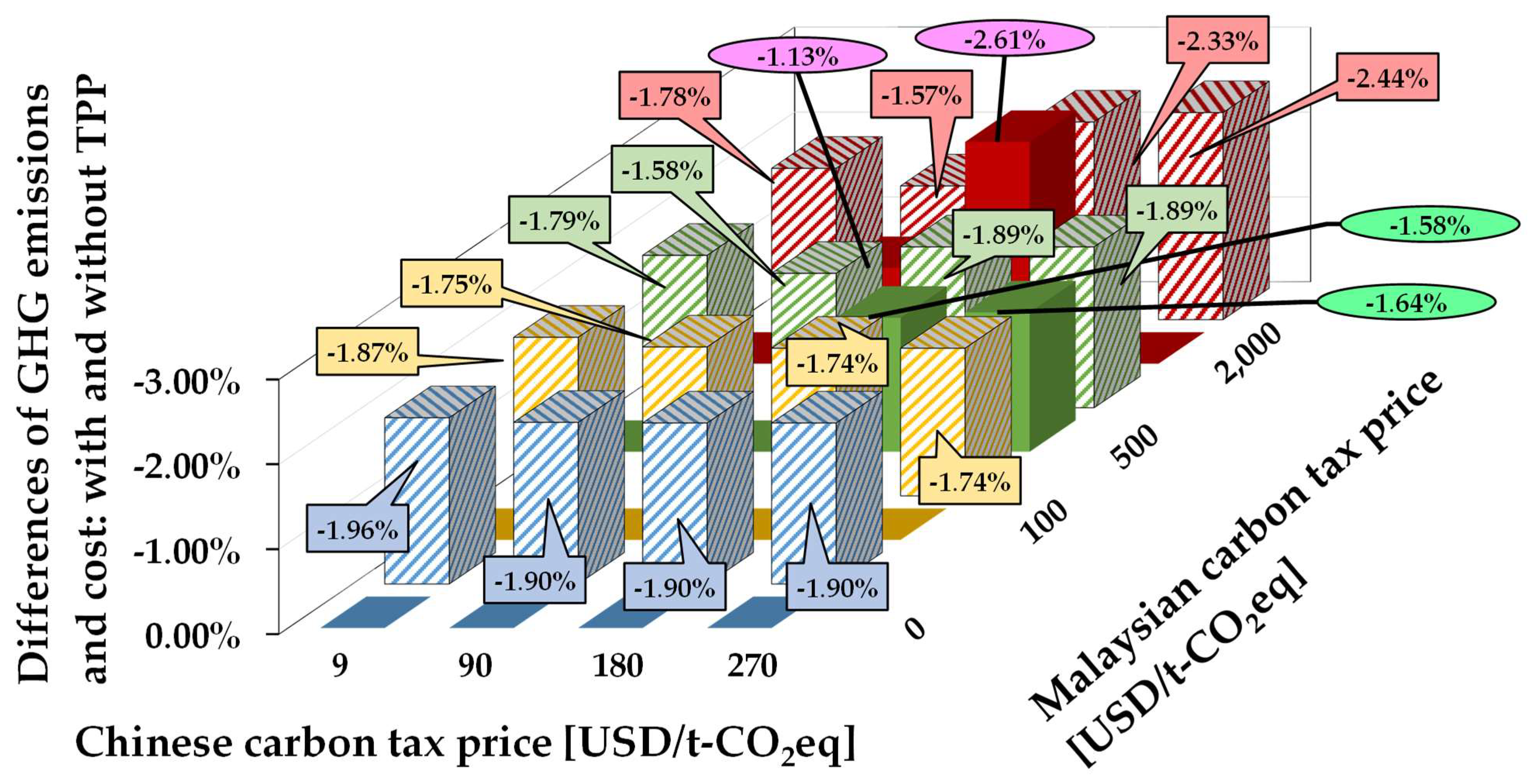
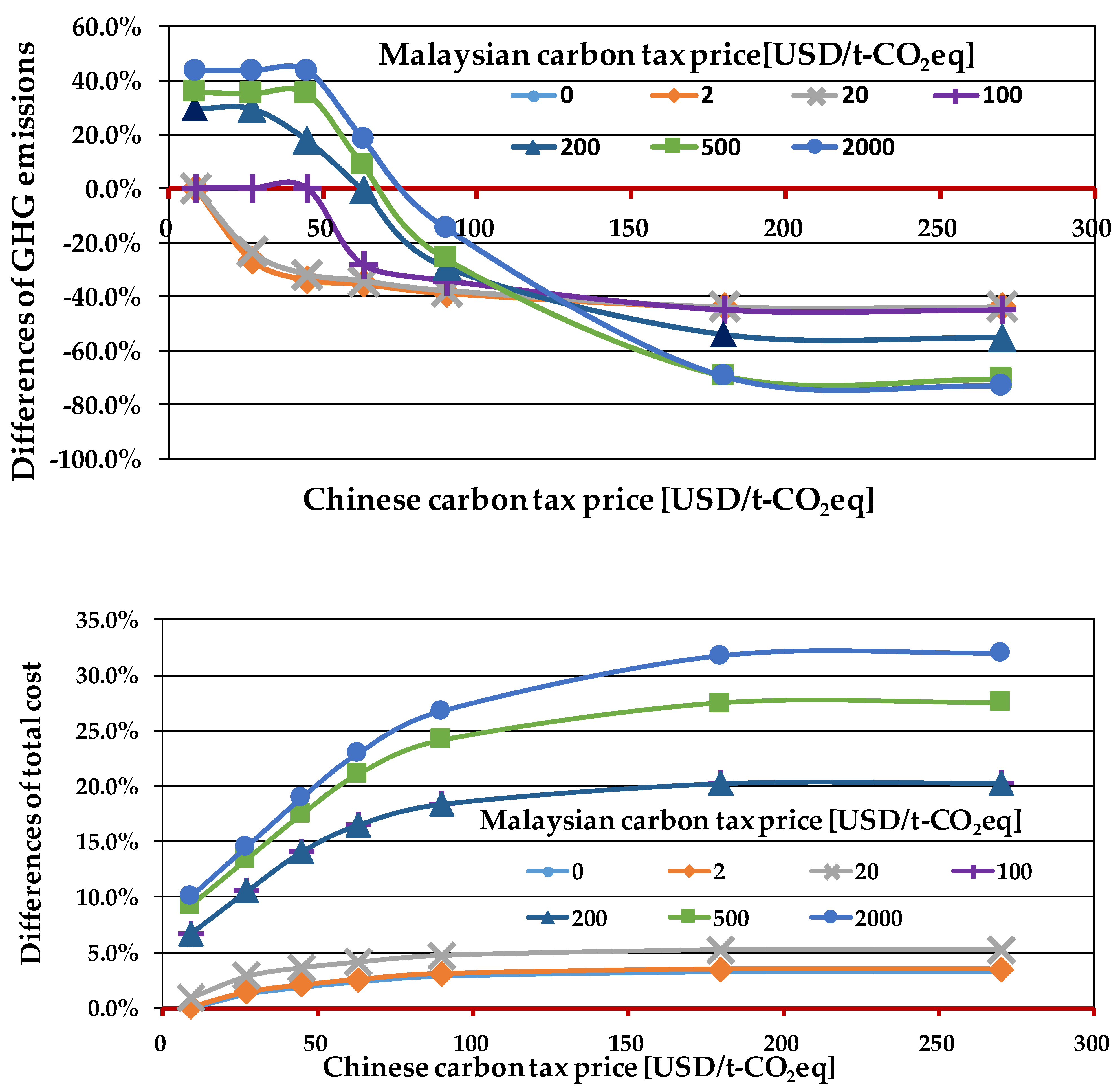
5.2. Sensitivity Analysis of Chinese and Malaysian Carbon Tax Prices with TPP

FTAs such as TPP could bring positive effects, that is, cost reduction by elimination of tariffs compared with those without FTA. The current carbon tax prices set at 9 and 2 [t-CO₂eq] in China and Japan were, however, too low to transform the global supply chain configuration into ones with lower GHG emissions. Sensitivity analysis of Chinese and Malaysian carbon tax prices was conducted to identify the proper or desirable carbon tax prices to reduce GHG emissions in the whole supply chain.

At the sensitivity analysis, Chinese and Malaysian carbon tax prices were changed, while Japanese and the U.S. were steady and set at 2 and 0 [USD/t-CO₂eq], respectively. Chine carbon tax prices was changed to 9, 27, 45, 63, 90, 180, 270 [USD/t-CO₂eq]. Malaysian carbon tax prices were also changed to 0, 2, 20, 100, 200, 500, 2000 [USD/t-CO₂eq]. To understand the reduction in GHG emissions and increment in total costs, the GHG emissions and total costs in the constructed supply chain in current carbon taxes with TPP, that is, 5.81× 10⁷ [g-CO₂eq] and 33,490 [USD], as shown in Table 4 in Section 5.1, were set as baseline.

Figure 3 shows the differences in GHG emissions and total costs compared to the ones in the baseline in the sensitivity analysis with TPP. From the upper graph in Figure 3, three findings were observed. First, the GHG emissions decreased with increasing Chinese carbon tax. Second, Chinese carbon taxes higher than 180 [USD/t-CO₂eq] were not effective in reducing GHG emissions. This could be because GHG emissions in Chinese carbon tax prices set at 270 [USD/t-CO₂eq] were almost the same as Chinese carbon tax prices set at 180 as shown in the upper graph in Figure 3. Finally, carbon leakages occurred in 11 cases. The carbon leakages were observed at the Chinese carbon tax prices equal to or lower than 63 [USD/t-CO₂eq] and at Malaysian carbon tax prices equal to or higher than 200 [USD/t-CO₂eq]. Especially, in the cases of Malaysian carbon tax set at 2000 [USD/t-CO₂eq], the GHG emissions in other supply chains increased by 40% compared to the ones at the baseline.

In the case of Malaysian carbon tax prices equal to or higher than 500 [USD/t-CO₂eq], significant reductions in GHG emissions were achieved, by approximately 70%. Based on these findings, the Malaysian carbon tax prices may be more sensitive than Chinese ones for GHG emissions. The higher Malaysian carbon tax prices, more than 200, might have the potential to reduce GHG emissions in the supply chains significantly despite risks of carbon leakages.

The lower graph in Figure 3 shows total costs in sensitivity analysis compared to the baseline. Compared to the behaviors of GHG emissions in the upper graph in Figure 3, the behaviors of the total costs were uncomplicated and increased generally as the Chinese and Malaysian carbon prices increased. Regarding the cases with Chinese carbon tax prices set at 270, the total costs were almost the same as the cases of the Chinese carbon tax prices set at 180. This trend was observed for all the different Malaysian carbon tax prices set. Thus, in contrast to GHG emissions, total costs can be predicted from the carbon tax prices of each country, without employing the mathematical optimization models.

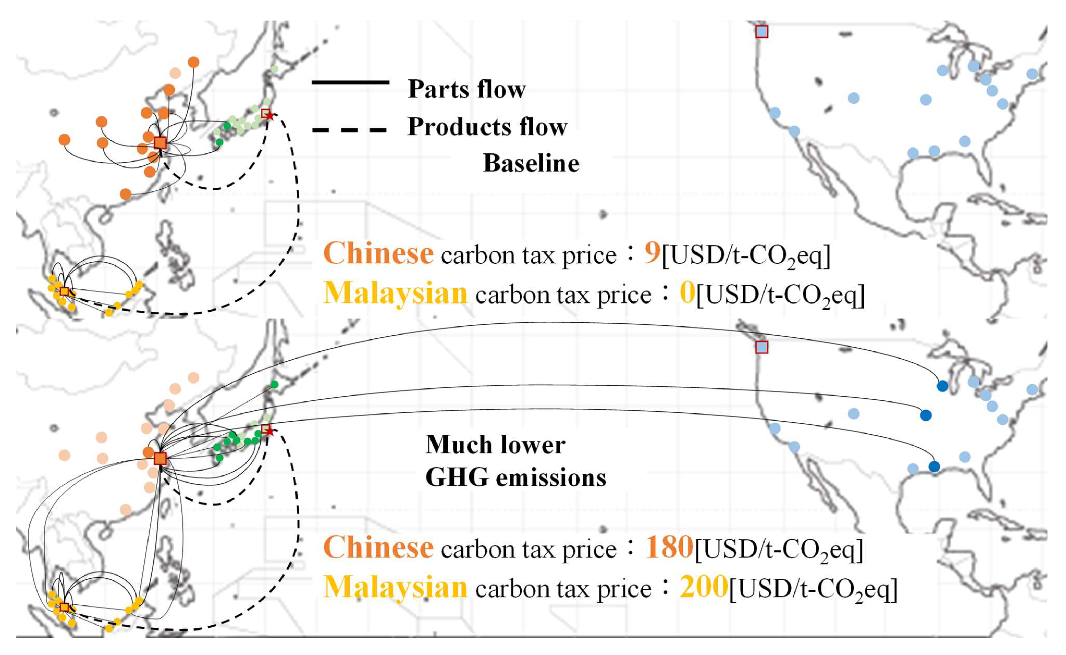
5.3. Analysis of GHG Emissions, Cost Breakdowns, and Constructed Supply Chain Network

The four featured cases are represented as four scenarios so that practical implications will be sought to reduce GHG emissions. This is to avoid carbon leakages by comparing GHG emissions, cost breakdowns, and constructed supply chain networks.

Table 5. Summary of scenarios.

Scenario	Chinese Carbon Tax [USD/t-CO2eq]	Malaysian Carbon Tax [USD/t-CO2eq]	Difference of GHG Emissions [%]	Difference of Total Costs [%]
Baseline	9	0	-	-
Little lower GHG emissions	27	0	−26.30	1.28
Much lower GHG emissions	180	200	−54.00	20.26
Carbon leakage	9	200	29.40	6.73

summarizes the four scenarios. “Baseline” indicates the current actual carbon tax prices. “Little lower GHG emissions” is the most cost-effective scenario for GHG reduction. “Much lower GHG emissions” is a scenario in which the Japanese target of reducing GHG emissions by 2030 is achieved. In “Carbon leakage”, carbon leakage occurs such that the total GHG emission in the supply chain increases. This was compared to the baseline despite introducing carbon taxes.

Table 6. Cost breakdowns and GHG emissions in each scenario.

Scenario		Baseline		Little Lower GHG Emissions		Much Lower GHG Emissions		Carbon Leakage
Procurement cost [USD]		10,360.75	30.94%	10,072.33	29.70%	11,115.34	27.60%	10,688.82	29.90%
Manufacturing cost [USD]		14,293.81	42.68%	14,293.81	42.14%	14,293.81	35.49%	14,293.81	39.99%
Transportation cost [USD]		3235.58	9.66%	3612.00	10.65%	4803.98	11.93%	3685.60	10.31%
Open route cost [USD]		3098.00	9.25%	3098.00	9.13%	3098.00	7.69%	3098.00	8.67%
Open factory cost [USD]		1363.48	4.07%	1363.48	4.02%	1363.48	3.39%	1363.48	3.81%
Custom duty [USD]		764.06	2.28%	1060.50	3.13%	1367.03	3.39%	1134.07	3.17%
Carbon tax [USD]	China	374.55	1.12%	417.59	1.23%	153.14	0.38%	638.38	1.79%
	Malaysia	0.00	0.00%	0.00	0.00%	4078.13	10.13%	843.11	2.36%
	The U.S.	0.00	0.00%	0.00	0.00%	0.00	0.00%	0.00	0.00%
	Japan	0.05	0.00%	0.05	0.00%	2.27	0.01%	0.05	0.00%
Total costs [USD]		33,490.27		33,917.76		40,275.18		35,745.31
GHG emissions [g-CO2eq]	China	4.16 × 107	71.64%	1.55 × 107	36.13%	8.51 × 105	3.18%	7.09 × 107	94.36%
	Malaysia	1.65 × 107	28.32%	2.73 × 107	63.82%	2.04 × 107	76.31%	4.22 × 106	5.61%
	The U.S.	0.00	0.00%	0.00	0.00%	4.34 × 106	16.26%	0.00	0.00%
	Japan	2.43 × 104	0.04%	2.43 × 104	0.06%	1.13 × 106	4.24%	2.43 × 104	0.03%
Total GHG emissions [g-CO2eq]		5.81 × 107		4.28 × 107		2.67 × 107		7.52 × 107

shows the cost breakdowns and GHG emissions in each scenario. The percentages of cost and GHG emissions denote the ratio against total costs and total GHG emissions, respectively. It is important for the decision makers to grasp cost breakdown and GHG emissions at each country so as to deal with cost fluctuation. This is because the tariffs and carbon tax prices would be changed largely and rapidly since they are affected by political decisions. Comparing “Baseline” and “Little lower GHG emissions,” the total costs and cost breakdowns were almost the same. One main difference between them was the Malaysian GHG emissions, as shown in Table 6. The Malaysian GHG emissions in a “Lower GHG emissions” scenario was approximately 65% higher than that in “Baseline”. For the Malaysian government, this situation would be undesirable but could become desirable if the GHG emissions could be reduced globally by switching Chinese suppliers to Malaysian ones.

In “Much lower GHG emissions”, the transportation costs and custom duty increased by 48% and 79% compared to that in “Baseline,” respectively. Figure 4 shows constructed global supply chains in “Baseline” and “Much lower GHG emissions”. The circles and squares express locations of suppliers and factories in each country. The selected suppliers and opened factories are marked with a stronger color. The contribution of Figure 4 is that the locations of selected suppliers can be understood at a glance. It also indicates one example that how a global low-carbon supply chain should be constructed for the reduction of GHG emissions. The decision makers of supply chains need to decide which suppliers should be selected and where factories should be opened to reduce GHG emissions economically by comparing costs and GHG emissions. However, the locations of suppliers and factories, cost breakdown, and GHG emissions at each country cannot be grasped from Figure 3 since they have only total GHG emissions and costs in whole supply chains.

As shown in Figure 4, the Chinese and Malaysian factories were opened at both scenarios. In contrast to the factories, the selected suppliers were different since most suppliers in China was switched to ones in Malaysia in “Much lower GHG emissions”, as shown in Figure 4. In the “Baseline” scenario, the Chinese factory procured parts from 11 Chinese and 2 Japanese suppliers. That is, most of domestic suppliers were selected at the Chinese factory in the “Baseline” scenario. On the other hand, at the Chinese factory in “Much lower GHG emissions”, one Chinese, nine Japanese, five Malaysian, and three U.S. suppliers were selected. Thus, the international transportation of parts for assembling at the Chinese factory increased, and therefore, the transportation costs and custom duty increased.

In the “Carbon leakage” scenario, Chinese GHG emissions increased but the Malaysian ones decreased compared to that in the “Baseline” scenario, as shown in Table 6. This indicates that switching Malaysian suppliers to Chinese ones caused carbon leakages. In “Carbon leakage”, the Malaysian carbon tax prices was over 20 times higher than that of China, as shown in Table 5. Actual differences in carbon tax prices of suppliers can increase by more than 20 times because higher carbon tax prices such as the ones in Sweden and Switzerland are over 130 [USD/t-CO₂-eq] but lower carbon tax prices such as the Japanese one are under 5 [USD]. The percentage of the Chinese GHG emissions against the total GHG emissions was about 94% in the “Carbon leakage” scenario. Thus, in the “Carbon leakage” scenario, the total costs could increase largely if Chinese government decided the increment in the Chinese carbon tax price.

In “Little lower GHG emissions”, “Much lower GHG emissions”, and “Carbon leakage” scenarios, the custom duty increased compared to one of the “Baseline” scenarios. Thus, the cost reduction without tariff by TPP might be small. By considering other FTAs such as the RCEP that agreed to 15 countries including China, Malaysia, and Japan, the total costs in “Little lower GHG emissions” and “Much lower GHG emissions” would be lower than those with TPP only. Furthermore, there is a possibility to prevent carbon leakage by enhancing international transportation of parts from developed countries with lower GHG emissions.

6. Discussion

This Section discuss the results shown in Section 5 in detail to answer RQs described in Section 1, and to state the practical implications.

(1)

(RQ1) Does FTA have a positive or negative effect on the economical construction of a low-carbon supply chain?

From the numerical experiments and discussions in Section 5.1, FTAs such as TPP can bring positive effects to reduce GHG emissions by enhancing international transportation from countries with lower GHG emissions. However, the effects of FTAs to reduce GHG emissions would not be strong since only 4 out of 16 cases with TPP could reduce GHG emissions compared to those without TPP, as shown in Figure 2.

One remarkable finding observed from Figure 2 was that the negative effects of FTAs to cause carbon leakage directory were not observed. Figure 2 denotes the differences in GHG emissions and total costs with TPP compared to those without TPP. Thus, the direct positive and negative effects of TPP can be seen from it. Therefore, FTAs such as TPP could have little effects to reduce GHG emissions, while it would also have a little possibility to be a main cause of carbon leakage.

(2)

(RQ2) How should manufacturers take advantages of FTAs for the construction of supply chain to reduce costs and GHG emissions simultaneously?

Manufactures should utilize FTAs for cost reduction by eliminating tariffs since, as described in preceding subsection, FTAs such as TPP could bring positive effects. In the “Little lower GHG emissions” and “Much lower GHG emissions” scenarios in Section 5.3, the international transportation increased, and then, custom duty increased. Taking account into other FTAs such as RCEP, the GHG emissions would be reduced with lower costs than those in “Little lower GHG emissions” and “Much lower GHG emissions” scenarios. As increasing the international transportation, the need of addressing the GHG emissions at transportation will increase. Note that the proposed model does not consider GHG emissions at transportations.

(3)

Effect of carbon tax prices on future logistics

Carbon tax can reduce GHG emissions in the whole supply chain since most of the cases in the sensitive analysis of carbon tax prices, in Figure 3 can reduce GHG emissions by switching suppliers only. However, it was also observed to cause carbon leakage due to much differences in carbon tax prices among countries. There are possibilities that differences in carbon price tax will be larger since The World Bank states carbon tax prices will increase globally [6]. Therefore, it is expected to collect and share GHG emissions in supply chains automatically [12] to prevent carbon leakage.

On the other hand, higher carbon tax prices would have both the potential to cause carbon leakages and reduce GHG emissions significantly. When the Malaysia carbon tax prices were equal to or over 200 [USD/t-CO2eq] with FTAs, carbon leakages occurred. These cases could, however, achieve over 50% reduction in GHG emissions compared to that of the baseline provided the Chinese carbon tax price was equal to or over 180 [USD/t-CO₂eq].

7. Conclusions and Future Studies

This study addressed the global low-carbon supply chain with FTAs under different carbon tax prices introduced in multiple countries. A mathematical model to minimize the total costs including carbon taxes and custom duty was proposed as a decision support model and then validated through numerical experiments. Sensitivity analysis of carbon tax prices was conducted to examine whether FTAs bring positive effects such as cost reduction without tariffs or negative effects such as causing carbon leakages.

From the numerical experiments, FTAs would not cause carbon leakage directly, and could reduce GHG emissions economically by eliminating tariffs. The possibilities were demonstrated to reduce total costs keeping with lower GHG emissions globally by taking other FTAs such as RCEP. Additionally, the high differences in carbon tax prices, such as over 20 times among countries, have the risks of carbon leakage.

Future studies should consider other carbon policies such as carbon cap-and-trade. To prevent global warming, carbon neutrality [42] (which meets the actual GHG emissions and absorption of GHG volumes by forests, etc.) should be globally achieved by in the early 2050s for a 1.5 °C (2.7 °F) target [43]. Moreover, the reverse supply chain [44] should be considered in future studies because re-useable parts and material recycling can save additional GHG emissions at the virgin material production stage [45,46].

References

1. Ravindran, A.R.; Warsing, D.P., Jr. Supply Chain Engineering: Models and Applications; CRC Press: Boca Raton, FL, USA, 2013. [Google Scholar]
2. Joshi, S. A review on sustainable supply chain network design: Dimensions, paradigms, concepts, framework and future directions. Sustain. Oper. Comput. 2022, 3, 136–148. [Google Scholar] [CrossRef]
3. Kokubu, K.; Itsubo, N.; Nakajima, M.; Yamada, T. Low-Carbon Supply Chain Management; Chuokeizai-sha, Holdings, Inc.: Tokyo, Japan, 2015. (In Japanese) [Google Scholar]
4. Waltho, C.; Elhedhli, S.; Gzara, F. Green supply chain network design: A review focused on policy adoption and emission quantification. Int. J. Prod. Econ. 2019, 208, 305–318. [Google Scholar] [CrossRef]
5. Kondo, R.; Kinoshita, Y.; Yamada, T. Green procurement decisions with carbon leakage by global suppliers and order quantities under different carbon tax. Sustainability 2019, 11, 3710. [Google Scholar] [CrossRef]
6. The World Bank. State and Trends of Carbon Pricing 2022. Available online: https://openknowledge.worldbank.org/handle/10986/37455 (accessed on 31 December 2022).
7. Martin, R.; Muûls, M.; de Preux, L.B.; Wagner, U.J. On the empirical content of carbon leakage criteria in the EU Emissions Trading Scheme. Ecol. Econ. 2014, 105, 78–88. [Google Scholar] [CrossRef]
8. Onat, N.C.; Kucukvar, M. Carbon footprint of construction industry: A global review and supply chain analysis. Renew. Sustain. Energy Rev. 2020, 124, 78–88. [Google Scholar] [CrossRef]
9. JETRO. Jetro Trade Handbook 2017; Japan External Trade Organization: Tokyo, Japan, 2017. (In Japanese)
10. Ministry of Economy, Trade and Industry. Trans Pacific Partnership (TPP). Available online: https://www.meti.go.jp/policy/external_economy/trade/tpp/index.html (accessed on 2 May 2023). (In Japanese).
11. Tian, K.; Zhang, Y.; Li, Y.; Ming, X.; Jiang, S.; Duan, H.; Yang, C.; Wang, S. Regional trade agreement burdens global carbon emissions mitigation. Nat. Commun. 2022, 13, 408. [Google Scholar] [CrossRef]
12. Nitsche, B. Exploring the Potentials of automation in logistics and supply chain management: Paving the way for autonomous supply chains. Logistics 2021, 5, 51. [Google Scholar] [CrossRef]
13. Nitsche, B. Decrypting the Belt and Road Initiative: Barriers and development paths for global logistics networks. Sustainability 2020, 12, 9110. [Google Scholar] [CrossRef]
14. Cohen, M.A.; Fisher, M.; Jaikumar, R. International Manufacturing and Distribution Networks: A Normative Model Framework. In Managing International Manufacturing; Ferdows, K., Ed.; Elsevier: Amsterdam, The Netherlands, 1989; pp. 67–93. [Google Scholar]
15. Vidal, C.J.; Goetschalckx, M.A. A Global supply chain model with transfer pricing and transportation cost allocation. Eur. J. Oper. Res. 2001, 129, 134–158. [Google Scholar] [CrossRef]
16. Tsiakis, P.; Papageorgiou, L.G. Optimal production allocation and distribution supply chain networks. Int. J. Prod. Econ. 2008, 111, 468–483. [Google Scholar] [CrossRef]
17. Amin, S.H.; Baki, F. A facility location model for global closed-loop supply chain network design. Appl. Math. Modell. 2017, 41, 316–330. [Google Scholar] [CrossRef]
18. Nakamura, K.; Ijuin, H.; Yamada, T.; Ishigaki, A.; Inoue, M. Design and analysis of global supply chain network with trans-pacific partnership under fluctuating material prices. Int. J. Smart Comput. Artif. Intell. 2019, 3, 17–34. [Google Scholar] [CrossRef]
19. Nakamura, K.; Yamada, T.; Tan, K.H. The impact of brexit on designing a material-based global supply chain network for Asian manufacturers. Manag. Environ. Qual. Int. J. 2019, 30, 980–1000. [Google Scholar] [CrossRef]
20. Kuo, T.C.; Lee, Y. Using Pareto optimization to support supply chain network design within environmental footprint impact assessment. Sustainability 2019, 11, 452. [Google Scholar] [CrossRef]
21. Aldoukhi, M.A.; Gupta, S.M. A robust closed loop supply chain network design under different carbon emission policies. Pamukkale Univ. J. Eng. Sci. 2019, 25, 1020–1032. [Google Scholar] [CrossRef]
22. Liu, M.; Li, Z.; Anwar, S.; Zhang, Y. Supply chain carbon emission reductions and coordination when consumers have a strong preference for low-carbon products. Environ. Sci. Pollut. Res. 2021, 28, 19969–19983. [Google Scholar] [CrossRef]
23. Shen, L.; Wang, X.; Liu, Q.; Wang, Y.; Lv, L.; Tang, R. Carbon trading mechanism, low-carbon e-commerce supply chain and sustainable development. Mathematics 2021, 9, 1717. [Google Scholar] [CrossRef]
24. Fahimnia, B.; Sarkis, J.; Choudhary, A.; Eshragh, A. Tactical supply chain planning under a carbon tax policy scheme: A case study. Int. J. Prod. Econ. 2015, 164, 206–215. [Google Scholar] [CrossRef]
25. Zakeri, A.; Dehghanian, F.; Fahimnia, B.; Sarkis, J. Carbon pricing versus emissions trading: A supply chain planning perspective. Int. J. Prod. Econ. 2015, 164, 197–205. [Google Scholar] [CrossRef]
26. Abdallah, T.; Farhat, A.; Diabat, A.; Kennedy, S. Green supply chain with carbon trading and environmental sourcing: Formulation and life cycle assessment. Appl. Math. Modell. 2012, 36, 4271–4285. [Google Scholar] [CrossRef]
27. Sherafati, M.; Bashiri, M.; Tavakkoli-Moghaddam, R.; Pishvaee, M.S. Achieving sustainable development of supply chain by incorporating various carbon regulatory mechanisms. Transp. Res. Part D Transp. Environ. 2020, 81, 102253. [Google Scholar] [CrossRef]
28. Alkhayyal, B.A.; Gupta, S.M. The impact of carbon emissions policies on reverse supply chain network design. Doğuş Üniversitesi Derg. 2018, 19, 99–111. [Google Scholar] [CrossRef]
29. Urata, T.; Yamada, T.; Itsubo, N.; Inoue, M. Global supply chain network design and Asian analysis with material-based carbon emissions and tax. Comput. Ind. Eng. 2017, 113, 779–792. [Google Scholar] [CrossRef]
30. SimaPro, About SimaPro. Available online: https://simapro.com/about/ (accessed on 28 April 2023).
31. Yoshizaki, Y.; Yamada, T.; Itsubo, N.; Inoue, M. Material based low-carbon and economic supplier selection with estimation of GHG emissions and affordable cost increment for parts production among multiple Asian countries. J. Jpn. Ind. Manag. Assoc. 2016, 66, 435–442. [Google Scholar]
32. Ministry of the Environment. “Supply-Chain Emissions” in Japan. Available online: https://www.env.go.jp/earth/ondanka/supply_chain/gvc/en/files/supply_chain_en.pdf (accessed on 23 April 2023).
33. Hiller, F.S.; Lieberman, G.J. Introduction to Operations Research, 8th ed.; McGraw-Hill Higher Education: New York, NY, USA, 2005. [Google Scholar]
34. Ministry of Economy, Trade and Industry. Census of Manufacture. Available online: http://www.meti.go.jp/statistics/tyo/kougyo/result-2/h17/kakuho/hinmoku/index.html (accessed on 2 May 2023). (In Japanese).
35. Ministry of Internal Affairs and Communication. New International Comparisons of GDP and Consumption Based on Purchasing Power Parities for the Year 2014 Gross Domestic Product at Current PPPs and Current Exchanges Rates. Available online: https://www.soumu.go.jp/toukei_toukatsu/index/kokusai/icp.html (accessed on 2 May 2023). (In Japanese).
36. Horiguchi, K.; Tsujimoto, M.; Yamaguchi, H.; Itsubo, N. Development of greenhouse gases emission intensity in eastern Asia using Asian international input-output table. In Proceedings of the 7th Meeting of the Institute of Life Cycle Assessment, Chiba, Japan, 7–9 March 2012; pp. 236–239. (In Japanese). [Google Scholar]
37. Urata, T.; Yamada, T.; Igarashi, K.; Inoue, M.; Kinoshita, Y. Case study on comparison analysis of assembly/disassembly operations and systems between product and production designs. J. Soc. Plant Eng. Jpn. 2015, 27, 82–91. (In Japanese) [Google Scholar]
38. Suzuki, T.; Arimoto, S.; Ueno, Y.; Kawasaki, H.; Matsumoto, Y.; Tanase, H. Study of the assembling reliability. In Evaluation 13th Design Engineering, System Section Lecture; Japan Society of Mechanical Engineers: Kanazawa, Japan, 2003; pp. 262–265. (In Japanese) [Google Scholar]
39. Ueno, Y.; Tanase, H.; Suzuki, T.; Arimoto, S.; Kawsasaki, H.; Matsumoto, Y. Study of the Assembling Reliability Evaluation (Application to the Plumbing Work of the Heavy Industrial Machine Product). In The 14th Design Engineering, System Section Lecture; Japan Society of Mechanical Engineers: Fukuoka, Japan, 2014; pp. 168–171. (In Japanese) [Google Scholar]
40. NTT Data Mathematical Systems Corporation. Nuorium Optimizer. Available online: http://www.msi.co.jp/nuopt/ (accessed on 31 December 2022). (In Japanese).
41. 3kaku-K, Blank Map Specialty Store. Available online: https://www.freemap.jp/ (accessed on 31 December 2022). (In Japanese).
42. European Parliament. What Is Carbon Neutrality and How Can It Be Achieved by 2050? Available online: https://www.europarl.europa.eu/news/en/headlines/society/20190926STO62270/what-is-carbon-neutrality-and-how-can-it-be-achieved-by-2050 (accessed on 2 May 2023).
43. The Intergovernmental Panel on Climate Change (IPCC). The Evidence Is Clear: The Time for Action Is Now. We Can Halve Emissions by 2030. Available online: https://www.ipcc.ch/2022/04/04/ipcc-ar6-wgiii-pressrelease/ (accessed on 2 May 2023).
44. Ijuin, H.; Kinoshita, Y.; Yamada, T.; Ishigaki, A. Designing individual material recovery in reverse supply chain using linear physical programming at the digital transformation edge. J. Jpn. Ind. Manag. Assoc. 2022, 72, 259–271. [Google Scholar] [CrossRef]
45. Kinoshita, Y.; Yamada, T.; Gupta, S.M.; Ishigaki, A.; Inoue, M. Analysis of cost effectiveness by material type for CO2 saving and recycling rates in disassembly parts selection using goal programming. J. Adv. Mech. Des. Syst. Manuf. 2018, 12, 1–18. [Google Scholar] [CrossRef]
46. Hasegawa, S.; Kinoshita, Y.; Yamada, T.; Bracke, S. Life cycle option selection of disassembly parts for material-based CO2 saving rate and recovery cost: Analysis of different market value and labor cost for reused parts in German and Japanese cases. Int. J. Prod. Econ. 2019, 213, 229–242. [Google Scholar] [CrossRef]
Figure 1. Global supply chain network incorporating carbon taxes and FTAs.
Logistics 07 00032 g001
Figure 2. Differences in GHG emissions and cost in supply chain with and without TPP.
Logistics 07 00032 g002
Figure 3. GHG emissions (upper) and total costs (lower) in sensitivity analysis compared to baseline.
Logistics 07 00032 g003
Figure 4. Constructed global supply chains in the “Baseline” and “Much lower GHG emissions” scenarios. Map source: 3kaku-K [41].
Logistics 07 00032 g004