A Novel Green Logistics Technique for Planning Merchandise Deliveries: A Case Study

Abstract

Background: The health crisis due to COVID-19 has changed the habits of social coexistence and therefore has had a significant impact on several economic sectors, including logistics. Nowadays, this sector faces one of the most difficult challenges in history and hence has carried out innovative strategies to adjust to the new normal and guarantee the permanence of the supply chain. In this paper, a novel green logistics technique for planning merchandise deliveries is introduced herein. Methods: This technique is based on a modified version of the Resistive Grid Path Planning Methodology (RGPPM) to establish a path through georeferential locations for delivering merchandise to customers. To do this, multi-connected resistive grids are based at customer locations for searching the path connecting the positions through electronic circuit analysis techniques. Results: Experimental results reveal that the proposed method can find a minimum spanning tree that connects all hand-over points by a continuous path. This finding has represented a reduction of around 45% in the length of the path with respect to the longest path. Conclusions: Finally, this technique is capable of addressing different optimization strategies, locating a merchandise distribution center and exploring environmental standards to reduce fuel consumption.

1. Introduction

At the end of 2019, the outbreak of coronavirus disease (COVID-19) emerged in China. SARS-COV-2 virus spreading has significantly disrupted global production chains causing serious disturbances in the supply chain [1]. According to International Labor Organization (ILO), the health security measures such as social distancing and the stoppage of non-essential activities have affected around 2.7 billion workers; i.e., 81% of the world’s workforce. Therefore, it is estimated that 1.25 billion workers in the world remain at risk of losing their job because they belong to the sectors where the impact of COVID-19 has been most significant, particularly in accommodation services, the manufacturing industry, commerce, and food services.

Health contingency has devastated the world of work causing immense human suffering and exposing the extreme vulnerability of millions of people and companies. According to the report [2] of an Intergovernmental Science-Policy Platform on Biodiversity and Ecosystem Services (IPBES) workshop on diversity and pandemics, the pandemics in the near future will emerge more frequently, and they will have a greater impact on the global economy. Therefore, it is important that the most vulnerable companies such as: micro, small, and medium-sized companies explore strategies and technological techniques that help them to go through these pandemic events. This paper explores an emerging technique in order to deliver merchandise during confinement events.

Food deliveries have increased dramatically in many countries since 2020 due to mobility restrictions and restaurant closures as a result of the coronavirus pandemic event [3]. Companies in the online food distribution industry estimate that many of their first-time online shoppers have experienced the benefits and intend not to revert to their pre-crisis habits [4]. This opens up the possibility for exponential growth in activities related to the distribution and transportation of meals and food. However, the movement of vehicles to customers in order to deliver merchandise generates a significant amount of CO₂ emissions that affect the quality of life of citizens and the climate [5,6]. Therefore, it is important to establish a green strategy for the logistics and distribution of merchandise [7].

Logistics [8,9] is a fundamental stage in the global economy and therefore it must be strategically transformed with regard to carbon emissions. Green logistics [10,11] explore the measurement and minimization of environmental impact during logistics activities.

Green strategies [12,13] are a series of actions aimed at the interrelation between social awareness and business problems. Companies with large volumes of transport and distribution pursue green climate protection strategies to avoid CO₂ emissions. On the other hand, for the transport industry, green strategies mean not only a reduction in CO₂ emissions but also significant economic savings due to optimization methods for planning the distribution of merchandise, for example, path planning is a critical point for optimizing the transfer of merchandise because, depending on how well the green strategy is carried out, it it is possible to reduce from 10% to 30% of the distance in kilometers and, consequently, the carbon emissions into the atmosphere and fuel consumption, which represents social and economic benefits. This paper proposes a green strategy focused on path planning for delivering merchandise with the purpose of reducing CO₂ emissions and therefore cause social and economic benefits.

Lecheria y Quesos Artesanales “Los Ángeles” is a Mexican startup that markets products derived from milk. Since the beginning of 2020, the enterprise has maintained the distribution of merchandise in four principal cities: Puebla, Xalapa, Veracruz, and Boca del Rio. As a result of the health emergency and the restrictions for opening a commercial space in order to serve customers, the startup has been forced to migrate towards a strategy for delivering merchandise at private homes. This paper exposes the experimental results of having carried out a new green technique for planning merchandise deliveries using the database of customers coming from the business Lecheria y Quesos Artesanales “Los Ángeles”.

Due to the increase in e-commerce and the high demand in the delivery of merchandise to the particular locations of customers, the vast majority of businesses and companies need to carry out innovative strategies to remove problems in last mile logistics [14]. According to the literature [15], there is a famous problem that has been explored in practical real-life situations for the purpose of minimizing last mile costs, it is known as the traveling salesman problem. This problem has been considered a fundamental piece for vehicle routing in the logistics area [16]. Basically, it is possible to relate this problem to the need for customers to be visited with the intention of delivering merchandise or packages starting from a base position on the map. This paper explores a novel technique for delivering merchandise in the last mile logistics.

Although the best technique for this type of problem is unknown, the following research proposes an original strategy related to the behavior of the physical phenomenon of electric current, from the perspective of circuit theory, in order to deliver merchandise in the last mile. Moreover, the exploration of this approach opens the possibility of laying the foundations to face computational problems as the number of customers increases.

The manuscript is organized as follows: Section 2 introduces the proposed RGPPM algorithm for planning merchandise deliveries. In Section 3, the experimental results are presented. Section 4 presents a brief discussion about the previous work and the experimental results. Finally, in Section 5, some conclusions are drawn.

2. RGPPM for Delivering Merchandise

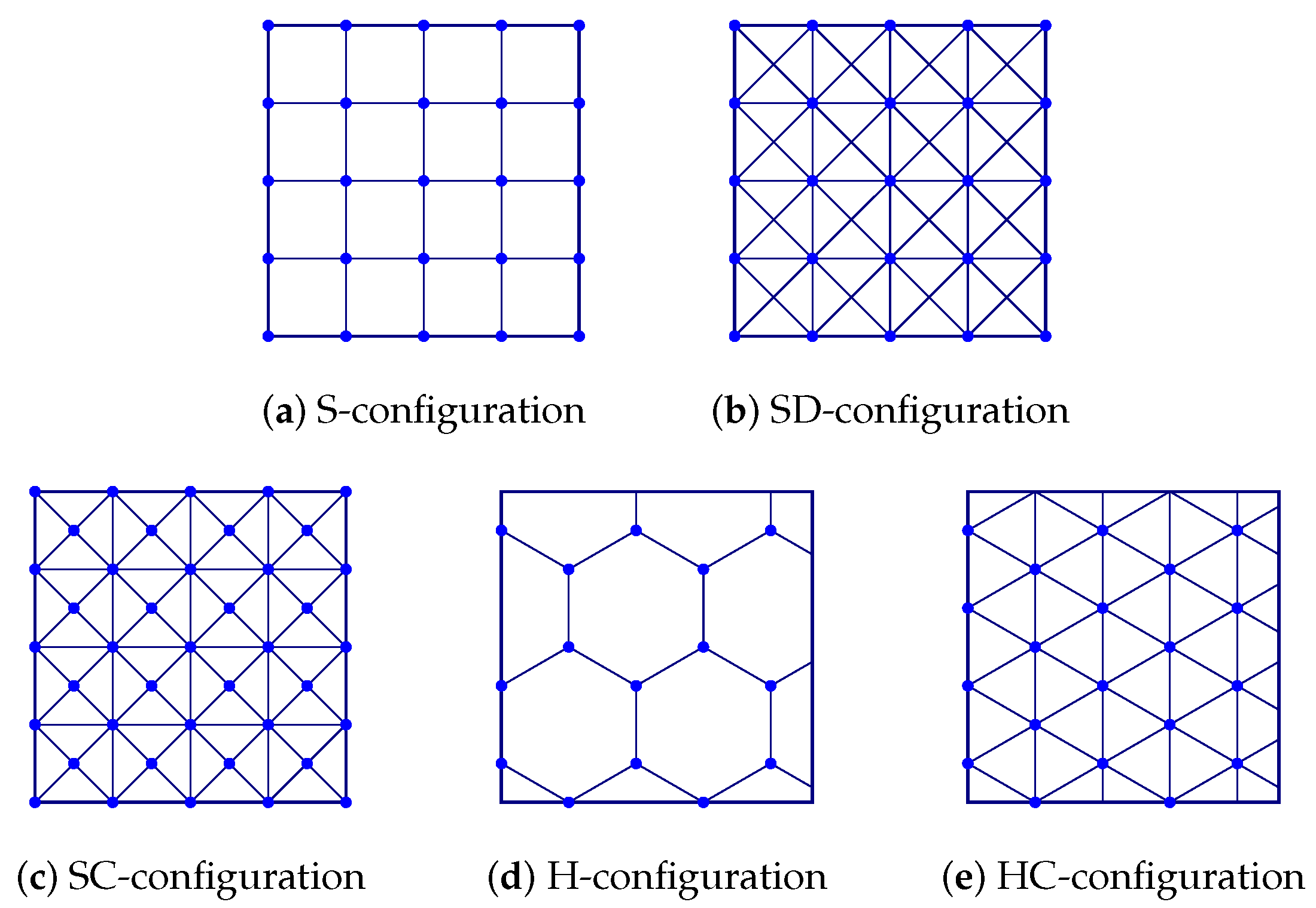
RGPPM is a novel emerging alternative for planning trajectories from a start point to an end point. This methodology has been successfully evaluated for the movement of terrestrial robotic systems [17,18]. However, until now, configuration spaces with regular geometrical patterns have been exclusively explored, as shown in Figure 1.

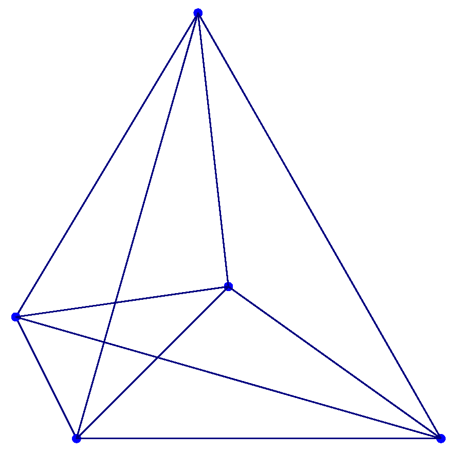
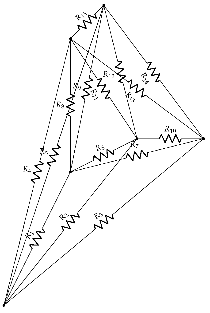
In order to expand RGPPM for planning merchandise deliveries, it is necessary to establish configuration spaces with multi-connected irregular geometrical patterns, as shown in Figure 2. This configuration represents a novel contribution in research with the purpose of merging path planning and merchandise deliveries using geometrical patterns.

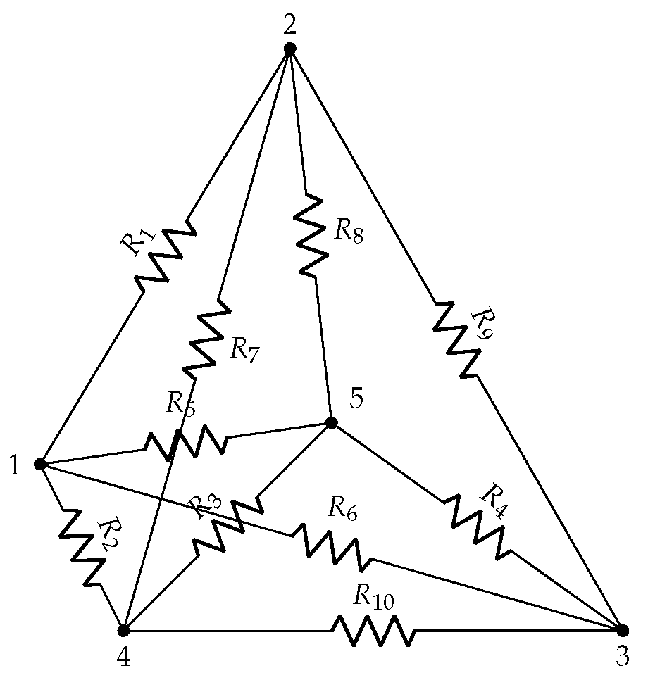
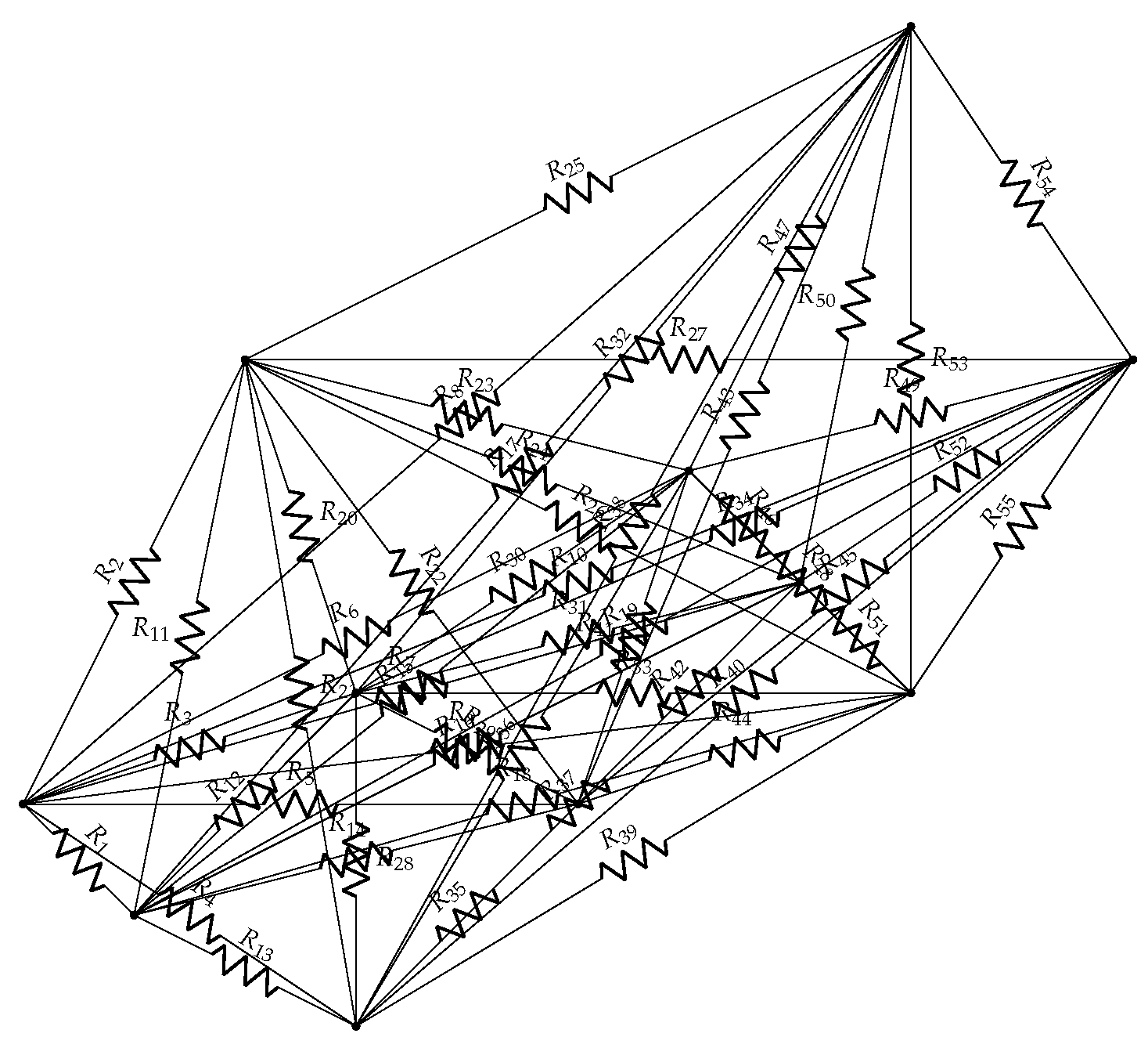
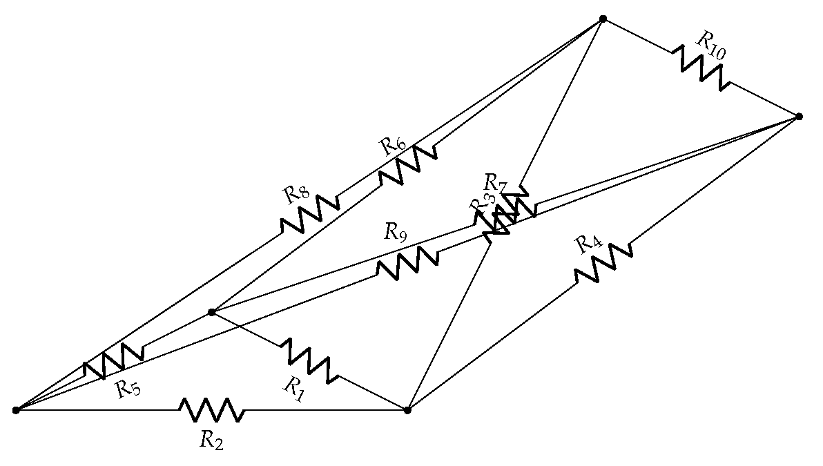
As it can be seen, the nodes have been fully connected to each other and therefore the edges represent all possible connections between nodes. If it is assumed that each node represents a position to deliver merchandise, then the edges describe the paths between the different destinations. Subsequently, the modeling of the configuration space using resistive grids is carried out, as shown in Figure 3. In the same way that it has been shown previously, this configuration represents a novel contribution in research with the purpose of merging path planning and merchandise deliveries using resistive grids.

According to the irregular geometrical configuration of Figure 2, the values of the edges are related to the length between the nodes and therefore the values of the resistors in Figure 3, $R_1$, $R_2$, $R_3$, $R_4$, $R_5$, $R_6$, $R_7$, $R_8$, $R_9$, and $R_{10}$ are related to the length of the paths between locations of handing over $\left\{1,2,3,4,5\right\}$.

With the purpose of carrying out a simple example, the resistive grid in Figure 3 has been characterized by the resistor values shown in

Table 1. Resistor values for the multi-connected grid configuration.

Resistor	Value $\mathbf{\Omega }$
$R_1$	5.83
$R_2$	2.23
$R_3$	3.53
$R_4$	4.30
$R_5$	3.53
$R_6$	7.28
$R_7$	7.28
$R_8$	4.52
$R_9$	8.06
$R_{10}$	6.00

. These values have been calculated by locating the nodes on a Cartesian plane and measuring the distance between each one.

After establishing values for resistors in Figure 3, it is necessary to connect power supplies on all nodes in the resistive grid. In order to do this, $E_1$, $E_2$, $E_3$, $E_4$, and $E_5$ power supplies have been connected to nodes $\left\{1,2,3,4,5\right\}$, respectively. It is important to determine which is the node of the starting delivery for assigning to the power supply located in that position a value different from 0 V. In this case, $E_1$ = 10 V, and from $E_2$ to $E_5$, it is equal to 0 V. It is important to mention that the above numerical value of $E_1$ has been established for the purpose of carrying out a simple example since all positive values are considered feasible.

When the characterization of the resistive grid has been achieved, the Modified Nodal Analysis (MNA) [19] procedure is carried out in order to formulate the equilibrium equations. Therefore, conductance and independent voltage source stamps [20,21] are carried out as follows:

$$\begin{array}{cccc}& v_i& v_j& \mathrm{RHS}\\ i& G& -G& 0\\ j& -G& G& 0\end{array}$$

(1)

$$\begin{array}{ccccc}& v_i& v_j& i_E& \mathrm{RHS}\\ i& 0& 0& +1& 0\\ j& 0& 0& -1& 0\\ \mathrm{BE}& +1& -1& 0& E\end{array}$$

(2)

where $v_i$ and $v_j$ represent the nodal voltage with respect to ground, i and j are the nodes of the elements, E is the supplied voltage by the independent voltage source (IVS), $G=\frac{1}{R}$ is the equivalent conductance, RHS means the right-hand side of the equilibrium equation, and $i_E$ is the unknown current that crosses by the IVS.

According to Equations (1) and (2), the formulation of the linear system of equations in Figure 3 is based on the form $Ax=b$ as follows:

$$A=\left[\begin{array}{cccccccccc}1.04& -0.17& -0.13& -0.44& -0.28& 1& 0& 0& 0& 0\\ -0.17& 0.65& -0.12& -0.13& -0.22& 0& 1& 0& 0& 0\\ -0.13& -0.12& 0.66& -0.16& -0.23& 0& 0& 1& 0& 0\\ -0.44& -0.13& -0.16& 1.03& -0.28& 0& 0& 0& 1& 0\\ -0.28& -0.22& -0.23& -0.28& 1.02& 0& 0& 0& 0& 1\\ 1& 0& 0& 0& 0& 0& 0& 0& 0& 0\\ 0& 1& 0& 0& 0& 0& 0& 0& 0& 0\\ 0& 0& 1& 0& 0& 0& 0& 0& 0& 0\\ 0& 0& 0& 1& 0& 0& 0& 0& 0& 0\\ 0& 0& 0& 0& 1& 0& 0& 0& 0& 0\end{array}\right]$$

$$x=\left[\begin{array}{c}{v}_1\\ v_2\\ v_3\\ v_4\\ v_5\\ i_{E_1}\\ i_{E_2}\\ i_{E_3}\\ i_{E_4}\\ i_{E_5}\end{array}\right]b=\left[\begin{array}{c}0\\ 0\\ 0\\ 0\\ 0\\ 10\\ 0\\ 0\\ 0\\ 0\end{array}\right]$$

where A is a sparse matrix (MNA matrix), and x and b are vectors (unknowns and stimulus vector, respectively). It is important to mention that RGPPM uses a direct method for solving systems of linear equations called a multifrontal method from Unsymmetric MultiFrontal PACK (UMFPACK) [22].

After carrying out the multifrontal method in the linear system of equations, the solutions are shown in

Table 2. Summary of voltages and currents.

Variable	Value
$v_1$	10.0 V
$v_2$	0 V
$v_3$	0 V
$v_4$	0 V
$v_5$	0 V
$i_{E_1}$	−10.4 A
$i_{E_2}$	1.7 A
$i_{E_3}$	1.3 A
$i_{E_4}$	4.4 A
$i_{E_5}$	2.8 A

.

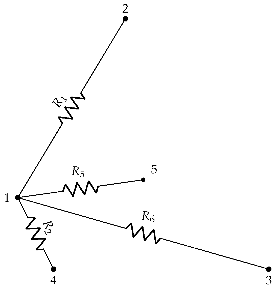
With the values of the nodal voltages, the next step consists of finding the path from the starting delivery to the new position of the next delivery. In order to do this, RGPPM uses a Local Current Comparison (LCC) [23] algorithm for calculating the branch currents and therefore it establishes the largest branch current.

According to Figure 4, the LCC algorithm starts at node one. Firstly, it determines the neighboring nodes to the actual node $\left\{2,3,4,5\right\}$. Then, it calculates the branch currents to neighboring nodes using the following expression:

$$I_j=\frac{V-V_n}{R_j}$$

(3)

where $R_j$, $V_n$, V, and $I_j$ represent the resistance value in the j-branch, the voltage of the neighboring node in the j-branch, the actual nodal voltage, and the current in the j-branch, respectively.

Table 3. Branch currents from Figure 4.

Current	Value
$i_{R_1}$	1.71 A
$i_{R_5}$	2.83 A
$i_{R_6}$	1.37 A
$i_{R_2}$	4.48 A

shows the currents of the branches connected to node one. According to this list of values, the highest current flows through resistor $R_2$ and therefore this branch must be considered as the path to the new actual node $\left\{4\right\}$.

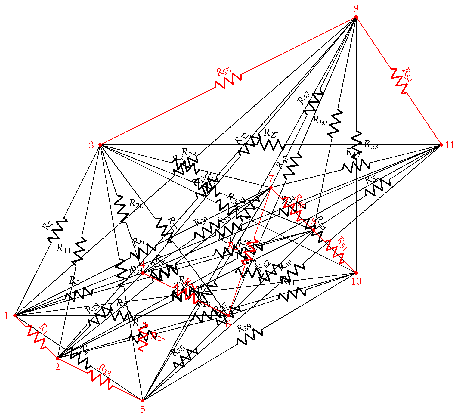
After that, the previous node and the branches connected to it should be removed from the multi-connected resistive grid configuration before continuing with the new actual node. However, the previous node and the branch of the highest current connected to it must be stored because these elements belong to the complete path for merchandise deliveries.

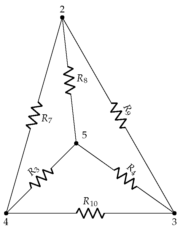
Figure 5 shows the modified multi-connected resistive grid configuration after removing the previous node and the branches connected to it. Finally, with this new multi-connected resistive grid configuration, the stages of assigning power supplies to the nodes, the formulation of the equilibrium equations, the solution of the system of equations, the path search procedure and the modification of the resistive grid configuration must be carried out again and repeatedly until all positions for delivering merchandise have been passed.

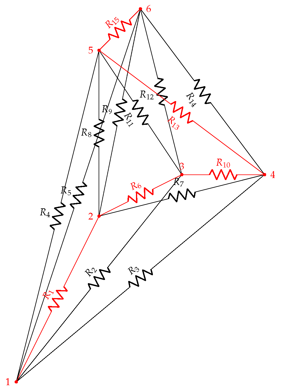
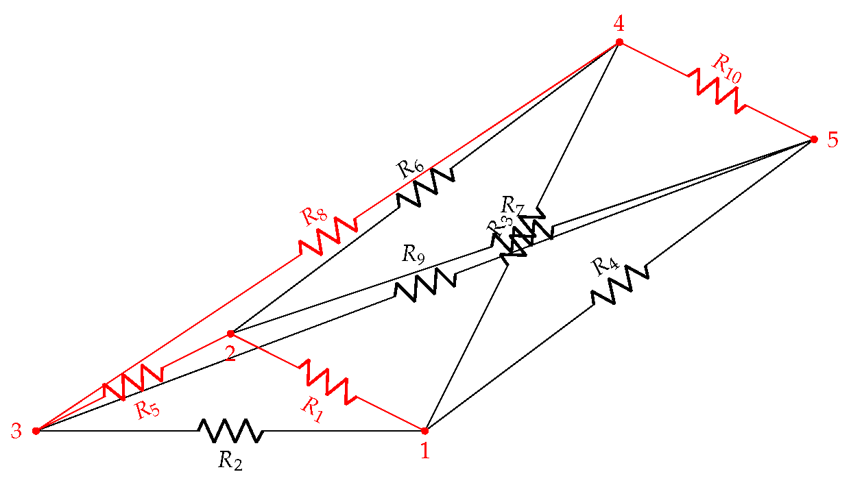
As can be seen in Figure 6, the resistors in red $\left\{R_2,R_3,R_4,R_9\right\}$ form a connection tree with all the nodes of the resistive grid and therefore it is possible to establish the complete path for delivering merchandise. In addition, the sequence of nodes in the complete path $\left\{1,4,5,3,2\right\}$ represents the sequence of positions in order to deliver merchandise. In addition, the sum of the resistor values represents the total length of the path for delivering merchandise; for this example, it is 18.12.

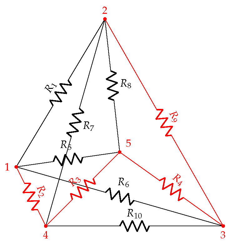
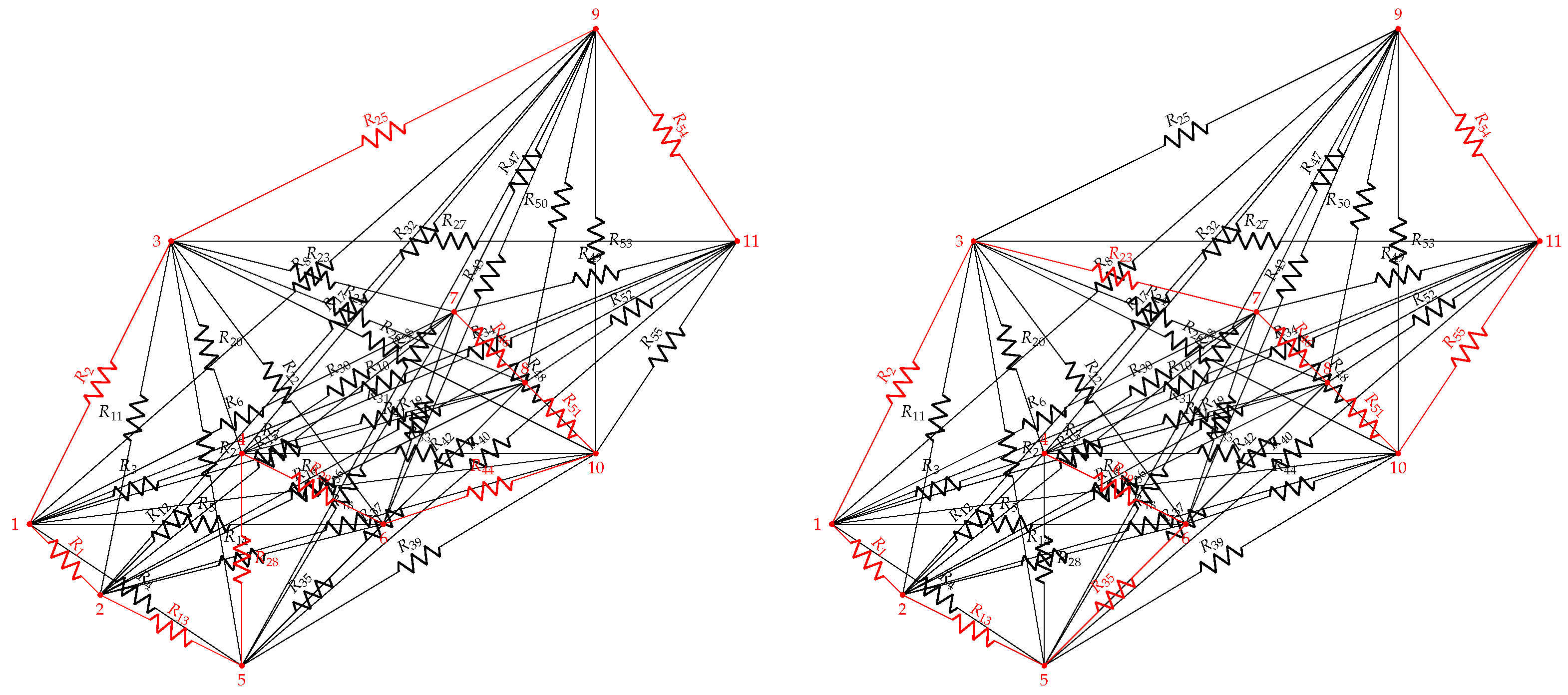
It is important to mention that, for this example, the starting point to deliver merchandise has been established at node one and therefore the route sequence is $\left\{1,4,5,3,2\right\}$. However, the technique is capable of modifying the starting node to a different point and thus it generates a new tree connection with all nodes.

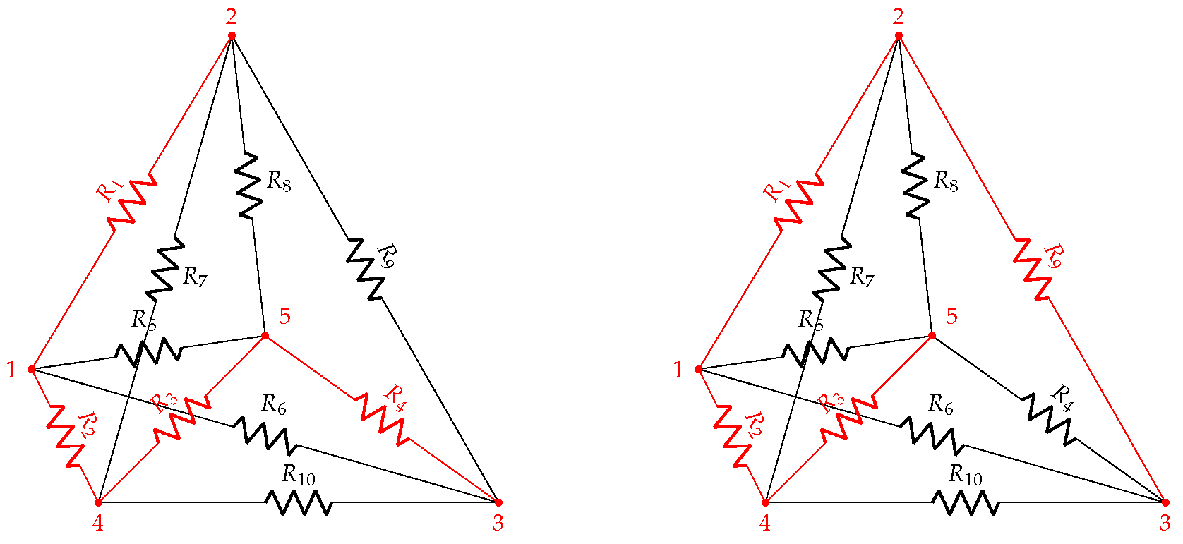
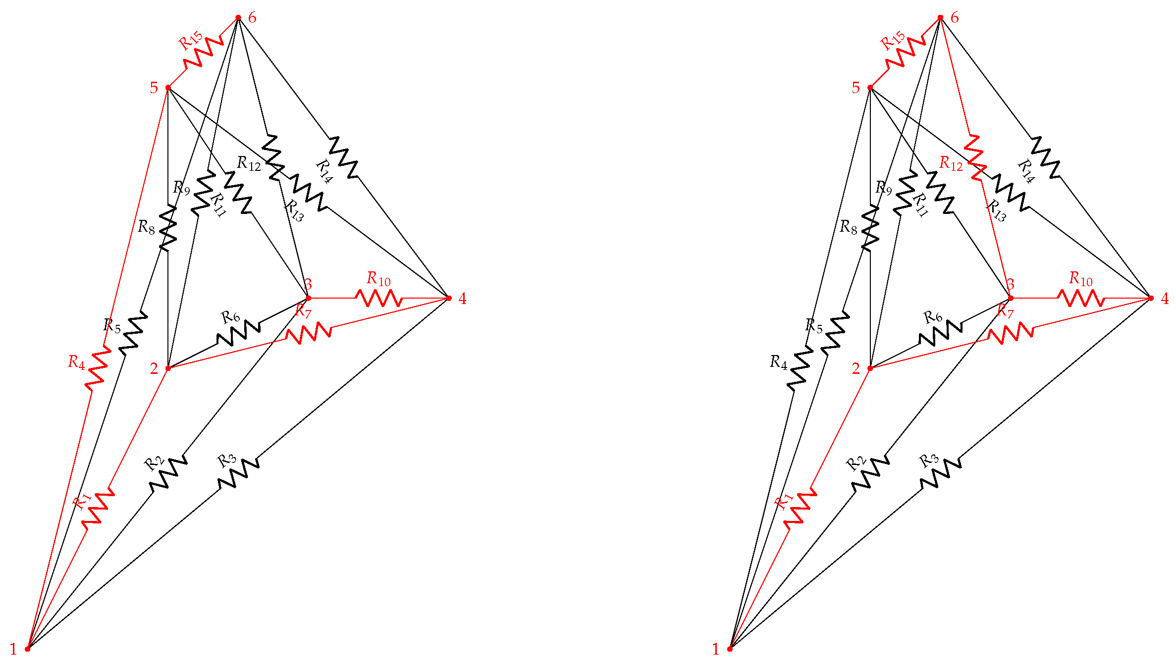
Figure 7 shows two alternate full path resistive grid configurations using different starting nodes. In the case of the resistive grid on the left side, the starting node is the number three which generates a connection tree formed by the resistors in red $\left\{R_4,R_3,R_2,R_1\right\}$ and a path sequence $\left\{3,5,4,1,2\right\}$. On the other hand, the resistive grid on the right side starts at node five generating a connection tree compound of the resistors in red $\left\{R_3,R_2,R_1,R_9\right\}$ and a path sequence $\left\{5,4,1,2,3\right\}$. In addition, the total lengths of each path shown in left-side and right-side Figure 7 are 15.89 and 19.65, respectively.

With the change of starting node, the possibility of exploring the different starting points in the resistive grid is opened, and therefore it is possible to determine which is the connection tree that reduces the total distance for the path between all the nodes of the resitive grid. Particularly, for this example, five different connection trees can be generated by changing the starting node.

Table 4. Performance of the paths from Figure 3 by changing the start node.

Starting Node	Sequence of Nodes Using RGPPM	Length
1	$\left\{1,4,5,3,2\right\}$	18.12
2	$\left\{2,5,1,4,3\right\}$	16.28
3	$\left\{3,5,4,1,2\right\}$	15.89
4	$\left\{4,1,5,3,2\right\}$	18.12
5	$\left\{5,4,1,2,3\right\}$	19.65

shows the five possible starting points for delivering merchandise. Based on the results for the length of the path that passes through all the nodes, the choice of node three as the starting point is the most convenient due to its smaller value.

3. Experimental Results

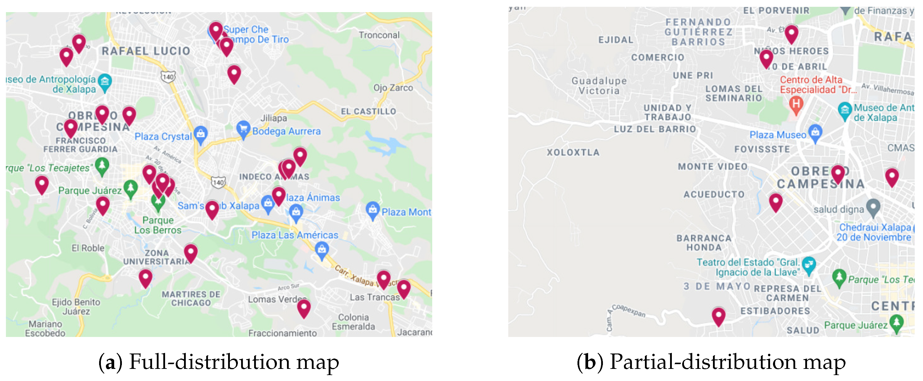
With the purpose of evaluating the feasibility of the RGPPM extension in order to deliver merchandise, Lecheria y Quesos Artesanales “Los Ángeles” has shared three maps of the locations for the deliveries of its products from three different cities: Puebla, Xalapa, and Veracruz-Boca del Rio. In these maps, the locations are transformed into nodes belonging to multi-connected resistive grid configurations in order to carry out the modified RGPPM algorithm and therefore establish the complete path for delivering merchandise.

For each experimental case, a partial distribution zone has been established in order to carry out the technique based on resistive grids. In addition, the search of two alternative full path resistive grid configurations have been explored using different starting nodes. Finally, the behavior of the computation time as the number of georeferential locations increases has been evaluated.

3.1. Puebla Logistical Map

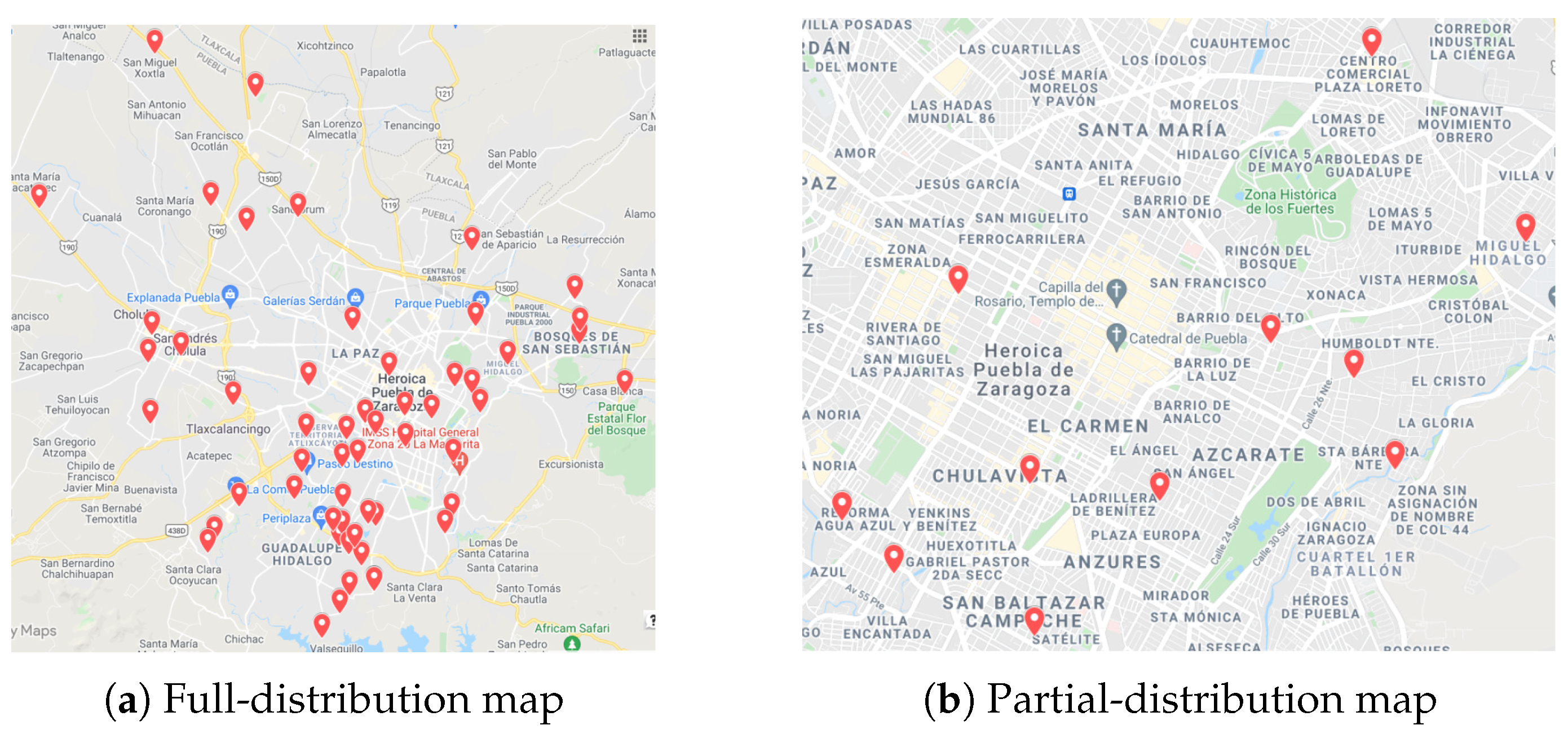
In the city of Puebla, Lecheria y Quesos Artesanales “Los Ángeles” distributes its merchandise to the locations of fifty-four customers, as shown in Figure 8a. As it can be seen, the distribution of the merchandise delivery points contains disperse and concentrate areas.

With the purpose of showing the transformation from the distribution map to the resistive grid, a partial distribution zone has been selected as shown in Figure 8b. This set of eleven georeferential locations has been converted into a multi-connected resistive grid, as shown in Figure 9.

As it can be seen, the eleven geopositions have been interconnected by fifty-five resistors. In order to assign numerical values to resistors, it is necessary to calculate the distance between pairs of georeferential coordinates. In this part of the experimental results, the distance between two points on the earth’s surface has been estimated using the mathematical approximation of the Harvesine formula [24]

$$d=2rarcsin\left(\sqrt{{sin}^2\left({\displaystyle \frac{{\varphi }_2-{\varphi }_1}{2}}\right)+cos\left({\varphi }_1\right)cos\left({\varphi }_2\right){sin}^2\left({\displaystyle \frac{{\lambda }_2-{\lambda }_1}{2}}\right)}\right)$$

(4)

where ${\varphi }_1$, ${\varphi }_2$, ${\lambda }_1$, ${\lambda }_2$ are the latitude and longitude, expressed in radians, of the first and second georeferential points, respectively, and r is the terrestrial radius (6371 km approx.)

It is important to mention that the Haversine expression is more accurate for calculating longer distances between two points on the surface than two-dimensional Euclidean distances due to consideration of the curvature of the earth. Therefore, this addition opens the possibility to explore multi-connected irregular geometrical grid configurations with the greatest possible dispersion between customer locations.

After carrying out Equation (4), the distances between all the pairs of locations of the merchandise deliveries have been calculated and therefore the numerical values (in $\mathsf{\Omega }$) of the fifty-five resistors for the multi-connected resistive grid from Puebla map have been established as shown in

Table 5. Resistor values for the Puebla map.

Resistor	Value	Resistor	Value	Resistor	Value	Resistor	Value	Resistor	Value
$R_1$	0660	$R_{12}$	1460	$R_{23}$	2840	$R_{34}$	4950	$R_{45}$	4030
$R_2$	2280	$R_{13}$	1380	$R_{24}$	3630	$R_{35}$	1650	$R_{46}$	0810
$R_3$	1720	$R_{14}$	2470	$R_{25}$	4280	$R_{36}$	3360	$R_{47}$	2730
$R_4$	2010	$R_{15}$	3960	$R_{26}$	4220	$R_{37}$	3680	$R_{48}$	1590
$R_5$	2850	$R_{16}$	4490	$R_{27}$	5110	$R_{38}$	6010	$R_{49}$	2470
$R_6$	4150	$R_{17}$	6310	$R_{28}$	1360	$R_{39}$	3560	$R_{50}$	2880
$R_7$	4770	$R_{18}$	4590	$R_{29}$	1170	$R_{40}$	5650	$R_{51}$	0900
$R_8$	6310	$R_{19}$	6400	$R_{30}$	2490	$R_{41}$	1720	$R_{52}$	1970
$R_9$	4980	$R_{20}$	1820	$R_{31}$	3060	$R_{42}$	2070	$R_{53}$	3710
$R_{10}$	6620	$R_{21}$	3140	$R_{32}$	4900	$R_{43}$	4410	$R_{54}$	2160
$R_{11}$	2570	$R_{22}$	2580	$R_{33}$	3280	$R_{44}$	2140	$R_{55}$	2360

.

Hereinafter, the modified version of RGPPM begins iteratively searching for the path that goes through all the locations for delivering merchandise.

According to Figure 10, the path through the eleven locations for delivering merchandise contains the resistors in red $\left\{R_1,R_{13},R_{28},R_{28},R_{41},R_{46},R_{51},R_{55},R_{54},R_{25}\right\}$ and the sequence of nodes in the complete path is $\left\{1,2,5,4,6,7,8,10,11,9,3\right\}$. Moreover, the total length of the path is 16.88 km.

Figure 11 shows two alternate full path resistive grid configurations using different starting nodes. In the case of the resistive grid on the left side, the starting node is the number seven, which generates a connection tree formed by the resistors in red $\left\{R_{46},R_{51},R_{44},R_{29},R_{28},R_{13},R_1,R_2,R_{25},R_{54}\right\}$ and a path sequence $\left\{7,8,10,6,4,5,2,1,3,9,11\right\}$. On the other hand, the resistive grid on the right side starts at node four generating a connection tree compound of the resistors in red $\left\{R_{29},R_{35},R_{13},R_1,R_2,R_{23},R_{46},R_{51},R_{55},R_{54}\right\}$ and a path sequence $\left\{4,6,5,2,1,3,7,8,10,11,9\right\}$. In addition, the total lengths of each path shown on the left-side and the right-side Figure 11 are 17.14 km and 16.21 km, respectively.

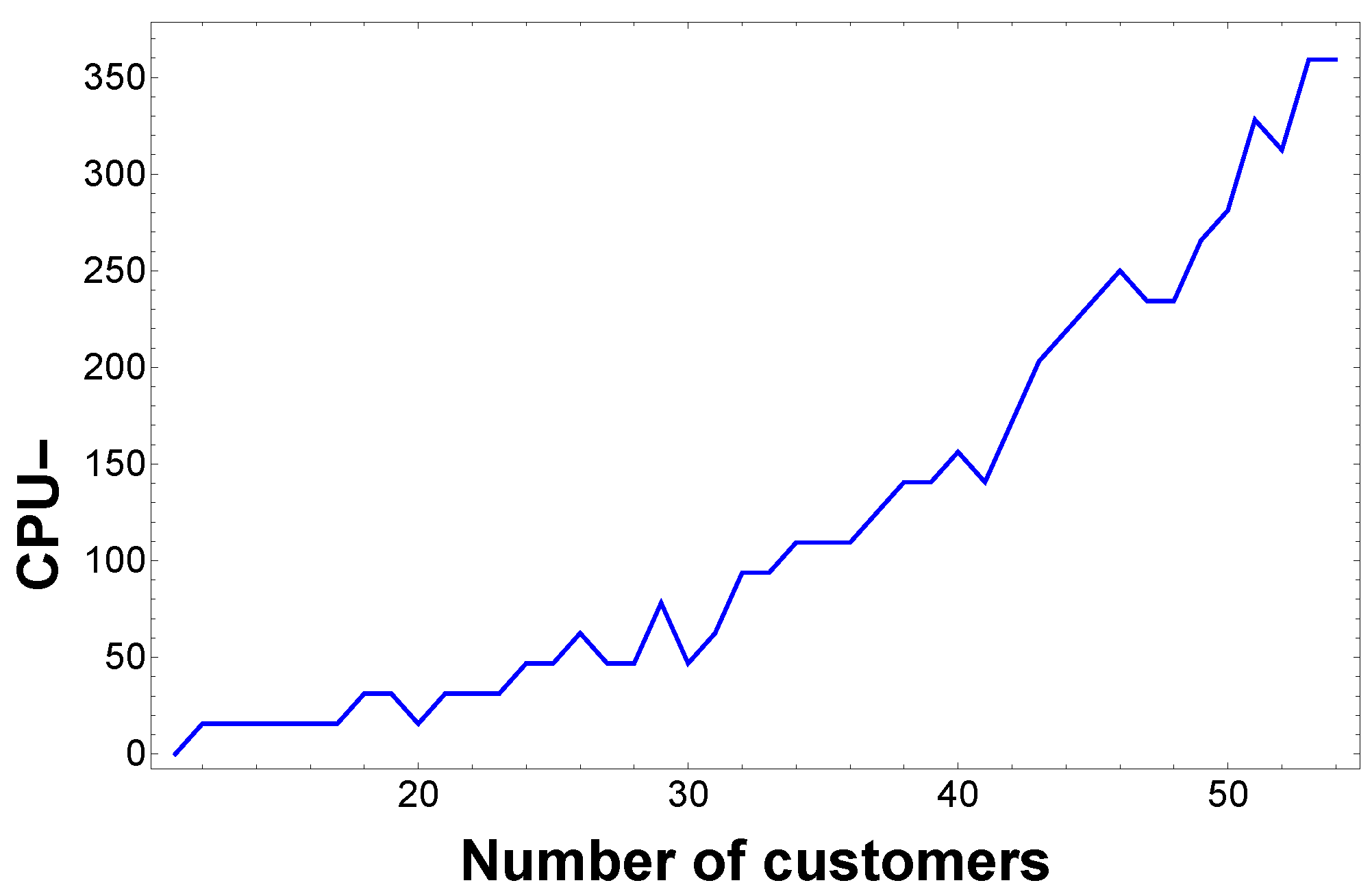
As it can be seen in Figure 12, the behavior of the CPU-time with respect to the number of merchandise delivery points has been successfully estimated. Start from the partial distribution zone (seven customers), the computation time, in order to transform the georeferential locations into a resistive grid, formulate the equilibrium equations, solve the system of equations, and find the path that runs through all the nodes that has been established according to increases in the number of customers by one until the maximum amount (fifty-four customers) has been achieved.

It is important to mention that, as the number of customers increases, the CPU-time increases, with the maximum computation time reached around 360 ms.

3.2. Xalapa Logistical Map

In the city of Xalapa, Lecheria y Quesos Artesanales “Los Ángeles” distributes its merchandise to the locations of twenty-five customers, as shown in Figure 13a. In the same way as in the city of Puebla, the location of the customers displays concentrated and disperse areas.

Figure 13b shows the partial distribution zone in order to be transformed from the distribution map to the resistive grid. In order to do this, the six georeferential locations have been converted into a multi-connected resistive grid, as shown in Figure 14.

After having converted the georeference locations into a multi-connected resistive grid, it is necessary to carry out the mathematical expression shown in Equation (4) in order to estimate the numerical values (in $\mathsf{\Omega }$) of the fifteen resistors as shown in

Table 6. Resistor values for Xalapa map.

Resistor	Value	Resistor	Value	Resistor	Value
$R_1$	1620	$R_6$	0870	$R_{11}$	1730
$R_2$	2370	$R_7$	1510	$R_{12}$	1890
$R_3$	2830	$R_8$	1840	$R_{13}$	2200
$R_4$	3340	$R_9$	2170	$R_{14}$	2240
$R_5$	3720	$R_{10}$	0680	$R_{15}$	1470

.

From this moment, the formulation of the equilibrium equations, the solution of the system of equations, and the path search procedure are carried out for establishing the path that goes through all the locations for delivering merchandise.

According to Figure 15, the path through the six locations for delivering merchandise contains the resistors in red $\left\{R_1,R_6,R_{28},R_{10},R_{13},R_{15}\right\}$ and a path sequence $\left\{1,2,3,4,5,6\right\}$. Therefore, it reaches a total distance of 6.84 km.

Figure 16 shows two alternate full path resistive grid configurations using different starting nodes. In the case of the resistive grid on the left side, the starting node is the number three, which generates a connection tree formed by the resistors in red $\left\{R_{10},R_7,R_1,R_4,R_{15}\right\}$ and a path sequence $\left\{3,4,2,1,5,6\right\}$. On the other hand, the resistive grid on the right side starts at node five generating a connection tree compound of the resistors in red $\left\{R_{15},R_{12},R_{10},R_7,R_1\right\}$ and a path sequence $\left\{5,6,3,4,2,1\right\}$. Moreover, the total lengths of each path shown on the left-side and right-side (Figure 16) are 8.62 km and 7.17 km, respectively.

With the same purpose as in the city of Puebla, the information in

Table 7. Performance of CPU-time for different amounts of customers in the Xalapa map.

Number of Customers	CPU-Time (ms)	Number of Customers	CPU-Time (ms)
6	15.62	16	15.62
7	15.62	17	31.25
8	15.62	18	31.25
9	15.62	19	31.25
10	15.62	20	31.25
11	15.62	21	31.25
12	15.62	22	31.25
13	15.62	23	31.25
14	15.62	24	46.87
15	15.62	25	46.87

shows that, as the number of customers increases, the computation time remains constant in most of the range of variation. The maximum computation time reached is 46.87 ms.

3.3. Veracruz-Boca del Rio Logistical Map

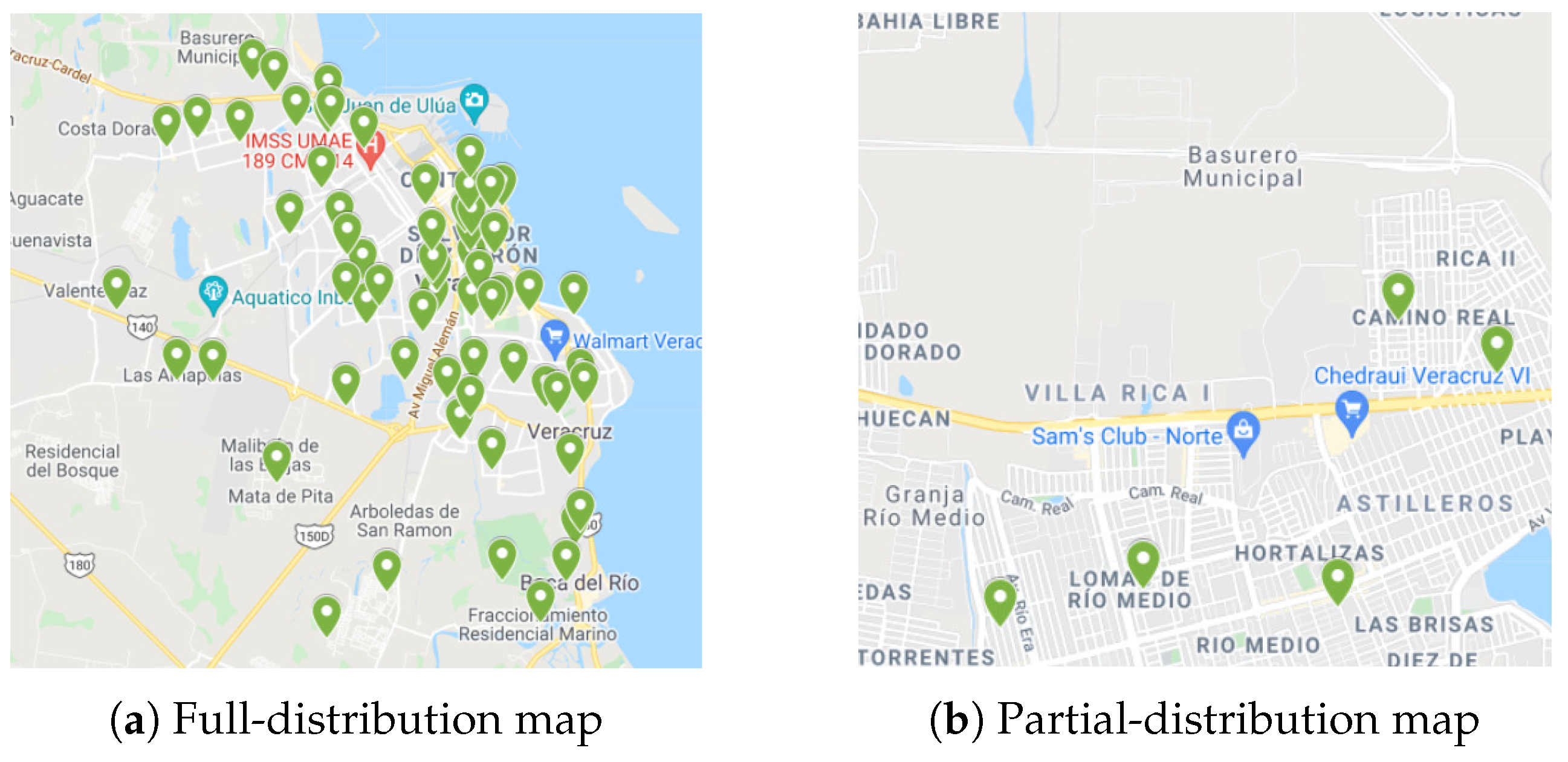
In the Veracruz-Boca del Rio metropolitan area, Lecheria y Quesos Artesanales “Los Ángeles” distributes its merchandise to the locations of sixty-four customers, as shown in Figure 17a.

In the same way that it has been carried out previously, a partial distribution zone is transformed into a resistive grid by converting five georeferential locations to a multi-connected resistive grid as shown in Figure 18.

Table 8. Resistor values for the Veracruz-Boca del Rio map.

Resistor	Value	Resistor	Value
$R_1$	1060	$R_6$	2010
$R_2$	1830	$R_7$	2250
$R_3$	1590	$R_8$	2730
$R_4$	1530	$R_9$	3020
$R_5$	0800	$R_{10}$	0600

shows the numerical values (in $\mathsf{\Omega }$) of the ten resistors calculated with the mathematical expression shown in Equation (4).

Next, the extension of RGPPM for green logistics is carried out in order to establish the path that passes through all the locations for delivering merchandise. Figure 19 shows the path through the five locations for delivering merchandise. It contains the resistors in red $\left\{R_1,R_5,R_8,R_{10}\right\}$, the path sequence $\left\{1,2,3,4,5\right\}$, and therefore reaches a total distance of 5.19 km.

According to the steps previously carried out in the maps of the cities of Puebla and Xalapa, the exploration of the alternate full path resistive grid configurations using different starting nodes and the behavior of the computation time as the number of clients increases must be accomplished. However, these results have not been shown because they are similar to the previous cases.

Finally, the experimental results confirm, through the exploration of three logistics maps for the delivery of merchandise from Lecheria y Quesos Artesanales “Los Ángeles” business, that the novel green logistic technique based on RGPPM extension is capable of establishing path trees connected to all georeferential points. Additionally, it has been shown that the technique is capable of changing the starting point and therefore re-generating new alternatives in order to deliver merchandise. Moreover, it has been possible to observe the behavior of the computing time as the number of clients increases.

4. Discussion

Although the research does not intend to carry out a numerical comparison between the traditional methods or techniques of easy computational implementation for the delivery of merchandise and the novel technique based on RGPPM, it is convenient to discuss the similarities and differences with respect to the principal characteristics of each technique. According to the experience of the authors and as far as the knowledge about the area reaches, it is possible to consider two fundamental methods: Dijkstra [25] and Kruskal [26] algorithms.

The classical Dijkstra algorithm [27] solves the single origin shortest path problem on a weighted graph. Because the problem of delivering merchandise to all hand-over points during the shortest continuous path is related to the connection of a weighted graph, Dijkstra’s algorithm can be considered as an alternative to attack this problem. However, the shortest path between two locations is not the same as the minimum spanning tree that connects all hand-over points in a continuous path. Therefore, Dijkstra’s original conception must be modified to address the search for the minimum weight spanning tree. At this point, it is important to mention that RGPPM has previously shown to be able to estimate the shortest path from one point to another for weighted graphs from resistive grids and as a consequence of the present investigation RGPPM can be expanded towards the problem of the search for the minimum spanning tree. Due to this, RGPPM represents an advantage since it is capable of tackling two different problems with the same original conception of the algorithm.

The Kruskal algorithm [28] generates a spanning tree with a minimal cost for the sum of all edge weights, i.e., a minimum spanning tree. However, this algorithm has been considered short-sighted for its estimates since it makes decisions using the available information without worrying about the effect that these decisions may cause in the future and therefore many problems may not have been solved correctly. According to the methodological structure of RGPPM, it is possible to establish an advantage compared to the Kruskal method because RGPPM uses the MNA formulation to concentrate all the information of the weighted graph in the form of a resistive grid and therefore be able to estimate the changes in the grid using theorems from circuit theory. This feature causes a focus-sighted in order to carry out decisions.

According to Figure 3, the multi-connected resistive grid configuration is capable of containing twenty-four different paths in order to traverse the locations for delivering merchandise.

Table 9. Performance of the paths from Figure 3.

Path	Sequence of Nodes	Length
1	$\left\{1,2,3,4,5\right\}$	23.42
2	$\left\{1,2,3,5,4\right\}$	21.72
3	$\left\{1,2,4,3,5\right\}$	23.41
4	$\left\{1,2,4,5,3\right\}$	20.94
5	$\left\{1,2,5,3,4\right\}$	20.65
6	$\left\{1,2,5,4,3\right\}$	19.88
7	$\left\{1,3,2,4,5\right\}$	26.15
8	$\left\{1,3,2,5,4\right\}$	23.39
9	$\left\{1,3,4,2,5\right\}$	25.08
10	$\left\{1,3,4,5,2\right\}$	21.33
11	$\left\{1,3,5,2,4\right\}$	23.38
12	$\left\{1,3,5,4,2\right\}$	22.39
13	$\left\{1,4,2,3,5\right\}$	21.87
14	$\left\{1,4,2,5,3\right\}$	18.33
15	$\left\{1,4,3,2,5\right\}$	20.81
16	$\left\{1,4,3,5,2\right\}$	17.05
17	$\left\{1,4,5,2,3\right\}$	18.34
18	$\left\{\mathbf{1},\mathbf{4},\mathbf{5},\mathbf{3},\mathbf{2}\right\}$	18.12
19	$\left\{1,5,2,3,4\right\}$	22.11
20	$\left\{1,5,2,4,3\right\}$	21.33
21	$\left\{1,5,3,2,4\right\}$	23.17
22	$\left\{1,5,3,4,2\right\}$	21.11
23	$\left\{1,5,4,2,3\right\}$	22.40
24	$\left\{1,5,4,3,2\right\}$	21.12

shows the paths, the sequence of nodes, and the length of the path.

As it can be seen in the previous table, the path established by RGPPM contains the sequence of nodes $\left\{\mathbf{1},\mathbf{4},\mathbf{5},\mathbf{3},\mathbf{2}\right\}$ and therefore the length of the path is 18.12. Because the length of the path is related to the displacement of a terrestrial vehicle for delivering merchandise, it is possible to assert that RGPPM reduces the total distance of the path by around 30% compared to the longest path. Moreover, it is important to mention that reducing the length of the path has a considerable impact on different variables such as: amount of fuel, travel time, and emission of pollutants.

Based on simulation results, it is possible to determine that the location of the starting node on the multi-connected resistive grid is a fundamental piece for the length of the path in order to deliver merchandise.

Table 10. Performance of the paths from Figure 3 by changing the start node.

Starting Node	Sequence of Nodes Using RGPPM	Porcentage of Reduction
1	$\left\{1,4,5,3,2\right\}$	30.70%
2	$\left\{2,5,1,4,3\right\}$	32.42%
3	$\left\{3,5,4,1,2\right\}$	44.47%
4	$\left\{4,1,5,3,2\right\}$	30.70%
5	$\left\{5,4,1,2,3\right\}$	24.85%

shows the length of the paths and the percentage of reduction with respect to the longest path as the starting node changes in Figure 3.

As it can be seen in the table above, the reduction in the length of the path for delivering merchandise undergoes significant changes for different starting nodes. For example, the difference in percentage between the shortest path and the longest path during changes in the starting node has been estimated from 25% to 45%. Therefore, it is possible to reduce or increase the displacement path of a transport system for delivering merchandise by changing the initial location.

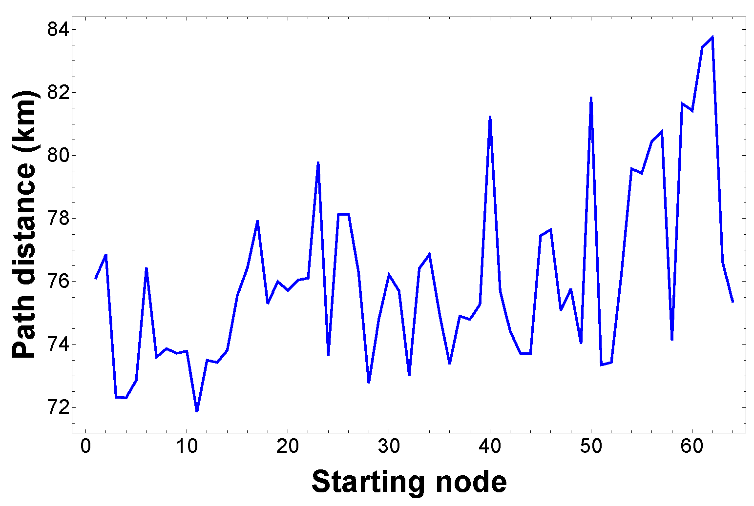
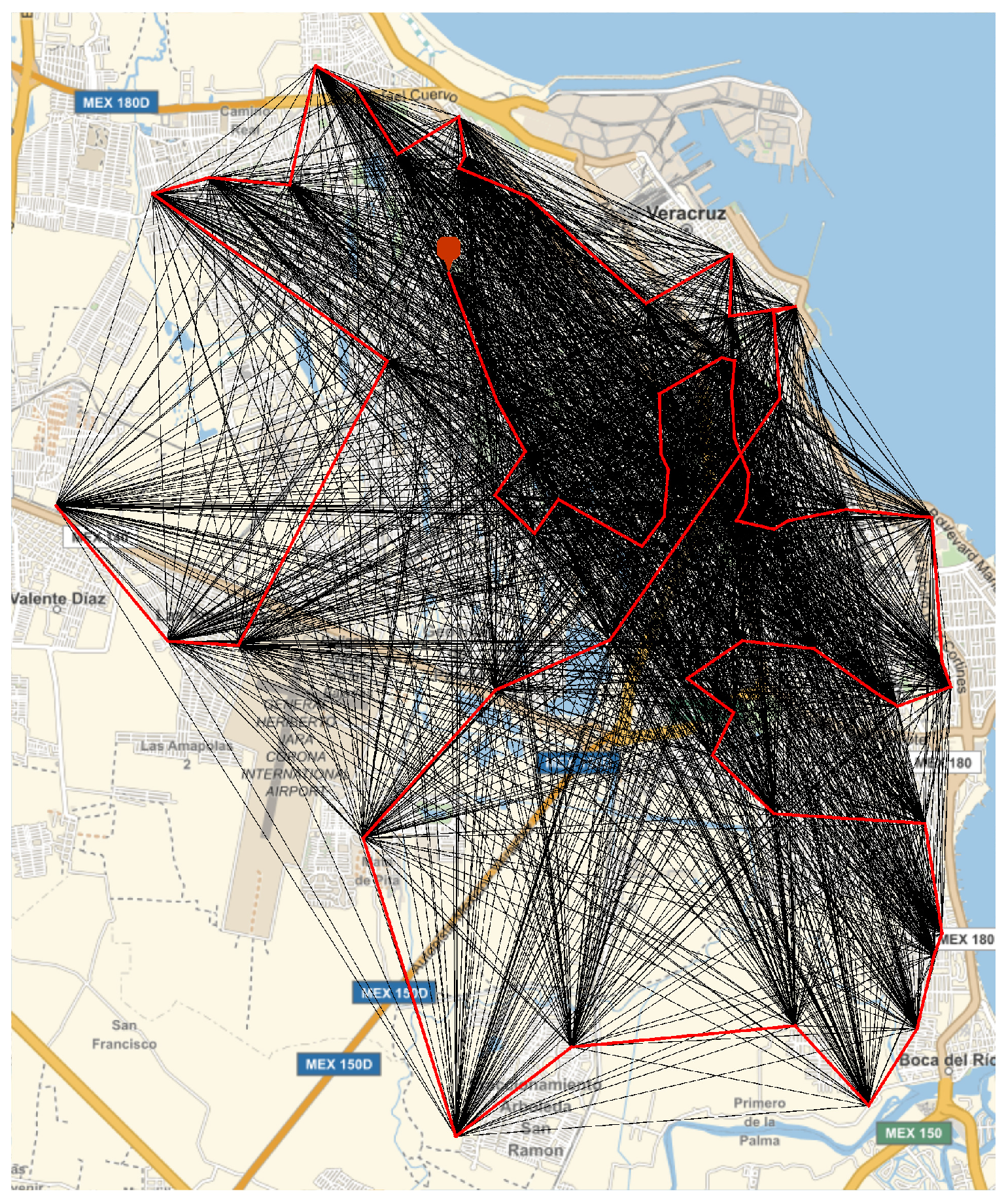
A strategical and decisive factor for the success or failure of a business is the location of a merchandise distribution center. According to experimental results from the RGPPM-based technique, it is possible to glimpse the feasible positions for locating a merchandise distribution center, as shown in Figure 20.

Figure 20 shows the complete distance for delivering merchandise by changing the start node. According to these results, it is possible to establish that the maximum distance is around 84 km, and the minimum distance is around 72 km. However, there are thirteen different starting nodes where the complete distance to deliver merchandise remains close to the minimum distance. It is important because it opens up the possibility of various alternatives for the location of a merchandise distribution center.

For the purpose of evidencing the feasibility of this new technique, in order to recalculate the tree connection with all the nodes based on the estimation of the best place to locate a merchandise distribution center, Figure 21 shows the multiconnected resistive grid (black lines), the actual location of the merchandise distribution center (orange marker), and the shortest path for delivering merchandise (red lines).

Figure 12 and Table 7 have shown the evolution of the computation time as the number of merchandise delivery points increases. Despite of observing that the CPU-time tends to increase as the number of georeferential points increases in the logistic map of the cities, it is possible to agree that the behavior of the curve and the data reflect a smooth nonlinear trend. It has been feasible because RGPPM uses the multifrontal method to solve sparse matrices with large dimensions.

Future research should be focused on the following topics:

• Incorporating real information from the road route such as distance across transportation paths, traffic speed, waiting time at traffic lights, and others with the purpose of estimating statistical indicators so that the algorithm carries out decisions on the planning of merchandise deliveries.
• Exploring the fusion of the RGPPM algorithm with Dijkstra and Bellman–Ford algorithms for assembling a hybrid and competitive strategy with the purpose of finding the path with the shortest distance that connects all locations in a continuous path.

5. Conclusions

A novel green logistics approach for organizing item delivery during pandemic events has been proposed. It is based on a modified version of RGPPM. This approach translates georeferential locations to a multi-connected resistive grid in order to search a path with a shorter distance than the possible paths in the logistical map. Additionally, the location of a merchandise distribution center has been estimated in a city using iterative exploration of all the starting points of the resistive grid. In addition, the technique maintains an acceptable performance with respect to computation time as the number of delivery points increases.

Due to the fact that the core of this novel technique is based on RGPPM, it has the uniqueness of relating the fundamental principles of circuit theory with planning and logistics problems and therefore contributes significantly to a new vision of the optimization process. The ability to process large amounts of georeferencing locations, adaptability in changing the initial conditions for the search of the minimun spanning tree, not high computation times for the exploration of logistic indicators and growth prospects as the technique matures can be considered as strengths. In this phase of the research, the limitations of the technique are centered on the inability to use multi-agent systems for the distribution of merchandise and the consideration of the distance of the trajectory as the unique variable in the delivery process.

Additionally, the most significant findings using this technique for the planning of merchandise deliveries can be summarized as follows:

■

Spanning trees that reduce around 45% of the total displacement with respect to the longest connecting tree have been achieved for the different scenarios;

■

Computation time for finding the shortest spanning tree is no more than half a second as the number of customers increases around the maximum number of locations for delivering merchandise;

■

Change of starting point has made it possible to explore the impact of the different spanning trees with respect to the total distance in order to deliver the merchandise;

■

Numerical measurement of spanning trees contributes to strategical location of distribution centers based on customer grids.

Finally, two recommendations for industry managers have been established as follows:

• Experimental results of this research recommend those in charge of locating the merchandise distribution centers in the cities to methodologically explore the different positions of the clients for strategically estimating the shortest spanning tree in order to deliver merchandise;
• Nowadays, companies must assume high environmental commitments by implementing best practices in order to operate without going over the environment. Managers of last mile deliveries can meet these environmental standards by using this planning technique since it decreases fuel consumption, and therefore the costs associated with delivery activities also decrease.