
Optimisation Models for Inventory Management with Limited Number of Stock Items


Abstract
:1. Introduction
2. Literature Review
3. Methods and Research Design
- (1)
- (2)
- (1)
- Deliveries are made at certain times at regular intervals—for example, once a week, monthly, etc.
- (2)
- The consumption of stocks is even.
- (3)
- High storage costs and, at the same time, high costs associated with stock shortages are observed.
- (4)
- In the case of a shortage of stock, needs cannot be met when the next supply is received.
3.1. Staging of the Optimisation Model in the Presence of a Single Stock
3.2. Staging of the Optimisation Model in the Presence of More Than One Type of Stock and Where No Restrictions Are Imposed
3.3. Staging of the Optimisation Model in the Presence of More Than One Type of Stock and the Presence of Restrictions
+ an + bn xn + dn(xn)2
| c1 = 0.0075 (x1)2 − 2.4081 x1 + 308.58, | R2 = 0.8213, |
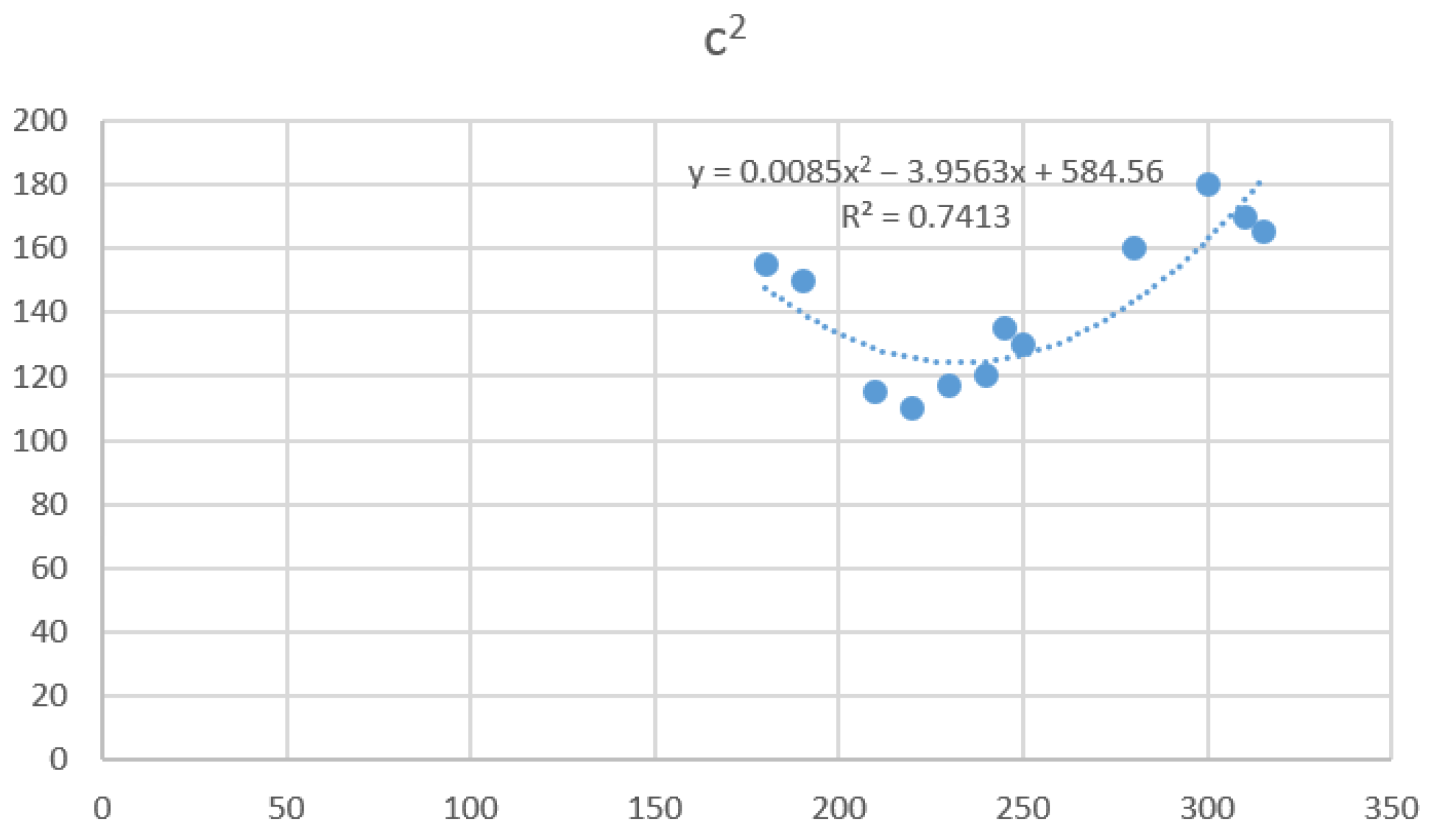
| c2 = 0.0085 (x2)2 − 3.9563 x2 + 584.56, | R2 = 0.7413, |
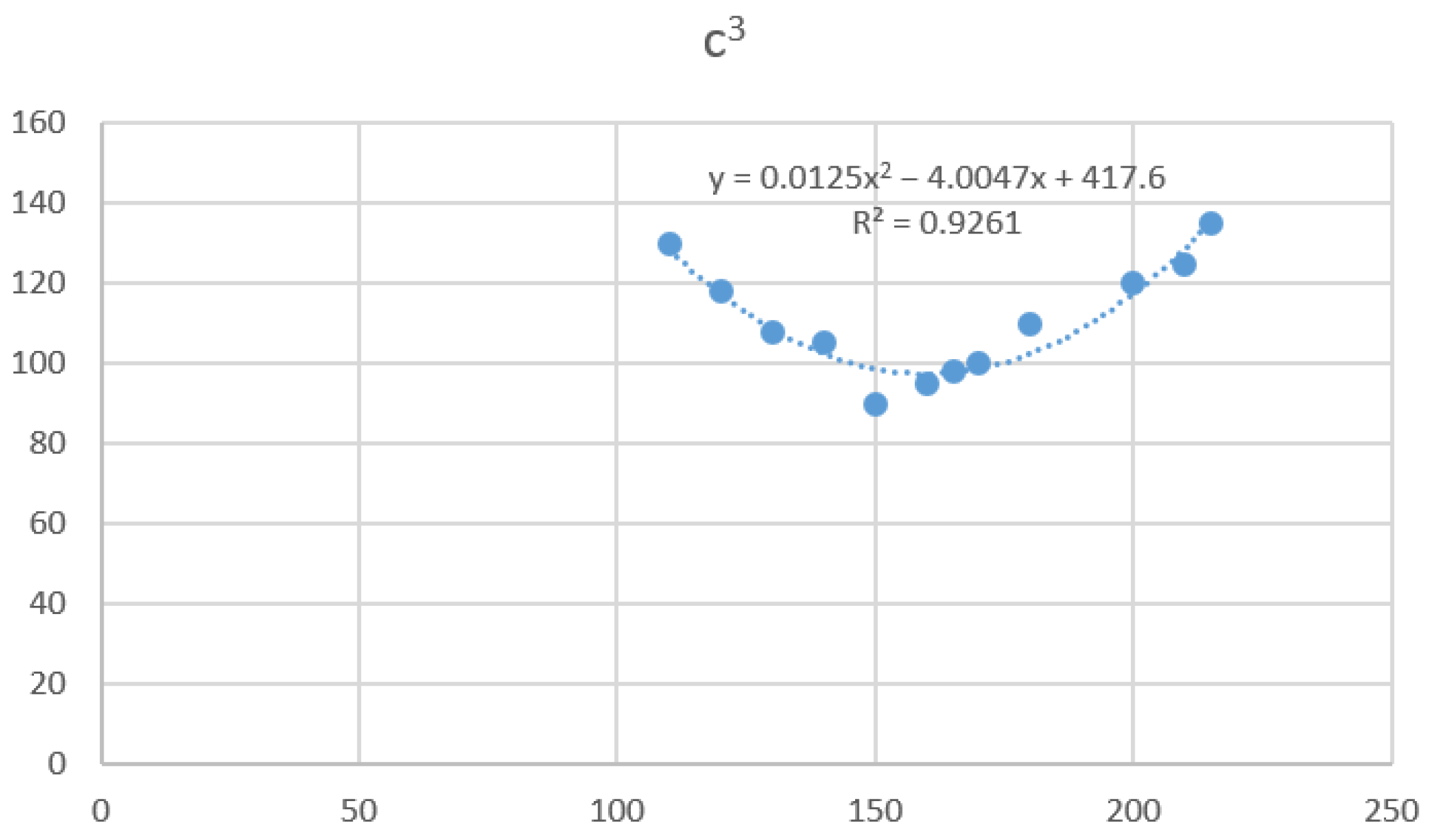
| c3 = 0.0125 (x3)2 − 4.0047 x3 + 417.6, | R2 = 0.9261, |
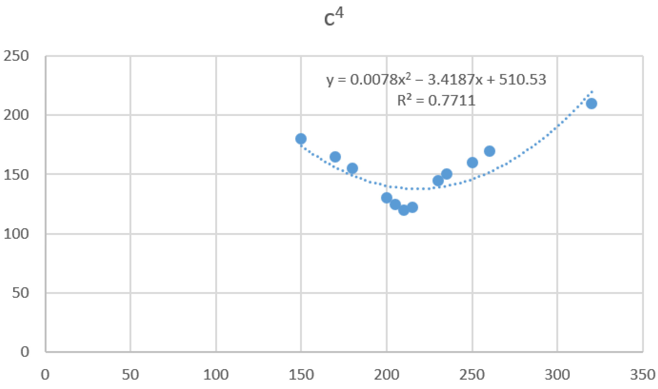
| c4 = 0.0078 (x4)2 − 3.4187 x4 + 510.53, | R2 = 0.7711. |
0.0085 (x2)2 − 3.9563 x2 + 584.56 +
0.0125 (x3)2 − 4.0047 x3 + 417.6 +
0.0078 (x4)2 − 3.4187 x4 + 510.53
x1 ≥ 0, x2 ≥ 0, x3 ≥ 0, x4 ≥ 0
4. Results and Discussion
5. Conclusions
Author Contributions
Funding
Institutional Review Board Statement
Informed Consent Statement
Data Availability Statement
Conflicts of Interest
References
- Milusheva, P. Some Aspects of the Decision to Buy, Not to Produce Parts and Components. Econ. Comput. Sci. 2019, 2, 64–67. [Google Scholar]
- Milusheva, P. Challenges to Supply Construction Companies in Conditions of Pandemic. Econ. Sci. Educ. Real Econ. Dev. Interact. Digit. Age 2020, 1, 233–237. [Google Scholar]
- Milusheva, P. Development of the Logistics in Hotels on the Bulgarian Black Sea Coast. Izv. J. Union Sci. Varna Econ. Sci. Ser. 2014, 1, 92–97. [Google Scholar]
- Milusheva, P. Aspects of the Relationships of the Companies with the Suppliers. Econ. Comput. Sci. 2016, 1, 6–10. [Google Scholar]
- Sachkov, I.N.; Marinova, O.; Turygina, V.F.; Turygin, E.E.; Dolganov, A.N. Regularities of Non-Uniform Heating of the Two-Phase Environment During Electric Current. In Proceedings of the 16th International Multidisciplinary Scientific Geoconference, Sgem 2016: Science and Technologies in Geology, Exploration and Mining, Albena, Bulgaria, 30 June–6 July 2016; Stef92 Technology Ltd.: Sofia, Bulgaria, 2016; Volume 3, pp. 599–605. [Google Scholar]
- Sachkov, I.N.; Marinova, O.; Turygina, V.F.; Turygin, E.E. The Effect of the Geometry of the Micro Pores on the Effective Permeability of Soil. In Proceedings of the International Conference on Numerical Analysis and Applied Mathematics 2015 (icnaam-2015), Rhodes, Greece, 23–29 September 2015; Simos, T., Tsitouras, C., Eds.; Amer Inst Physics: Melville, SK, Canada, 2016; Volume 1738, p. 110010. [Google Scholar]
- Balagura, K.; Kazakova, H.; Maximus, D.; Turygina, V. Mathematical Models of Cognitive Interaction Identification in the Social Networks. In Proceedings of the International Conference on Numerical Analysis and Applied Mathematics (icnaam-2018), Rhodes, Greece, 13–18 September 2018; Simos, T., Tsitouras, C., Eds.; Amer Inst Physics: Melville, SK, Canada, 2019; Volume 2116, p. 430016. [Google Scholar]
- Dolganov, A.N.; Ford, V.; Tarasyev, A.M.; Turygina, V.F. Optimiztion of Information Resources in Industrial Ecology. In Ifac Papersonline, 17th IFAC Workshop on Control Applications of Optimization CAO 2018, Yekaterinburg, Russia, 15–19 October 2018; Elsevier Science Bv: Amsterdam, The Netherlands, 2018; Volume 51, pp. 67–72. [Google Scholar]
- Tarasyev, A.M.; Turygina, V.F. Application of Material Flow Analysis in the Industry. In Proceedings of the Ecology, Economics, Education and Legislation, Albena, Bulgaria, 16–25 June 2015; Stef92 Technology Ltd.: Sofia, Bulgaria, 2015; Volume 3, pp. 71–76. [Google Scholar]
- Paraskevov, H.; Stoyanov, B. Steganographic Algorithm Based on Chaotic Random System on Raspberry Pi Hardware. In Proceedings of the Applications of Mathematics in Engineering and Economics (amee20), Sofia, Bulgaria, 7–13 June 2020; Pasheva, V., Popivanov, N., Venkov, G., Eds.; Amer Inst Physics: Melville, SK, Canada, 2021; Volume 2333, p. 70002. [Google Scholar]
- Stoyanov, B.; Ivanova, T. Pseudorandom Byte Generator Based on Shrinking 128-Bit Chaotic Function. In Proceedings of the Applications of Mathematics in Engineering and Economics (amee20), Sofia, Bulgaria, 7–13 June 2020; Pasheva, V., Popivanov, N., Venkov, G., Eds.; Amer Inst Physics: Melville, SK, Canada, 2021; Volume 2333, p. 70003. [Google Scholar]
- Todorova, M.; Stoyanov, B. Novel Hash Function Using Zaslaysky Map. In Proceedings of the Applications of Mathematics in Engineering and Economics (amee20), Sofia, Bulgaria, 7–13 June 2020; Pasheva, V., Popivanov, N., Venkov, G., Eds.; Amer Inst Physics: Melville, SK, Canada, 2021; Volume 2333, p. 70005. [Google Scholar]
- Zeng, S.; Nestorenko, O.; Nestorenko, T.; Morkūnas, M.; Volkov, A.; Baležentis, T.; Zhang, C. EOQ for Perishable Goods: Modification of Wilson’s Model for Food Retailers. Technol. Econ. Dev. Econ. 2019, 25, 1413–1432. [Google Scholar] [CrossRef] [Green Version]
- Parusheva, S.; Aleksandrova, Y.; Hadzhikolev, A. Use of Social Media in Higher Education Institutions—An Empirical Study Based on Bulgarian Learning Experience. TEM J. Technol. Educ. Manag. Inform. 2018, 7, 171–181. [Google Scholar] [CrossRef]
- Aleksandrova, Y.; Parusheva, S. Social Media Usage Patterns in Higher Education Institutions—An Empirical Study. Int. J. Emerg. Technol. Learn. 2019, 14, 108–121. [Google Scholar] [CrossRef]
- Berg, D.B.; Apanasenko, A.; Medvedeva, M.A.; Parusheva, S.S. The Entrepreneurial Network Simulation Model for the Supporting System of Management Decisions Making at a Municipal Level. In Proceedings of the International Conference on Numerical Analysis and Applied Mathematics Icnaam 2019, Rhodes, Greece, 13–18 September 2018; Simos, T., Tsitouras, C., Eds.; Amer Inst Physics: Melville, SK, Canada, 2020; Volume 2293, p. 120024. [Google Scholar]
- Miryanov, R.; Chalakova, K. One Type of Problems with Infinite Number of Cube Roots. Math. Inform. 2019, 62, 284–289. [Google Scholar]
- Miryanov, R.; Petkov, J. An Application of the Relation between Arithmetic Mean and Geometric Mean for Rational Proving Some Inequalities. Math. Inform. 2017, 60, 363–369. [Google Scholar]
- Miryanov, R.; Yordanova, V. Optimizing the Positioning of Serving Units in the Tourism Business. Math. Inform. 2017, 60, 515–520. [Google Scholar]
- Shabanova, M.; Sergeeva, T.; Nikolaev, R.; Pavlova, M. Inquiry-Based Mathematics Education in the Style of Experimental Mathematics. In Proceedings of the 12th International Technology, Education and Development Conference (inted), Valencia, Spain, 5–7 March 2018; Chova, L.G., Martinez, A.L., Torres, I.C., Eds.; Iated-Int Assoc Technology Education & Development: Valenica, Spain, 2018; pp. 7933–7941. [Google Scholar]
- Grozdev, S.; Nikolaev, R.; Nenkov, V. National Mathematical Olympiad for University Students. Math. Inform. 2017, 60, 291–294. [Google Scholar]
- Nacheva, R.; Jansone, A. Multi-Layered Higher Education E-Learning Framework. Balt. J. Mod. Comput. 2021, 9, 345–362. [Google Scholar] [CrossRef]
- Nacheva, R.; Jansone, A. Current Perspectives in Social Media Supported E-Learning. Balt. J. Mod. Comput. 2022, 10, 71–86. [Google Scholar] [CrossRef]
- Polkowski, Z.; Nycz-Lukaszewska, M. Infrastructure as a Service: Cloud Computing Model for Micro Companies. In Proceedings of the Advances in Data Science and Management, Singapore, 14 January 2020; Borah, S., Balas, V.E., Polkowski, Z., Eds.; Springer-Verlag Singapore Pte Ltd.: Singapore, 2020; Volume 37, pp. 307–320. [Google Scholar]
- Polkowski, Z.; Prakash Mishra, J.; Sourav Prasad, S.; Kumar Mishra, S. Evaluation of Aggregated Query Plans Using Heuristic Approach. In Proceedings of the Proceedings of the 2020 12th International Conference on Electronics, Computers and Artificial Intelligence (ecai-2020), Bucharest, Romania, 25–27 June 2020; IEEE: New York, NY, USA, 2020. [Google Scholar]
- Polkowski, Z.; Vora, J.; Tanwar, S.; Tyagi, S.; Singh, P.K.; Singh, Y. Machine Learning-Based Software Effort Estimation: An Analysis. In Proceedings of the 11th International Conference on Electronics, Computers and Artificial Intelligence (ecai-2019), Arges, Romania, 27–29 June 2019; IEEE: New York, NY, USA, 2019. [Google Scholar]
- Prakash Mishra, J.; Polkowski, Z.; Kumar Mishra, S. Performance of Cloudlets in Task Implementation Using Ant Colony Optimization Technique. In Proceedings of the 2020 12th International Conference on Electronics, Computers and Artificial Intelligence (ecai-2020), Bucharest, Romania, 25–27 June 2020; IEEE: New York, NY, USA, 2020. [Google Scholar]
- Nacheva, R.; Jansone, A. Usability Evaluation of Business Process Modelling Tools through Software Quality Metrics. Balt. J. Mod. Comput. 2020, 8, 534–542. [Google Scholar] [CrossRef]
- Petrov, P.; Krumovich, S.; Nikolov, N.; Dimitrov, G.; Sulov, V. Web Technologies Used in the Commercial Banks in Finland. In Proceedings of the Computer Systems and Technologies (compsystech’18), Ruse, Bulgaria, 13–14 September 2018; Rachev, B., Smrikarov, A., Eds.; Assoc Computing Machinery: New York, NY, USA, 2018; Volume 1641, pp. 94–98. [Google Scholar]
- Sulov, V. Iteration vs Recursion in Introduction to Programming Classes: An Empirical Study. Cybern. Inf. Technol. 2016, 16, 63–72. [Google Scholar] [CrossRef] [Green Version]
- Kuyumdzhiev, I.O. Controls Mitigating the Risk of Confidential Information Disclosure by Facebook: Essential Concern in Auditing Information Security. TEM J. Technol. Educ. Manag. Inform. 2014, 3, 113–119. [Google Scholar]
- Sulova, S. Models for Web Applications Data Analysis. In Proceedings of the Computer Systems and Technologies, Ruse, Bulgaria, 21–22 June 2019; Vassilev, T., Smrikarov, A., Eds.; Assoc Computing Machinery: New York, NY, USA, 2019; pp. 246–250. [Google Scholar]
- Sulova, S. Association Rule Mining for Improvement of IT Project Management. TEM J. Technol. Educ. Manag. Inform. 2018, 7, 717–722. [Google Scholar] [CrossRef]
- Nacheva, R.; Sulov, V.; Czaplewski, M. The Impact of M-Learning on Sustainable Information Society. In Proceedings of the International Conference on Electronic Governance and Open Society: Challenges in Eurasia, Saint Petersburg, Russia, 24–25 November 2021; Springer: Berlin/Heidelberg, Germany, 2022; pp. 244–262. [Google Scholar]
- Nacheva, R. Digital Inclusion Through Sustainable Web Accessibility. In Proceedings of the Digital Transformation and Global Society, Dtgs 2021, Petersburg, Russia, 23–25 June 2021; Alexandrov, D.A., Boukhanovsky, A.V., Chugunov, A.V., Kabanov, Y., Koltsova, O., Musabirov, I., Pashakhin, S., Eds.; Springer International Publishing Ag: Cham, Switzerland, 2022; Volume 1503, pp. 83–96. [Google Scholar]
- Aleksandrova, Y. Comparing Performance of Machine Learning Algorithms for Default Risk Prediction in Peer to Peer Lending. TEM J. Technol. Educ. Manag. Inform. 2021, 10, 133–143. [Google Scholar] [CrossRef]
- Stoyanova, M. Good Practices and Recommendations for Success in Construction Digitalization. TEM J. Technol. Educ. Manag. Inform. 2020, 9, 42–47. [Google Scholar] [CrossRef]
- Petrov, P.; Radev, M.; Dimitrov, G.; Simeonidis, D. Infrastructure Capacity Planning in Digitalization of Educational Services. Int. J. Emerg. Technol. Learn. 2022, 17, 299–306. [Google Scholar] [CrossRef]
- Petrov, P.; Radev, M.; Dimitrov, G.; Pasat, A.; Buevich, A. A Systematic Design Approach in Building Digitalization Services Supporting Infrastructure. TEM J. Technol. Educ. Manag. Inform. 2021, 10, 31–37. [Google Scholar] [CrossRef]
- Ropi, N.M.; Hishamuddin, H.; Wahab, D.A.; Saibani, N. Optimisation Models of Remanufacturing Uncertainties in Closed-Loop Supply Chains–A Review. IEEE Access 2021, 9, 160533–160551. [Google Scholar] [CrossRef]
- Optimisation Models and Information Sharing in a Multi-Echelon Pharmaceutical Supply Chain|International Journal of Shipping and Transport Logistics. Available online: https://www.inderscienceonline.com/doi/abs/10.1504/IJSTL.2022.120670 (accessed on 20 July 2022).
- Becerra, P.; Mula, J.; Sanchis, R. Green Supply Chain Quantitative Models for Sustainable Inventory Management: A Review. J. Clean. Prod. 2021, 328, 129544. [Google Scholar] [CrossRef]
- Kulkarni, P.; Azizi, V.; Wang, L.; Hu, G. Analysis of Decision Making and Information Sharing Strategies in a Two-Echelon Supply Chain. Int. J. Supply Chain Inventory Manag. 2021, 4, 81–106. [Google Scholar] [CrossRef]
- Krzyżaniak, S. Optimisation of the Stock Structure of a Single Stock Item Taking into Account Stock Quantity Constraints, Using a Lagrange Multiplier. Logforum 2022, 18, 261–269. [Google Scholar] [CrossRef]
- Faramarzi-Oghani, S.; Dolati Neghabadi, P.; Talbi, E.-G.; Tavakkoli-Moghaddam, R. Meta-Heuristics for Sustainable Supply Chain Management: A Review. Int. J. Prod. Res. 2022, 1–31. [Google Scholar] [CrossRef]
- El Jaouhari, A.; Alhilali, Z.; Arif, J.; Fellaki, S.; Amejwal, M.; Azzouz, K. Demand Forecasting Application with Regression and IoT Based Inventory Management System: A Case Study of a Semiconductor Manufacturing Company. Int. J. Eng. Res. Afr. 2022, 60, 189–210. [Google Scholar] [CrossRef]
- Finco, S.; Battini, D.; Converso, G.; Murino, T. Applying the Zero-Inflated Poisson Regression in the Inventory Management of Irregular Demand Items. J. Ind. Prod. Eng. 2022, 1–21. [Google Scholar] [CrossRef]
- Kim, G. A Study on Determinants of Inventory Turnover Using Quantile Regression Analysis. Asia Pac. J. Bus. 2022, 13, 185–195. [Google Scholar] [CrossRef]
- Kovtun, N.; Yushchenko, N. Logistics Models of Modernization of Distribution and Transmission Systems for the Development of Ukraine as an Exporter of Green Energy. In Proceedings of the MATEC Web of Conferences; EDP Sciences, Cape Town, South Africa, 29 November–1 December 2021. [Google Scholar]
- Yamsaard, S. Managing International Perishable Food Supply Chain: A Literature Review. In Proceedings of the 2021 1st International Conference on Cyber Management and Engineering (CyMaEn), Virtual, 26–28 May 2021; IEEE: New York, NY, USA, 2021; pp. 1–6. [Google Scholar]
- Shah, N.H.; Patel, E.; Rabari, K. Investigation of Carbon Emissions Due to COVID-19 Vaccine Inventory. Int. J. Syst. Assur. Eng. Manag. 2022, 13, 409–420. [Google Scholar] [CrossRef]
- Galkin, A.; Yemchenko, I.; Lysa, S.; Tarasiuk, M.; Chortok, Y.; Khvesyk, Y. EXPLORING THE RELATIONSHIPS BETWEEN DEMAND ATTITUDES AND THE SUPPLY AMOUNT IN CONSUMER-DRIVEN SUPPLY CHAIN FOR FMCG. Acta Logist. 2022, 9, 1–12. [Google Scholar] [CrossRef]
- Istiningrum, A.A.; Sono, S.; Putri, V.A. Inventory Cost Reduction and EOQ for Personal Protective Equipment: A Case Study in Oil and Gas Company. J. Logist. Indones. 2021, 5, 86–103. [Google Scholar] [CrossRef]
- POPOVA, I.N.; VLASOV, A.I.; NIKITINA, N.I. Optimization of Inventory Distribution Logistics in Industrial Enterprises. Rev. Espac. 2018, 39, 16–24. [Google Scholar]
- Cristescu, M.P.; Flori, M.; Nerisanu, R.A. Applying a Sustainable Vector Model to Generate Innovation. In Education, Research and Business Technologies; Springer: Berlin/Heidelberg, Germany, 2022; pp. 149–161. [Google Scholar]
- Dogaru, V.; Brandas, C.; Cristescu, M. An Urban System Optimization Model Based on CO2 Sequestration Index: A Big Data Analytics Approach. Sustainability 2019, 11, 4821. [Google Scholar] [CrossRef] [Green Version]
- Trifonova, E.; Valchev, N.; Keremedchiev, S.; Kotsev, I.; Eftimova, P.; Todorova, V.; Konsulova, T.; Doncheva, V.; Flipova-Marinova, M.; Vergiev, S.; et al. Case Studies Worldwide: Mitigating Flood and Erosion Risk Using Sediment Management for a Tourist City: Varna, Bulgaria. In Coastal Risk Management in a Changing Climate; Elsevier: Amsterdam, The Netherlands, 2014; pp. 358–383. ISBN 978-0-12-397331-3. [Google Scholar]
- Grozdev, S.; Nikolaev, R.; Stoilova, S.; Nenkov, V. 45th National Olympiad in Mathematics for University Students. Math. Inform. 2018, 61, 294–298. [Google Scholar]
- Nikolaev, R.; Grozdev, S.; Patronova, N.; Koneva, B.; Shabanova, M. Bulgarian Olympiad on Financial and Actuarial Mathematics in Russia. Math. Inform. 2019, 62, 676–694. [Google Scholar]
- Grozdev, S.; Nikolaev, R.; Patronova, N.; Forkunova, L.; Shabanova, M. Results of the Second International Olympiad in Financial and Actuarial Mathematics for School and University Students. Math. Inform. 2018, 61, 423–443. [Google Scholar]


| j i | x1 | x2 | … | xj | … | xn |
|---|---|---|---|---|---|---|
| 1 | x11 | x12 | … | x1j | … | x1n |
| 2 | x21 | x22 | … | x2j | … | x2n |
| … | … | … | … | … | … | … |
| i | xi1 | xi2 | … | xij | … | xin |
| … | … | … | … | … | … | … |
| m | xm1 | xm2 | … | xmj | … | xmn |
| j i | c1 | c2 | … | cj | … | cn |
|---|---|---|---|---|---|---|
| 1 | c11 | c12 | … | c1j | … | c1n |
| 2 | c21 | c22 | … | c2j | … | c2n |
| … | … | … | … | … | … | … |
| i | ci1 | ci2 | … | cij | … | cin |
| … | … | … | … | … | … | … |
| m | cm1 | cm2 | … | cmj | … | cmn |
| Product | A1 | A2 | A3 | A4 |
|---|---|---|---|---|
| xi Month | x1 | x2 | x3 | x4 |
| 1 | 200 | 300 | 180 | 250 |
| 2 | 120 | 220 | 210 | 230 |
| 3 | 180 | 250 | 160 | 235 |
| 4 | 130 | 240 | 140 | 260 |
| 5 | 240 | 190 | 110 | 320 |
| 6 | 260 | 210 | 150 | 180 |
| 7 | 210 | 280 | 170 | 200 |
| 8 | 150 | 310 | 200 | 210 |
| 9 | 110 | 245 | 215 | 170 |
| 10 | 165 | 315 | 165 | 150 |
| 11 | 170 | 230 | 130 | 205 |
| 12 | 160 | 180 | 120 | 215 |
| Costs Month | c1 | c2 | c3 | c4 |
|---|---|---|---|---|
| 1 | 130 | 180 | 110 | 160 |
| 2 | 140 | 110 | 125 | 145 |
| 3 | 100 | 130 | 95 | 150 |
| 4 | 125 | 120 | 105 | 170 |
| 5 | 170 | 150 | 130 | 210 |
| 6 | 180 | 115 | 90 | 155 |
| 7 | 135 | 160 | 100 | 130 |
| 8 | 130 | 170 | 120 | 120 |
| 9 | 120 | 135 | 135 | 165 |
| 10 | 110 | 165 | 98 | 180 |
| 11 | 105 | 117 | 108 | 125 |
| 12 | 115 | 155 | 118 | 122 |
| A1 | A2 | A3 | A4 | ||||
|---|---|---|---|---|---|---|---|
| x1 | c1 | x2 | c2 | x3 | c3 | x4 | c4 |
| 110 | 120 | 180 | 155 | 110 | 130 | 150 | 180 |
| 120 | 140 | 190 | 150 | 120 | 118 | 170 | 165 |
| 130 | 125 | 210 | 115 | 130 | 108 | 180 | 155 |
| 150 | 130 | 220 | 110 | 140 | 105 | 200 | 130 |
| 160 | 115 | 230 | 117 | 150 | 90 | 205 | 125 |
| 165 | 110 | 240 | 120 | 160 | 95 | 210 | 120 |
| 170 | 105 | 245 | 135 | 165 | 98 | 215 | 122 |
| 180 | 100 | 250 | 130 | 170 | 100 | 230 | 145 |
| 200 | 130 | 280 | 160 | 180 | 110 | 235 | 150 |
| 210 | 135 | 300 | 180 | 200 | 120 | 250 | 160 |
| 240 | 170 | 310 | 170 | 210 | 125 | 260 | 170 |
| 260 | 180 | 315 | 165 | 215 | 135 | 320 | 210 |
Publisher’s Note: MDPI stays neutral with regard to jurisdictional claims in published maps and institutional affiliations. |
© 2022 by the authors. Licensee MDPI, Basel, Switzerland. This article is an open access article distributed under the terms and conditions of the Creative Commons Attribution (CC BY) license (https://creativecommons.org/licenses/by/4.0/).
Share and Cite
Vasilev, J.; Milkova, T. Optimisation Models for Inventory Management with Limited Number of Stock Items. Logistics 2022, 6, 54. https://doi.org/10.3390/logistics6030054
Vasilev J, Milkova T. Optimisation Models for Inventory Management with Limited Number of Stock Items. Logistics. 2022; 6(3):54. https://doi.org/10.3390/logistics6030054
Chicago/Turabian StyleVasilev, Julian, and Tanka Milkova. 2022. "Optimisation Models for Inventory Management with Limited Number of Stock Items" Logistics 6, no. 3: 54. https://doi.org/10.3390/logistics6030054