Composing Vessel Fleets for Maintenance at Offshore Wind Farms by Solving a Dual-Level Stochastic Programming Problem Using GRASP

Abstract

Background: Dual-level stochastic programming is a technique that allows modelling uncertainty at two different levels, even when the time granularity differs vastly between the levels. In this paper we study the problem of determining the optimal fleet size and mix of vessels performing maintenance operations at offshore wind farms. In this problem the strategic planning spans decades, while operational planning is performed on a day-to-day basis. Since the operational planning level must somehow be taken into account when making strategic plans, and since uncertainty is present at both levels, dual-level stochastic programming is suitable. Methods: We present a heuristic solution method for the problem based on the greedy randomized adaptive search procedure (GRASP). To evaluate the operational costs of a given fleet, a novel fleet deployment heuristic (FDH) is embedded into the GRASP. Results: Computational experiments show that the FDH produces near optimal solutions to the operational day-to-day fleet deployment problem. Comparing the GRASP to exact methods, it produces near optimal solutions for small instances, while significantly improving the primal solutions for larger instances, where the exact methods do not converge. Conclusions: The proposed heuristic is suitable for solving realistic instances, and produces near optimal solution in less than 2 h.

1. Introduction

This work is motivated by solving a maritime fleet size and mix problem (MFSMP) arising when planning the maintenance of turbines in offshore wind farms. Maintenance tasks must be performed both to reduce the risk of turbine failures and to repair turbines following a breakdown. The particular MFSMP studied was presented by Stålhane et al. [1], who referred to it as the dual-level fleet size and mix problem for conducting maintenance at offshore wind farms (DLPOW). The problem involves strategic decisions regarding the fleet size and mix, spanning the lifetime of a wind farm. However, to evaluate fleet composition decisions, one must also consider operational decisions, which are made on a day-to-day basis, regarding which maintenance tasks to perform, and which vessels to use to support each maintenance task.

As both strategic and operational decisions are influenced by uncertainty, the DLPOW was modelled as a dual-level stochastic problem. In particular, there is long-term uncertainty influencing the future electricity prices and the completion of different parts of the wind farm, which is captured in a multi-stage scenario tree. At the same time, there is short-term uncertainty in the number of maintenance tasks required, and the weather conditions at the wind farms that affects a vessel’s ability to operate, which is captured in additional operational scenarios connected to each node of the strategic scenario tree.

Stålhane et al. [1] solved the DLPOW using a commercial mixed-integer programming (MIP) solver and an ad hoc solution method based on the integer L-shaped method [2]. Only small instances could be tackled by the direct formulation, while the integer L-shaped could solve slightly larger instances. The authors therefore suggested the design of efficient heuristic solution methods as future work. However, there is little past research on how to design heuristics for similar problems.

Until the paper of Stålhane et al. [1], the only paper published on MFSMPs for supporting maintenance activities at offshore wind farms that included long-term uncertainty is that of Gundegjerde et al. [3]. They proposed a three-stage stochastic program that considered uncertainty in vessel spot rates, electricity prices, weather conditions, and the failure rates of wind turbines. However, only short-term uncertainty was considered during the operational life of the wind farm, while the sources of long-term uncertainty (electricity prices and vessel charter rates) were only considered between the time of commissioning and the start of operation of the wind farm. Other studies have all presented two-stage stochastic programs where only short-term uncertainty was considered [4,5,6,7].

Gundegjerde et al. [3] and Stålhane et al. [4] solved the deterministic equivalent of their stochastic programs using commercial solvers, while Stålhane et al. [6] and Gutierrez-Alcoba et al. [7] presented matheuristics for the problem. Both matheuristics rely on a Dantzig-Wolfe reformulation of the deterministic equivalent, where potential daily work schedules for the vessel types are generated heuristically, and a master problem is used to select a subset of these work schedules for each day in each scenario, for a given fleet. Halvorsen-Weare et al. [5] presented a greedy randomized adaptive search procedure (GRASP) where the fleet is built by successively adding vessels, and each fleet is evaluated using a simulation model. However, they considered only one decision stage where vessels can be chartered in and out, and thus did not consider different charter lengths, nor changes to the wind farm over time.

Pantuso et al. [8] pointed out that little research has been published on MFSMPs dealing with uncertainty. In relation to this, most work on fleet composition for offshore supply vessels in the oil industry consider deterministic problems, with a recent example from Vieira et al. [9]. However, Pantuso et al. [10] considered a dual-level stochastic MFSMP and presented a heuristic solution method. They distinguished between two types of decisions: aggregate-level decisions and detailed-level decisions, both of which are subject to uncertainty. The resulting stochastic program had block-separable recourse [11]. This property was exploited to decompose the problem into a master problem and many independent linear programming subproblems. The master problem was solved by a tabu search heuristic, while the subproblems were solved to optimality. Results indicated that the heuristic solution procedure was less efficient than directly using a commercial solver for small instances, but significantly better for larger problem instances.

For the DLPOW, however, the subproblems are not simple LPs. Furthermore, the master problem still has a scenario tree structure, which is likely to be unfavorable for local search-based metaheuristics, such as tabu search: making small adjustments to the fleet composition at any node of the scenario tree potentially influences the decisions at all other nodes of the tree.

Hvattum et al. [12] applied a GRASP to a scenario-tree-based formulation of a stochastic inventory-routing problem. Only the construction phase of GRASP was included, while the local search phase was omitted. In a computational study, the performance of the GRASP was benchmarked against an exact solution method and several simple matheuristics. The results were favorable for the GRASP.

In summary, the scientific literature has not thoroughly presented and evaluated the application of metaheuristics to deal with dual-level stochastic optimization problems. In this paper, a reactive GRASP [13] is implemented for the DLPOW, exploiting ideas from Hvattum et al. [12] and Pantuso et al. [10]. This appears to be only the second application of a GRASP to any stochastic programming problem [12,14,15]. At the same time, it may be the first time that GRASP has been used to solve any MFSMP [1,8], and only the second application of any metaheuristic to a dual-level stochastic problem [10,16]. The surveys of metaheuristics for stochastic problems by Bianchi et al. [17], Gutjahr [18], and Hvattum and Esbensen [19] provide further evidence that GRASP has very rarely been used to solve problems with uncertainty. On the other hand, other metaheuristics have been tested in settings with uncertainty recently, such as genetic algorithms, particle swarm optimization, and bee colony algorithms [20]; tabu search [21]; differential evolution [22]; and invasive weed optimization [23].

The remainder of this paper is structured as follows. Section 2 describes the DLPOW. The GRASP implemented to solve the DLPOW is explained in Section 3. An extensive computational study is summarized in Section 4, followed by concluding remarks in Section 5.

2. Problem Description and Mathematical Model

The problem studied in this paper is designed to capture the situation of future large-scale wind farm projects, which are developed in several steps. One example is the Dogger Bank project outside of the UK, which will be developed in three steps referred to as Dogger Bank A, B, and C, each with an installed capacity of 1.2 GW [24]. Other examples are the Empire Wind and the Beacon Wind projects off the US East Coast, which will each be developed in two steps [25]. Most new tenders for offshore wind farms are now won without subsidies, with 2.5 GW of zero-subsidy capacity already bid into the European offshore markets [26]. A lack of subsidies leads to more uncertainty related to the future value of the electricity generated at the wind farms, making it more important for the operators to consider long-term changes in the electricity price in the maintenance planning as well.

In the following, we first give a short description of the problem in Section 2.1, before explaining the structure of a dual-level scenario tree in the context of the DLPOW in Section 2.2. Finally, we present a mathematical model of the DLPOW in Section 2.3.

2.1. Problem Description

The DLPOW consists in determining the optimal fleet size and mix of vessels to support maintenance activities at one or more offshore wind farms. Given that these wind farms are relatively close to each other, it is likely that substantial savings can be made by having a common vessel fleet supporting their joint maintenance needs. Since the wind farms may have a step-wise development, it is important to look at the total life-span of the farms, as the number of maintenance operations are expected to vary over time.

We consider a wind farm operator employing a maintenance strategy combining periodic and condition-based maintenance. This entails that each turbine is subject to a major overhaul at regular time intervals, while additional maintenance is performed to replace components that have broken down. Once a component is broken, the turbine is shut down, and the operator loses revenue until the turbine is operational again. This loss of revenue is commonly referred to as downtime cost, and depends on the longevity of the shutdown, the electricity price, and the wind conditions during the shut down. Downtime costs also occur during the periodic maintenance activities, since the turbine has to be shut down during the maintenance.

Each maintenance task requires a number of technicians for a given number of hours, and it is assumed that the maintenance can be conducted over several days. The technicians are transported to and from the wind farms using special-purpose vessels. The vessels are restricted with respect to how many technicians they may carry and what weather conditions they can operate in, and the vessels may be chartered on long-term or short-term contracts. The short-term charter contracts have durations varying from a month up to one year, while long-term charter contracts may last a number of years, potentially spanning the entire lifetime of the vessel. It is typically less expensive to charter a vessel for a longer period, but short-term charters may be convenient to cover peaks in the maintenance demands, for example in periods where major overhauls of the turbines are planned.

The vessels operate from a maintenance base, which traditionally has been located at a harbour along the coast, close to the wind farms. However, as the wind farms are moving further offshore, several advanced concepts, such as maintenance platforms and artificial maintenance islands, have also been proposed. Given that the choice of maintenance base has a huge influence on the operations, it must also be considered when choosing a vessel fleet at a strategic level.

The problem is subject to uncertainty both at a strategic and an operational level. On the strategic level, there is uncertainty regarding when, and if, the planned wind farm projects are developed. Often these projects are developed in steps, and delays may occur in this development. In addition, long-term changes in the electricity price, for example caused by changes to the subsidy schemes, will affect the downtime costs. On the operational level, there is uncertainty in the number of condition-based maintenance tasks to perform and in the weather conditions in which the vessels must support the maintenance tasks.

2.2. Dual-Level Scenario Trees Applied to the DLPOW

Since decisions must be made at both the strategic and operational levels, the time horizon is divided into stages, and in each stage strategic decisions must be made regarding the fleet composition. Once the fleet size and mix has been decided for a given stage, the vessels are used to support maintenance tasks in the time period until the next stage. Once the next stage is reached, some of the uncertain strategic parameters are revealed.

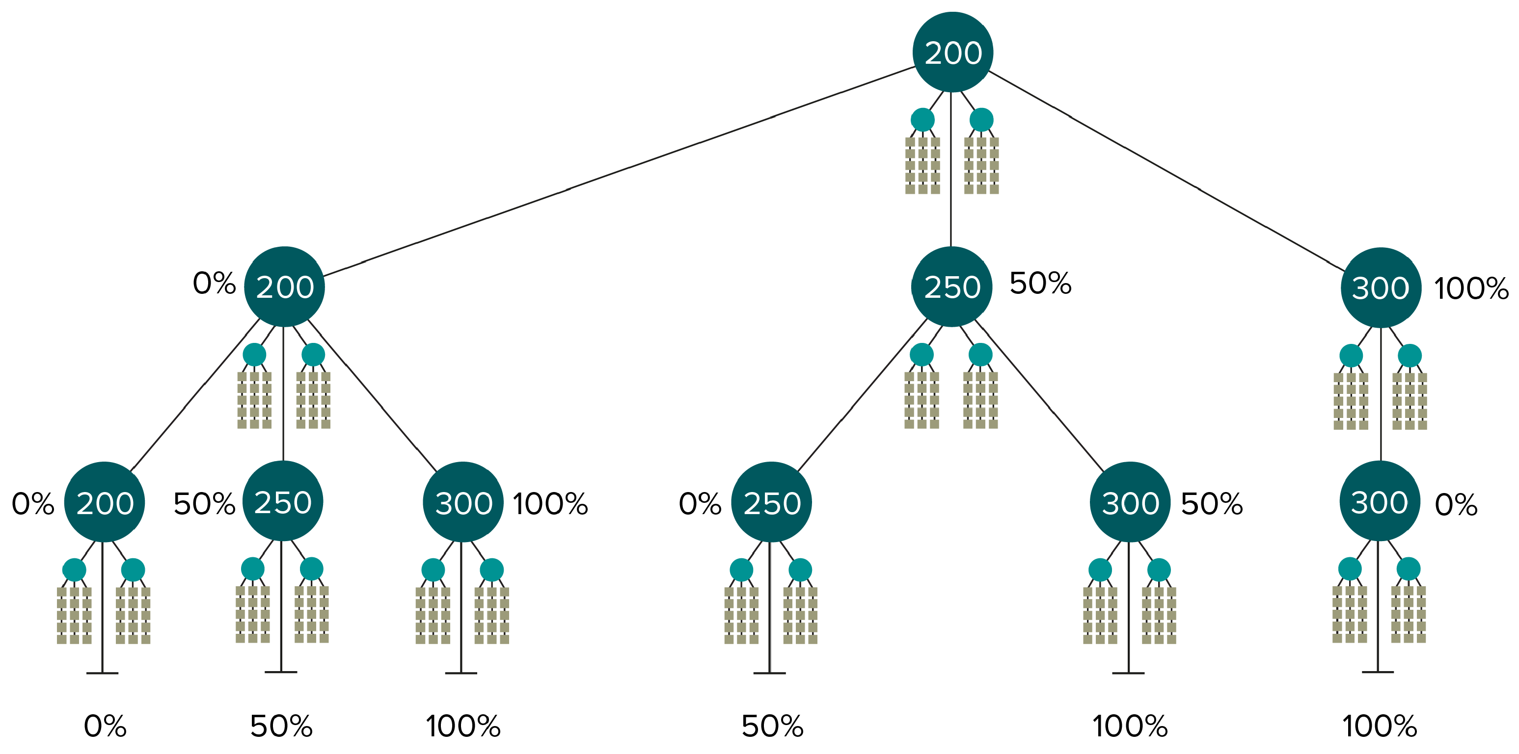
Figure 1 shows a scenario tree where there is uncertainty in the step-wise wind farm development. The wind farm initially consists of 200 turbines, as indicated by the root node of the tree. The plan is that 100 additional turbines are realized in year 10, corresponding to the second level of the tree (stage 2). However, the installation of these turbines is uncertain, and the numbers given inside the large circles representing each strategic node indicate the total number of turbines actually installed at the wind farm at the respective nodes. The percentage next to each strategic node gives the percentage of the 100 planned turbines that has been installed at that strategic node.

Below each strategic node, there are two smaller nodes, corresponding to the winter season and summer season, respectively. While the period between successive strategic stages may last several years, it is assumed that the characteristics of each winter season and each summer season are the same. Thus, these are all joined under the two different season types. One reason for including different seasons is that different vessel fleets may be suitable for different seasons, partly because weather conditions may influence which vessels can be used, and partly because the demand for maintenance may differ. Thus, short-term charters are allowed to vary based on season types. While the season type is not the outcome of a random event, there is a specific portion of the total time during a year which falls into each season, and the costs pertaining to each season type can be weighted accordingly to determine an expected cost overall.

For each strategic node, and each season type associated to that node, there is then a set of operational scenarios reflecting the maintenance needs that may appear in the corresponding season. These scenarios are short, spanning only a modest number of days, but are essential to estimate the cost of using the obtained fleet to support the required maintenance tasks. Given that the important output of the model is the strategic decisions, the operational scenarios are not themselves modelled as multi-stage problems, but rather as a scenario cluster.

2.3. Mathematical Model

First, a node-based formulation for the deterministic equivalent of the multi-stage stochastic programming problem representing the strategic decisions is given. This formulation encapsulates the corresponding two-stage problems representing the operational decisions within each strategic node by defining a subproblem for each operational scenario that is a function of the available vessel fleet. Second, the subproblem for the operational planning is provided.

2.3.1. Strategic Model

For a strategic node n, the quantity $x_{vnl}$ identifies the number of vessels of type v that are chartered on a contract with expiration time l. Additional vessels can be obtained on short-term charter. For strategic node n in season type q, $y_{nqv}^{IN}$ is the number of vessels of type v that is chartered in for season type q. There is also the possibility of chartering out vessels for a given season type, and $y_{nqv}^{OUT}$ denotes the number of vessels of type v chartered out for season type q at node n.

Each operational scenario s from season type q at node n contains a number of periods p. In each period, each vessel in the fleet is deployed to a given wind farm f, where it transports technicians to, from, and between wind turbines, so that they can perform maintenance tasks. It is assumed that the operational costs of the vessels are directly proportional to the number of hours they are used in a given time period, and that this number varies between vessel types.

For the strategic level of the model, we need the following notation. The set of potential bases from where the O&M operations are staged (harbors and offshore stations) is denoted by D. The total cost of building and operating base d is $C_d^D$, and it has a maximum capacity of $M_d^D$ vessels. The set of vessel types is V, and a vessel of type v is considered to take up a capacity of $G_{vd}$ when located at base d. The choice of which bases to operate is made at the first decision stage.

Let N represent the set of strategic nodes, let $A_n$ be the set of all ancestor nodes for node n, and let $a\left(n\right)$ be the direct parent node of n. The number of years between each stage can vary, but all strategic nodes appearing at the same stage of the scenario tree correspond to the same year. Let $t\left(n\right)$ denote the year of node n. The number of years separating the strategic nodes a and b is hence $t\left(b\right)-t\left(a\right)$. Each leaf node of the scenario tree has a duration of one year. The probability of node n occurring is $B_n^S$, and the node has a discount factor of $Z_n$.

There is a fixed cost $C_{nv}^F$ for operating a vessel of type v in node n, and a charter cost $C_{nvl}^{TC}$ of chartering a vessel of type v on a long-term charter in node n with lease expiration l. The set of possible lease expiration times for a vessel of type v being chartered in node n is $L_{nv}$. Lease expiration times represent the year of the planning horizon where the vessel lease expires, and a chartered vessel will be removed from the fleet at the beginning of this year.

The set of season types Q contains two seasons q, representing summer and winter, respectively. The cost of chartering in an additional vessel of type v for a single season type q in node n is $C_{nqv}^{ST}$, while the revenue for chartering out a corresponding vessel is $R_{nqv}$. To capture the short-term operational uncertainty of a given season type q in strategic node n, we use a set of scenarios $S_{nq}$ with corresponding probabilities $B_{nqs}^T$.

In addition to the decision variables already mentioned, we define the binary variable ${\delta }_d$ to equal one if base d is used and zero otherwise. Auxiliary variables $w_{nv}$ represent the number of long-term chartered vessels of type v in node n, and $z_{nqv}$ represents the number of vessels of type v available in season type q at node n. Finally, the recourse function ${\Omega }_{nqs}\left(z_{nq}\right)$ represents the operational costs and downtime costs of using fleet $z_{nq}={\left\{z_{nqv}\right\}}_{v\in V}$ in scenario s in season type q at node n. This gives the following model:

$$\begin{array}{cc}\hfill \min z=& \sum _{n\in N}\sum _{v\in V}\frac{B_n^S}{Z_n}\left(\sum _{l\in L_{nv}}{C}_{nvl}^{TC}{x}_{nvl}+C_{nv}^F{w}_{nv}+\sum _{q\in Q}(C_{nqv}^{ST}{y}_{nqv}^{IN}-R_{nqv}{y}_{nqv}^{OUT})\right)\hfill \\ \hfill & +\sum _{d\in D}{C}_d^D{\delta }_d+\sum _{n\in N}\sum _{q\in Q}\sum _{s\in S_{nq}}\frac{B_{nqs}^T}{Z_n}{\Omega }_{nqs}\left(z_{nq}\right),\hfill \end{array}$$

(1)

$$\begin{array}{cccc}\hfill & \sum _{l\in L_{nv}}{x}_{nvl}+w_{a\left(n\right)v}-\sum _{n^{{}^{\prime }}\in A_n}{x}_{n^{{}^{\prime }}vt\left(n\right)}=w_{nv},\hfill & \hfill & n\in N\backslash \left\{1\right\},v\in V,\hfill \end{array}$$

(2)

$$\begin{array}{cccc}\hfill & \sum _{l\in L_{nv}}{x}_{nvl}=w_{nv},\hfill & \hfill & n=1,v\in V,\hfill \end{array}$$

(3)

$$\begin{array}{cccc}\hfill & y_{nqv}^{OUT}\le w_{nv},\hfill & \hfill & n\in N,q\in Q,v\in V,\hfill \end{array}$$

(4)

$$\begin{array}{cccc}\hfill & \sum _{v\in V_d}{G}_{vd}(w_{nv}+y_{nqv}^{IN})\le M_d^D{\delta }_d,\hfill & \hfill & n\in N,q\in Q,d\in D,\hfill \end{array}$$

(5)

$$\begin{array}{cccc}\hfill & w_{vn}+y_{nqv}^{IN}-y_{nqv}^{OUT}=z_{nqv},\hfill & \hfill & n\in N,q\in Q,v\in V,\hfill \end{array}$$

(6)

$$\begin{array}{cccc}\hfill & x_{nvl}\ge 0\mathrm{and}\mathrm{integer},\hfill & \hfill & n\in N,v\in V,l\in L_{nv},\hfill \end{array}$$

(7)

$$\begin{array}{cccc}\hfill & w_{nv}\ge 0\mathrm{and}\mathrm{integer},\hfill & \hfill & n\in N,v\in V,\hfill \end{array}$$

(8)

$$\begin{array}{cccc}\hfill & z_{nqv}\ge 0\mathrm{and}\mathrm{integer},\hfill & \hfill & n\in N,q\in Q,v\in V,\hfill \end{array}$$

(9)

$$\begin{array}{cccc}\hfill & y_{nqv}^{IN}\ge 0\mathrm{and}\mathrm{integer},\hfill & \hfill & n\in N,q\in Q,v\in V|L_{nv}\ne \varnothing ,\hfill \end{array}$$

(10)

$$\begin{array}{cccc}\hfill & y_{nqv}^{OUT}\ge 0\mathrm{and}\mathrm{integer},\hfill & \hfill & n\in N,q\in Q,v\in V,\hfill \end{array}$$

(11)

$$\begin{array}{cccc}\hfill & {\delta }_d\in \{0,1\},\hfill & \hfill & d\in D.\hfill \end{array}$$

(12)

The objective function (1) minimizes the total costs. The first part adds up the total charter cost of all long-term chartered vessels, the fixed cost of all vessels, the short-term charter costs of the vessels chartered in, and the short-term charter revenue of the vessels chartered out in each season. The second part adds the total cost of bases, while the final part adds the total expected cost from the operational scenarios as a function of the selected vessel fleet.

Constraints (2) and (3) keep track of the number of long-term chartered vessels in the fleet at node n. Next, constraints (4) prevent the number of vessels chartered out from exceeding the number of vessels available in the fleet. The capacity of bases is controlled by constraints (5). The auxiliary variable for the number of vessels available in each season type is set by constraints (6), while constraints (7)–(12) simply define the domains of the variables.

2.3.2. Operational Model

The model above describes the strategic scenario tree, but it remains to provide the details of the operational costs, ${\Omega }_{nqs}\left(z_{nq}\right)$. For each strategic node n, season type q, and operational scenario s, we need to determine the value of ${\Omega }_{nqs}$ for the vessel fleet $z_{nq}^{*}$.

Let $F_n$ be the set of wind farms, and let $M_{nqsf}$ be the set of maintenance tasks at wind farm f in the operational scenario. The maintenance tasks are split into preventive tasks $M_{nqf}^{PREV}$ and corrective tasks $M_{nqsf}^{CORR}$. Preventive maintenance tasks are predetermined for a given node and season and do not differ based on the scenario. The number of man-hours required to complete task m is $T_m^M$. For a corrective maintenance task, the turbine is shut down from the time at which the failure occurs and until it is fixed, while for preventive tasks, the turbines are only shut down while maintenance is performed. Let $C_{nqspfm}^{DTP}$ and $C_{nqspfm}^{DTC}$ be the hourly downtime cost and total downtime cost of task m at wind farm f. A vessel of type v has an hourly operating cost of $C_v^V$, and a penalty cost $C_m^P$ is applied if task m is not performed within the planning horizon of the operational scenario. This planning horizon consists of a number of periods $P_{nqs}$ corresponding to days.

For maintenance task $m\in M_{nqsf}$, the first time period where maintenance can be performed is denoted by $P_m\in P_{nqs}$. Weather may prevent a vessel type from being operational. Let K be the number of weather conditions considered, such as wind speed or wave height, and let $U_{nqspk}$ be the status of weather condition k in time period p.

A vessel type v has a number of important attributes. The maximum crew size is $M_v^{CREW}$, the maximum number of hours to operate per time period is $T_v^{MAX}$, and a parameter $M_{vk}^K$ is specified for each weather condition. A utilization ratio $E_v$ captures the fact that technicians cannot work 100% of the time. The transit time from base d to wind farm f is $T_{dfv}^T$.

Decision variables in the operational scenarios are as follows. Let $u_{pfv}$ be the number of vessels of type v supporting maintenance at wind farm f in period p. Next, ${\gamma }_{pfm}$ indicates whether maintenance task m at wind farm f is supported in time period p, and $t_{pfmv}$ is the number of man-hours contributed to maintenance task m by vessels of type v. The binary variable ${\beta }_{fm}$ is equal to one if the corresponding task is not completed during the planning horizon. The model for the operational subproblem now becomes:

$$\begin{array}{cc}\hfill {\Omega }_{nqs}\left(z_{nq}^{*}\right)=& \sum _{p\in P_{nqs}}\sum _{f\in F_n}\left[\sum _{m\in M_{nqsf}}\sum _{v\in V_m}{C}_v^V{t}_{pfmv}+\sum _{v\in V}{C}_v^V{u}_{pfv}{T}_{fv}^T\right.\hfill \\ \hfill & +\left.\sum _{m\in M_{nqf}^{PREV}}\sum _{v\in V_m}{C}_{nqspf}^{DTP}{t}_{pfmv}+\sum _{m\in M_{nqsf}^{CORR}}{C}_{nqspfm}^{DTC}{\gamma }_{pfm}\right]\hfill \\ \hfill & +\sum _{f\in F_n}\sum _{m\in M_{nqsf}}{C}_m^P{\beta }_{fm},\hfill \end{array}$$

(13)

$$\begin{array}{cccc}\hfill & \sum _{p\in P_{nqs}}\sum _{v\in V_m}{t}_{pfmv}\ge T_m^M(1-{\beta }_{fm}),\hfill & \hfill & f\in F_n,m\in M_{nqsf},\hfill \end{array}$$

(14)

$$\begin{array}{cccc}\hfill & \sum _{m\in M_{nqsf}}{t}_{pfmv}\le E_v{M}_v^{CREW}(T_v^{MAX}-T_{fv}^T)u_{pfv},\hfill & \hfill & p\in P_{nqs},f\in F_n,v\in V_m,\hfill \end{array}$$

(15)

$$\begin{array}{cccc}\hfill & \sum _{f\in F_n}{u}_{pfv}\le z_{nqv}^{*},\hfill & \hfill & p\in P_{nqs},v\in V,\hfill \end{array}$$

(16)

$$\begin{array}{cccc}\hfill & (M_{vk}^K-U_{nqspk})\sum _{m\in M_{nqsf}}\sum _{f\in F_n}{t}_{pfmv}\ge 0,\hfill & \hfill & p\in P_{nqs},v\in V_m,k\in K,\hfill \end{array}$$

(17)

$$\begin{array}{cccc}\hfill & \sum _{p^{\prime }\in \{(p+1),\dots ,|P_{nqs}\left|\right\}}\sum _{v\in V_m}{t}_{p^{\prime }fmv}\le T_m^M(1-{\gamma }_{pfm}),\hfill & \hfill & p\in P_{nqs},f\in F_n,m\in M_{nqsf}^{CORR},\hfill \end{array}$$

(18)

$$\begin{array}{cccc}\hfill & \sum _{p\in P_{nqs}}{\gamma }_{pfm}+{\beta }_{fm}=1,\hfill & \hfill & f\in F_n,m\in M_{nqsf}^{CORR},\hfill \end{array}$$

(19)

$$\begin{array}{cccc}\hfill & u_{pfv}\ge 0\mathrm{and}\mathrm{integer},\hfill & \hfill & p\in P_{nqs},v\in V,f\in F_n\cup \left\{0\right\},\hfill \end{array}$$

(20)

$$\begin{array}{cccc}\hfill & t_{pfmv}\ge 0,\hfill & \hfill & p\in P_{nqs},v\in V_m,f\in F_n,m\in M_{nqsf},\hfill \end{array}$$

(21)

$$\begin{array}{cccc}\hfill & {\gamma }_{pfm}\in \{0,1\},\hfill & \hfill & p\in P_{nqs},f\in F_n,m\in M_{nqsf}^{CORR},\hfill \end{array}$$

(22)

$$\begin{array}{cccc}\hfill & {\beta }_{fm}\in \{0,1\},\hfill & \hfill & p\in P_{nqs},f\in F_n,m\in M_{nqsf}.\hfill \end{array}$$

(23)

The objective function (13) has five terms. The first term is the variable cost of conducting maintenance tasks; the second term is the transit cost between wind farms and vessel origins; the third term is the downtime cost for preventive tasks; the fourth term is the downtime cost for corrective tasks; the fifth term is the penalty cost for skipped tasks.

Constraints (14) ensure that a sufficient number of man-hours is used when completing a task. The number of man-hours available at wind farm f is controlled by constraints (15), while constraints (16) limit the number of vessels located at each wind farm by the total number of vessels available. Restrictions regarding weather conditions are enforced through constraints (17). The time of completing a task is found by applying constraints (18) and constraints (19). Finally, the domains of the variables are given by constraints (20)–(23).

3. Solution Method

The heuristic solution method for DLPOW that is presented in this section mainly draws upon the previous work of Pantuso et al. [10], Resende and Ribeiro [15], Hvattum et al. [12], and Prais and Ribeiro [13]. The overall heuristic is discussed in Section 3.1, before the construction of the restricted candidate list is described in Section 3.2. The evaluation of a given candidate is outlined in Section 3.3, and finally, in Section 3.4, strategies that increase the computational efficiency of the heuristic are given.

3.1. Overview of the GRASP

As can be seen in Section 2, the DLPOW can be decomposed into a problem including only strategic decisions (henceforth referred to as the master problem) and one independent subproblem for each node, season type, and scenario combination. Each subproblem evaluates the operational costs of a given set of strategic decisions (${\Omega }_{nqs}\left(z_{nq}\right)$), where $z_{nq}$ depends on the fleet composition decisions ($x_{vnl}$, $y_{nqv}^{IN}$, $y_{nqv}^{OUT}$) made in the master problem. The heuristic presented in this paper takes advantage of this structure, with a GRASP designed to build solutions of the master problem, while an independent fleet deployment heuristic is built into the GRASP in order to solve the given subproblems. Hence, a solution x in the following sections is defined as one specific value for each $x_{vnl}$, $y_{nqv}^{IN}$, and $y_{nqv}^{OUT}$ variable in the problem.

Algorithm 1 shows the main design of the reactive GRASP developed for solving the DLPOW. The heuristic is executed for a number of iterations ($I^{Max}$), starting each construction from an initial empty solution ($x^{Init}$). The best solution found during the search is denoted by $x^{Best}$, and is initialized as the empty solution. Furthermore, a set of $\alpha$-values ($A=\{{\alpha }_1,\dots {\alpha }_m\}$) and a probability $P\left({\alpha }_i\right)$ for each $\alpha$-value are introduced. The performance of GRASP is sensitive to the $\alpha$-values and their probabilities, as they control the trade-off between greediness and randomness in the metaheuristic [15].

The main for-loop from line 4 to 19 generates $I^{MAX}$ solutions by selecting an $\alpha$-value per iteration and then iteratively constructing a fleet of vessels from scratch. Each fleet is built by iteratively expanding a partial solution $x^1$ based on selecting randomly from a list of promising candidate solutions. This list is usually referred to as a restricted candidate list (RCL) and is built based on $x^1$ and a particular $\alpha$-value by the procedure FIND_RCL. The RCL parameter, $\alpha$, controls the size of the RCL, and is further described below. Once no further promising candidates can be identified, the RCL becomes empty, and the constructed solution $x^1$ is compared to $x^{Best}$ (line 14), and if it has a lower objective value, it is set as the best found solution on line 15. Finally, on lines 16–18 the probabilities $P\left({\alpha }_i\right)$ are updated every $I^B$ iterations to favor $\alpha$-values that have lead to good solutions in previous iterations, using the strategy proposed by Prais and Ribeiro [13]. Once $I^{Max}$ iterations of the algorithm have been completed, the best solution is returned by the algorithm on line 20.

3.2. Building the Restricted Candidate List

An important decision in the reactive GRASP heuristic is how to build the RCL. This procedure consists of three main steps: (1) determining valid candidate solutions, (2) evaluating the valid candidate solutions, and (3) selecting the subset of candidate solutions to add to the RCL.

Algorithm 1: Overall description of the reactive GRASP heuristic

Valid candidate solutions are determined by applying a rule delineating the allowed changes in the partial solution during a single iteration of the construction. A specialized decision rule has been developed for the DLPOW where valid candidates are determined through the following:

Rule 1

(Valid Candidates). Considering the current partial solution, increase one of the strategic decision variables ($x_{nvl}$, $y_{nqv}^{IN}$ or $y_{nqv}^{OUT}$) by 1 unit.

Rule 1 makes the candidate list bounded. Only feasible solutions that satisfy constraints (2)–(11) are accepted, and it is not allowed to charter in and out the same vessel type in the same node and season type ($\forall n\in N,q\in Q,v\in V,y_{nqv}^{IN}\times y_{nqv}^{OUT}=0$).

Each candidate solution $x^c$ is evaluated by its objective function value (1). The strategic cost components of the objective function is calculated based on the values of $x_{nvl}$, $y_{nqv}^{IN}$, and $y_{nqv}^{OUT}$. However, the operational costs of each node, season type, and scenario (${\Omega }_{nqs}\left(z_{nq}\right)$) must also be estimated for each candidate. This is done by Algorithm 2, which is explained in detail in Section 3.3.

When all valid candidates have been evaluated, a subset of them must be selected for the RCL. The size of the RCL is regulated by the parameter ${\alpha }_i$, and the selection can be made either based on the number of candidates (rank) or by the quality of the candidates (value) [12]. In a rank-based selection, the RCL contains ${\alpha }_i$% of the candidates that have the lowest objective function value, while in a value-based selection, the RCL includes all candidates with an objective value within ${\alpha }_i$% of the best candidate. Only candidates with a strictly lower objective value than the current solution are accepted.

3.3. Evaluate Candidate Solution

Algorithm 2 evaluates the objective function value of a given candidate solution $x^c$. It first calculates the value of the first-stage decisions by using all but the last term of objective function (1) (EvaluateFirstStage($x^c$)). These terms only include the variables $x_{nvl}$, $y_{nqv}^{IN}$, and $y_{nqv}^{OUT}$, which are stored in $x^c$, and ${\delta }_b$, which is directly deduced from the $x_{nvl}$ variables. To evaluate the last term of the objective function, we need to solve the second-stage problem for each node, season type, and scenario to get a value for ${\Omega }_{nqs}\left(z_{nq}^{*}\right)$. This is done in lines 3–16, where the algorithm loops through each node, season type, and scenario. For each combination, it creates vectors, t, u, $\gamma$, and $\beta$, holding values for each variable presented in the second stage model (14)–(23). To assign values to these variables, two greedy heuristics, Corrective_Maintenance (Algorithm 3) and Preventive_Maintenance (Algorithm 4) are used. The first heuristic tries to complete as many corrective maintenance tasks as possible, since these are usually more costly to delay, while the second uses the remaining capacity of the fleet to perform preventive maintenance at the wind farms. Afterwards, EvaluateOmega($t,u,\gamma ,beta$) calculates the objective function value (13) based on the assigned values to the variables and updates $z\left(x^c\right)$ with this value. When all nodes, seasons, and scenarios have been considered, the value of $z\left(x^c\right)$ is returned. Below, we explain Algorithms 3 and 4 in detail.   

Algorithm 2: Fleet deployment heuristic

Algorithm 3 assigns vessels in the fleet to support corrective maintenance tasks. First, the variables $t_{fm}$ and $t_{pfv}$ are created to store the number of man-hours left on maintenance task m at wind farm f, and on vessel type v in period p at wind farm f, respectively (lines 2 and 3). Then the algorithm loops through the set of periods (lines 4–28) and assigns the available man-hours to maintenance tasks. Lines 5 and 6 initialize a set ($V_p$) of vessel types available to operate, and a set of maintenance tasks ($M_{pf}$) that may be supported at wind farm f in period p. While not all vessel types and maintenance tasks possible to perform for the current time period have been considered, a wind farm f is selected, together with a vessel type v (lines 7–9). The wind farm with the highest total penalty costs of the unfinished maintenance tasks and the vessel type that minimizes the hourly operating cost are chosen. If there are unassigned vessels left of this vessel type (line 10), one such vessel is assigned to the wind farm by increasing the value of $u_{pfv}$ by one (line 11), and the available man-hours of this vessel type $t_{pfv}$ at the wind farm is updated (line 12). While there are man-hours left ($t_{pfv}>0$) and there are maintenance tasks available (line 13), the maintenance task with the highest cost per man-hour left is selected, the vessel is assigned to this task, and the number of man-hours left both for the maintenance task and vessel type is updated (lines 14–17). If $t_{fm}=0$, then maintenance task m is completed, removed from the set $M_{pf}$, and the variable ${\gamma }_{pfm}$ is set to 1 (lines 18–20). If all vessels of type v are assigned in the current period, it is removed from the set $V_p$ (lines 24–26). Once all periods have been considered, we set the variable ${\beta }_{fm}$ to 1 for all maintenance tasks that have not been completed.

Algorithm 3: Corrective Maintenance

Algorithm 4 assigns vessels in the fleet to support preventive maintenance tasks. First, the variables $t_{fm}$ and $t_{pfv}$ are created, as in Algorithm 3 (lines 2 and 3). However, when initializing the number of man-hours available for a given vessel type, this is done by taking the total number of man-hours of vessels already assigned to the wind farm in the period, and subtracting the man-hours already assigned to corrective tasks. In addition, we introduce the set $M_f$ of preventive maintenance tasks at wind farm f, the set $P_f$ containing the set of time periods p not yet considered for wind farm f, and the set $V_{pf}$ of vessel types that may be assigned to maintenance tasks at wind farm f in period p (lines 4–6). While there are wind farms where not all periods have been considered (line 7), the algorithm chooses the wind farm with the most man-hours of maintenance left, the remaining period with the lowest downtime cost, and the vessel type that minimizes the hourly operating cost (lines 8–10). If $t_{pfv}=0$, we check if there are any vessels of this type at the base, and assign one additional vessel to the wind farm in this period (lines 11–14). While there are man-hours left and maintenance tasks available (line 15), the maintenance task with the fewest man-hours left is selected, the vessel is assigned to this task, and the number of man-hours left both for the maintenance task and vessel type is updated (lines 16–19). If there are no man-hours left on the maintenance task, it is removed from the set $M_f$. If all maintenance tasks at a wind farm are completed, all time periods are removed from $P_f$, and if there are no more vessels of type v available in the current time period, it is removed from $V_{fp}$. If there are no vessel types available for the wind farm in the current period, the period is removed from $P_f$ (lines 23–31). Once all periods have been considered for all wind farms, we set the variable ${\beta }_{fm}$ to 1 for all maintenance tasks that have not been completed.   

Algorithm 4: Preventive Maintenance

3.4. Strategies for Improving Efficiency

To improve the computational time used by the GRASP, two types of strategies have been followed: (1) reducing the number of valid candidate insertions, and (2) using memory structures to avoid recalculations. Furthermore, the local search phase of GRASP is omitted entirely. This is because a small neighborhood local search is unlikely to find interesting improvements. Consider a multi-stage scenario tree, such as in Figure 1: if we consider a move such as changing the number of vessels of a given type with a given lease length and season type, the best moves are likely to belong to the lower level nodes, far from the root node. This is because moves involving the higher nodes, such as the root node, are likely to disrupt the solution structure and require additional changes in the child nodes to be effective. Adding local search therefore may improve the solution by modifying the decisions to be made far into the future, but is likely to leave the here-and-now decisions unchanged. This is not productive, since the most important part of the solutions is exactly the decisions in the root node.

Evaluating a candidate insertion requires solving all operational subproblems for the current fleet size and mix. The number of possible candidate insertions in each iteration is potentially large, as with $\left|N\right|$ nodes, $\left|V\right|$ vessel types, $\left|L\right|$ possible lease lengths, and $\left|Q\right|$ types of seasons, the number of candidates insertions is $\left|N\right|\times \left|V\right|\times \left|L\right|+2\times \left|N\right|\times \left|Q\right|\times \left|V\right|$.

The original Rule 1 allows increasing one strategic decision variable by 1 unit in each iteration. This rule avoids over-committing to specific vessel alternatives early in the construction. Compared to rules allowing each variable to increase by an arbitrary number of units, this rule has a positive effect on the computational effort, as it reduces the number of potential insertions.

The problem structure can be further exploited to reduce the number of valid candidate insertions. Hvattum et al. [12] suggested exploring insertions in a top-down fashion to reduce the number of candidates, thus exploiting the scenario tree structure of their problem. All the decisions at the root node were considered first, before recursively continuing the construction node by node in the sub-trees that appear when the root node is fixed and thus removed from consideration. This has a significant effect on the computational time required by the GRASP, as it reduces the number of valid candidates with a factor of $\left|N\right|$. The trade-off is that a top-down GRASP places additional limitations on the heuristic exploration, which may lead to myopic solutions. Thus, in the following, we consider both a top-down GRASP (TDG) and an any-node GRASP (ANG), wherein the latter, insertions can be made in any strategic node at any time during the construction.

Changing a strategic decision in a given node of the scenario tree does not necessarily affect the fleet size and mix for all the operational nodes of the scenario tree. For instance, when the change in the current partial solution corresponds to an increase of a short-term charter in the summer season at node n, only the costs of scenarios during the summer season at node n differ in the potential new partial solution compared to the current partial solution. When a decision affects a long-term charter at node n, only node n and its children are affected.

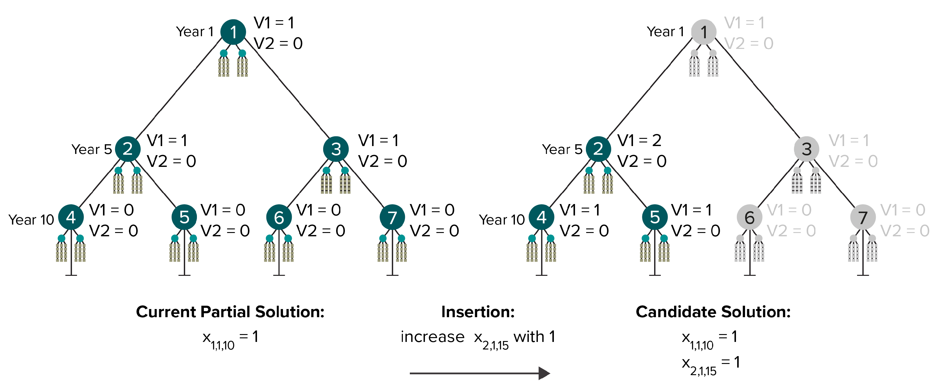
Figure 2 illustrates a current partial solution and a candidate solution for an instance that has seven nodes and two vessel types. The current partial solution and the resulting fleet size and mix for each node is shown to the left in the figure. To the right in the figure, we consider an increase of the decision variable $x_{2,1,15}$, meaning that at node 2, the number of vessels of type 1 and with a lease length expiring in year 15 is increased by one. Only nodes 2, 4, and 5 are influenced by this change, and thus only operational scenarios connected to these nodes must be re-solved to evaluate the resulting candidate solution.

Considering similarities in strategic solutions can also allow avoiding unnecessary calculations. The deployment of a fleet in operational scenarios does not depend on how the fleet was acquired. That is, the costs of an operational scenario only depend on the total number of vessels of each type available. Strategic decisions that result in the same fleet size and mix, but differ in how vessels are acquired, are therefore equivalent when considering operational costs.

Data structures based on hashing are therefore used to avoid resolving operational scenarios where the cost of deploying a given fleet has already been calculated. That is, we store the operational cost of deploying a given fleet in all scenarios belonging to a given node and season type combination. When executing the fleet deployment heuristic to evaluate a given candidate solution, the hashing-based data structure is queried to check whether the operational scenarios have already been solved with the same fleet. The execution of the fleet deployment heuristic can thereby be skipped both for the strategic nodes that are unaffected by the considered insertion and for the strategic nodes where the same fleet has already been evaluated from an operational perspective.

4. Computational Study

The tests reported in the computational study have been performed on a computer with two 2.4 GHz Intel CPUs, 10 cores, and 96 Gb RAM. The GRASP heuristic was implemented in the Java programming language. The performance of the fleet deployment heuristic used to solve operational subproblems is analyzed in Section 4.1. Section 4.2 reports on the calibration of the parameters of the reactive GRASP. The main results for evaluating the effectiveness of the proposed GRASP are shown in Section 4.3.

4.1. Performance of the Fleet Deployment Heuristic

The performance of the fleet deployment heuristic is vital for the overall performance of the GRASP, since it heavily affects the evaluation of candidate insertions when constructing solutions. In this section, the results of the fleet deployment heuristic are compared to the optimal solutions of operational scenarios given by solving a mathematical model [1] using a commercial MIP solver.

We do not expect that a simple greedy heuristic can find the exact same decisions as when solving a model with perfect look-ahead to optimality. However, we may hope that applying the heuristic to different fleet size and mix combinations will result in a similar ranking of the fleets as when applying the MIP solver.

To identify and analyze any differences between the optimal operational decisions and the results of the fleet deployment heuristic, we solve a set of test instances where the strategic decisions have been fixed. The operational decisions made by the two solution methods are then inspected and compared.

For the evaluation, we consider four test cases, each including ten different test instances. Each test case has a single strategic node and 120 operational scenarios. The test instances in the each test case differ only in the number of periods for each operational scenario. Besides comparing the operational costs, the test cases are also utilized to evaluate how the number of periods influences the differences in cost. In each test instance, the chosen fleet consists of six vessels during the summer season and four vessels during the winter season. The difference between the operational cost found by the fleet deployment heuristic and the optimal operational cost found by the MIP solver is given by:

$$\mathrm{Difference}=\frac{\mathrm{Operational}\mathrm{Cost}\left[\mathrm{Heuristic}\right]-\mathrm{Operational}\mathrm{Cost}\left[\mathrm{Solver}\right]}{\mathrm{Operational}\mathrm{Cost}\left[\mathrm{Solver}\right]}$$

(24)

A positive value represents that the fleet deployment heuristic has a higher operational cost than the MIP solver. Figure 3 reports the average differences over the 10 test instances in each test case. The average operational cost found for a given fleet is between 1.5% and 3.0% higher for the fleet deployment heuristic than for the MIP solver. The average difference is higher during the winter season than during the summer season, independently of the number of periods. Furthermore, Figure 3 also shows that the differences in operational costs are higher when the operational scenarios have only three periods.

The results imply that the fleet deployment heuristic is unable to utilize the given fleet quite as well as the MIP solver, in particular during winter. In the winter season, weather conditions are harsher and less time is available for performing maintenance operations. This makes it more beneficial to obtain an optimal fleet deployment, and the consequences of deviating from this optimal deployment are more severe. However, the decisions made by the heuristic are arguably more realistic than the decisions made by the solver, in the sense that the mathematical model used by the MIP solver has perfect knowledge about maintenance tasks that appear late in the operational planning horizon, and thus is likely to suggest decisions that could not have been realistically implemented in practice, due to actual information about maintenance tasks arriving too late for perfect plans to be formed.

As there is a slight difference in both decisions and operational costs reported by the heuristic and the MIP solver, further analysis is undertaken to check whether these differences influence what is considered to be the best fleets in the given situations. The following testing aims to evaluate whether both solution methods lead to the same conclusions regarding which fleet size and mix decisions are better or worse. We would like to see that a solution which is considered to be good (low objective value) by the MIP solver is also considered good by the fleet deployment heuristic, and vice versa.

To this end, we consider ten different fleet size and mix solutions (fleets) for a single test instance with one strategic node and 120 operational scenarios spanning ten periods each. Both solution methods are applied to find operational decisions for each fixed fleet.

Table 1. Ranking of fleets according to objective function value.

	MIP Solver		Fleet Deployment Heuristic
Fleet	Objective [m€]	Rank [-]	Objective [m€]	Rank [-]	Difference [%]
1	73.77	1	74.32	1	1.70
2	74.02	2	74.37	2	1.13
3	74.11	3	74.54	3	1.36
4	75.60	4	76.86	5	3.65
5	75.64	5	76.90	6	3.57
6	76.43	6	76.84	4	1.33
7	82.10	7	83.56	7	3.55
8	114.89	8	117.78	8	3.76
9	201.22	9	207.26	9	3.65
10	1550.64	10	1550.64	10	0.00

shows the objective function values obtained and the solution methods for each of the different fleets. The table also indicates how the different fleets are ranked by each solution method. The rightmost column provides the differences in the operational costs using Equation (24).

Table 1 shows that the MIP solver and the greedy heuristic both rank the best and the worst fleet size and mix solutions equally, with seven of the ten fleets having the same rank according to both solution methods. In particular, the three best fleets and the four worst fleets all have identical ranks. There is only one fleet that leads to any differences in ranks: the sixth best fleet according to optimal costs is ranked as number four when applying the heuristic, whereas all other fleets are ranked in the same order as with optimal costs. Since fleets 4 to 6 are all very similar in terms of their objective function values, this an acceptable result and the fleet deployment heuristic’s performance is considered sufficiently good for its intended use within the GRASP.

4.2. Calibration of the Reactive GRASP

When solving the DLPOW using the reactive GRASP, the performance of the heuristic is affected by several parameters. As presented in Section 3.1, this includes Max_Iterations, Top_Down, Rank_Based, $\delta$, $A=\{{\alpha }_1,\dots ,{\alpha }_m\}$, and $I^B$. Both the quality of the solutions and the computational time of running the GRASP are affected by these parameters. Calibration testing is used to evaluate combinations of parameter values and determine the best performing combination. Such testing has been executed by considering the parameters in a sequential manner, changing one parameter at a time while keeping the other parameters fixed at reasonable values.

Ten test instances were used to calibrate the GRASP. These instances have between one and thirteen strategic nodes which form strategic scenario trees with varying shapes. Different types of strategic uncertainty are considered in these instances, either without strategic uncertainty (Deterministic), with uncertainty in the price of electricity (Electricity Price), or with uncertainty in the step-wise development of wind farms (Farms). The instances have either four or six vessel types, and either two or three wind farms. Stålhane et al. [1] found that 120 operational scenarios with ten periods each is appropriate, and all the test instances used for calibration adhere to this setting. The test instances used for parameter calibration are summarized in

Table 2. Test instances used in the calibration testing of the GRASP. The strategic scenario trees for instances marked with an asterisk are unbalaned. Their structure is explained in [1].

Instance Name	Strategic Uncertainty	# Nodes at Each Stage	# Strategic Nodes	# Vessel Types (# Stations)	# Farms (# Turbines)
T1	Deterministic	(1, 1, 1)	3	4 (2)	2 (200)
T2	Deterministic	(1, 1, 1, 1, 1)	5	4 (2)	2 (200)
T3	Farms	(1, 2, 3) *	6	4 (2)	3 (300)
T4	Farms	(1, 3, 6) *	10	4 (2)	3 (300)
T5	Electricity Price	(1, 2)	3	4 (2)	2 (200)
T6	Electricity Price	(1, 2, 4)	7	6 (3)	2 (200)
T7	Deterministic	(1, 1, 1)	3	6 (3)	2 (200)
T8	Farms	(1, 3, 6) *	10	6 (3)	3 (300)
T9	Electricity Price	(1, 3)	4	6 (3)	2 (200)
T10	Electricity Price	(1, 3, 9)	13	6 (3)	2 (200)

.

Two variants of the reactive GRASP are considered: an any-node reactive GRASP (ANG) and a top-down reactive GRASP (TDG). These variants are different in how candidate insertions are defined and solutions are built, and the best values of the different parameters are likely to be different as well. Therefore, the parameters are tuned separately for ANG and TDG. Systematic testing was conducted for the parameters Rank_Based, $A=\{{\alpha }_1,\dots ,{\alpha }_m\}$, and Max_Iterations, while $\delta$ is set to 10 as proposed by Prais and Ribeiro [13] and $I^B=10$ based on preliminary tests. The parameter tuning took place in three phases, with different parameters being calibrated in each phase.

In the first phase, the effect of rank-based and value-based selection of the RCL influenced the performance of the GRASP. Each of the ten test instances was considered twice for both the TDG and the ANG, using rank-based selection and value-based selection one time each. For this phase, the GRASP used Max_Iterations = 1000, and $\alpha$-values were drawn from the set $A=\{0.00,0.10,0.20,\dots ,1.00\}$. The value-based selection outperforms the rank-based selection both in terms of total computational time and the time to reach the best solution found. All following tests therefore applied a value-based RCL selection.

The second phase considered the parameters related to the reactive aspect of the GRASP, aiming to determine an appropriate set of $\alpha$-values. This entailed determining an appropriate maximum value for $\alpha$, and a suitable number of equidistant values from which to select. Again using both TGD and ANG, the maximum value for $\alpha$ and the distance between the values were varied, while simultaneously keeping the minimum value of $\alpha$ at zero. In the tests conducted for the first phase, we noticed that the best solutions were always found for $\alpha$-values in the range 0.00–0.20. Based on this, both TGD and ANG were tested with a maximum $\alpha$-value of 0.20, and two alternative sets of alphas were tested: $A_1=\{0.00,0.10,0.20\}$ and $A_2=\{0.00,0.05,0.10,0.15,0.20\}$.

The results revealed that adjusting the maximum of $\alpha$ from 1.00 to 0.20 did not harm the quality of solutions found by the GRASP variants. The same solutions were identified with both $A_1$, $A_2$, and the original range, $A=\{0.00,0.10,\dots ,1.00\}$. However, the new and smaller sets, $A_1$ and $A_2$, led to a significant decrease in the computational time required to find these solutions. It was observed that the same solutions were sometimes found for different $\alpha$-values, which implies that the GRASP is relatively robust with respect to this parameter. For further testing, the set $A_2$ was selected, as it provided a slight increase in the flexibility and potential diversification of the search, while not causing any additional increase in the computational time.

The third phase of the parameter tuning focused on setting the maximum number of iterations, Max_Iterations. Given that test instances differ significantly in terms of size and complexity, the number of iterations required to identify high-quality solutions may vary from instance to instance. The number of vessel types and strategic nodes in an instance are both expected to affect the number of iterations required, as both directly influence the number of valid candidate insertions to evaluate per iteration. Instead of deciding on one specific value of the maximum iterations to use for all of the test instances, the number of iterations was set as a function of the problem size, thereby allowing the GRASP to spend a higher number of iterations when solving larger test instances. The number of iterations is then a function: Max_Iterations = strategic nodes × vessel types ×$\beta$, where $\beta$ is a parameter whose value must be determined.

The outcome of the third phase reveals that all $\beta$-values above 0.5 led to good solutions with a relatively low number of maximum iterations. Thus, for all further testing, a value of $\beta =0.75$ was selected, providing a good trade-off between solution quality and computational time.

4.3. Performance of GRASP

To evaluate the performance of the GRASP for DLPOW, it is compared to the best solutions obtained by exact methods in [1]. The exact methods, including using a MIP solver on a direct formulation of the problem, as well as an ad hoc integer L-shaped method, were each run for a maximum of 43,200 s on the same hardware as used for running the GRASP. The comparison is made on 33 different test instances. All instances have 120 operational scenarios with ten periods in each strategic node, but the size of the test instances vary greatly. The number of strategic nodes vary from 1 to 63, structured in strategic scenario trees of different shapes. Different sources of strategic uncertainty are taken into account within the test instances, while varying the number of wind farms, stations, and vessel types. The set of instances generated contains both instances that are intended to be fairly easy to solve, as well as instances that are created to test the limitations of the solution methods examined.

Table 3. Test instances used in the performance testing. The strategic scenario trees for instances marked with an asterisk are unbalanced. Their structure is explained in [1].

Instance Name	Strategic Uncertainty	# Nodes at Each Stage	# Strategic Nodes	# Vessel Types (# Stations)	# Farms (# Turbines)
D1	Deterministic	(1)	1	4 (2)	2 (200)
D3	Deterministic	(1, 1, 1)	3	4 (2)	2 (200)
D5	Deterministic	(1, 1, 1, 1, 1)	5	4 (2)	2 (200)
D10	Deterministic	(1, 1, 1, …, 1)	10	4 (2)	2 (200)
D25	Deterministic	(1, 1, 1, …, 1)	25	4 (2)	2 (200)
F6	Farms	(1, 2, 3) *	6	4 (2)	3 (300)
F10	Farms	(1, 3, 6) *	10	4 (2)	3 (300)
F35	Farms	(1, 3, 6, 10, 15) *	35	4 (2)	3 (300)
F56	Farms	(1, 5, 15, 35) *	56	4 (2)	3 (300)
F56${}^{\prime }$	Farms	(1, 3, 6, 10, 15, 21) *	56	4 (2)	3 (300)
EP3	Electricity Price	(1, 2)	3	4 (2)	2 (200)
EP4	Electricity Price	(1, 3)	4	4 (2)	2 (200)
EP7	Electricity Price	(1, 2, 4)	7	4 (2)	2 (200)
EP13	Electricity Price	(1, 3, 9)	13	4 (2)	2 (200)
EP21	Electricity Price	(1, 4, 16)	21	4 (2)	2 (200)
EP40	Electricity Price	(1, 3, 9, 27)	40	4 (2)	2 (200)
EP63	Electricity Price	(1, 2, 4, 8, 16, 32)	63	4 (2)	2 (200)
D1.2	Deterministic	(1)	1	6 (3)	2 (200)
D3.2	Deterministic	(1, 1, 1)	3	6 (3)	2 (200)
D5.2	Deterministic	(1, 1, 1, 1, 1)	5	6 (3)	2 (200)
D10.2	Deterministic	(1, 1, 1, …, 1)	10	6 (3)	2 (200)
D25.2	Deterministic	(1, 1, 1, …, 1)	25	6 (3)	2 (200)
F6.2	Farms	(1, 2, 3) *	6	6 (3)	3 (300)
F10.2	Farms	(1, 3, 6) *	10	6 (3)	3 (300)
F35.2	Farms	(1, 3, 6, 10, 15) *	35	6 (3)	3 (300)
F56.2	Farms	(1, 5, 15, 35) *	56	6 (3)	3 (300)
F56’.2	Farms	(1, 3, 6, 10, 15, 21) *	56	6 (3)	3 (300)
EP3.2	Electricity Price	(1, 2)	3	6 (3)	2 (200)
EP4.2	Electricity Price	(1, 3)	4	6 (3)	2 (200)
EP7.2	Electricity Price	(1, 2, 4)	7	6 (3)	2 (200)
EP13.2	Electricity Price	(1, 3, 9)	13	6 (3)	2 (200)
EP40.2	Electricity Price	(1, 3, 9, 27)	40	6 (3)	2 (200)
EP63.2	Electricity Price	(1, 2, 4, 8, 16, 32)	63	6 (3)	2 (200)

summarizes the test instances’ characteristics.

Both the TDG and the ANG were given a time limit of 2 h (7200 s), significantly less than the 12 h given to the exact methods, in addition to the limit on the maximum number of iterations.

Table 4. Solution values found by the GRASP.

	TDG			ANG
Test Instance	Total Time (s)	Difference to Primal (%)	Difference to Dual (%)	Total Time (s)	Difference to Primal (%)	Difference to Dual (%)	ANG vs. TDG (%)
D1	2	0.8	0.8	2	0.8	0.8	0.0
D3	6	1.3	1.4	6	1.3	1.4	0.0
D5	11	3.2	3.5	11	2.2	2.5	−0.9
D10	21	2.1	2.7	27	1.1	1.7	−1.0
D25	102	−3.6	15.9	144	−4.5	14.8	−1.0
F6	27	1.7	2.3	28	1.3	2.0	−0.3
F10	35	−10.6	2.5	42	−10.6	2.5	0.0
F35	204	−91.9	13.9	786	−92.0	12.2	−1.4
F56	305	NA	NA	6848	NA	NA	0.0
F56’	401	NA	NA	5221	NA	NA	−1.3
EP3	6	1.1	1.6	7	1.1	1.6	0.0
EP4	7	1.2	1.5	9	1.2	1.5	0.0
EP7	13	1.1	1.5	15	1.1	1.5	0.0
EP13	24	1.4	2.2	42	1.4	2.2	0.0
EP21	46	−4.7	13.3	94	−4.7	13.3	0.0
EP40	101	−90.9	11.6	851	−90.9	11.6	0.0
EP63	236	NA	NA	7200	NA	NA	−0.9
D1.2	3	0.7	0.9	4	0.7	0.9	0.0
D3.2	11	0.7	1.0	17	0.7	1.0	0.0
D5.2	26	2.1	2.5	29	1.2	1.6	−0.9
D10.2	45	1.4	2.2	68	0.9	1.7	−0.5
D25.2	326	−15.4	15.4	407	−16.9	13.3	−1.8
F6.2	46	0.0	3.1	48	−0.8	2.2	−0.8
F10.2	84	−16.7	11.0	107	−16.7	11.0	0.0
F35.2	626	−95.3	14.1	1990	−95.4	12.5	−1.4
F56.2	745	NA	NA	7200	NA	NA	0.0
F56’.2	1032	NA	NA	7200	NA	NA	−1.5
EP3.2	12	0.8	1.7	10	0.8	1.7	0.0
EP4.2	18	0.7	1.0	17	0.7	1.0	0.0
EP7.2	27	0.6	1.4	35	0.6	1.4	0.0
EP13.2	60	0.9	2.4	91	0.9	2.4	0.0
EP40.2	295	−26.4	14.5	1968	−26.4	14.5	0.0
EP63.2	866	NA	NA	7200	NA	NA	−0.9

shows the main results from running the TDG and ANG versions of GRASP on the instances listed in Table 3. For each of TDG and ANG, we report the total time used in seconds, and the difference between the best solution found by the heuristic and the best known primal and dual bounds obtained by the exact methods by Stålhane et al. [1]. The rightmost column compares the objective function values of the best solutions found by ANG and TDG, with negative values indicating that ANG has found a better solution.

Table 4 shows that the TDG and the ANG are both able to find feasible solutions to all of the instances tested, within the two-hour time limit. Hence, they enable solving much larger instances than the exact methods can handle, with a much smaller computational budget. Out of the 27 instances for which the exact methods find a feasible solution, GRASP identifies better solutions for the ten largest test instances, improving the objective function values by between 0.8% and 95.4%. However, for the 17 smallest instances, applying the GRASP leads to slightly worse solutions, with up to 2.2% increased cost compared to the exact methods.

For the test instances where the exact methods provide a lower bound, making it possible to calculate an optimality gap, the solutions found by the GRASP are within 15.9% of optimality. This is a large gap, but the dual bounds found by the exact methods are likely to be poor for the larger instances. Hence, a large difference to the lower bound for the GRASP solution does not imply that the solution found is necessarily much worse than an optimal solution.

The ANG finds better solutions than the TDG for 14 of 33 instance, whereas the TDG does not find better solutions than the ANG for any instance. However, the differences in the objective function values found by the two solution methods are relatively small, ranging from 0.0 to 1.8%. The difference in computational time is insignificant for instances with few strategic nodes. However, TDG is much faster than the ANG for some of the larger instances.

To conclude, the GRASP outperforms the exact methods both in terms of solution quality and solution time when solving the DLPOW. That is, for all but the smallest instances, which are the least realistic instances in terms of size, the solutions found by the GRASP are better than those of the exact solution methods. The two GRASP variants have similar performances, but while ANG finds slightly better solutions than TDG for some instances, the computational effort required by the ANG is larger than for TDG when considering large instances. Both GRASP versions are thus considered as providing a promising performance.

5. Concluding Remarks

This work studied a strategic fleet size and mix problem for conducting maintenance at offshore wind farms. The dual-level fleet size and mix problem for conducting maintenance at offshore wind farms (DLPOW) was defined by Stålhane et al. [1], and accounts for both short-term operational uncertainty and long-term strategic uncertainty by combining decisions with two different timescales in a dual-level stochastic optimization model. Solving the DLPOW can support wind farm owners when making strategic decisions regarding vessels to charter in the long-term and short-term, in order to meet the demands for maintenance throughout a wind farm’s lifetime. The DLPOW also takes into account the cost of deploying the fleet to perform maintenance activities in light of uncertain demand for maintenance and uncertain weather conditions.

Previous work used a standard MIP solver directly on a mathematical formulation of the DLPOW, as well as an ad hoc integer L-shaped method [1]. Extensive tests showed that the exact methods are impractical to use except when solving small problem instances.

Therefore, we developed a heuristic solution method based on GRASP to provide approximate solutions of the DLPOW. Our reactive GRASP heuristic is designed to exploit the block-separable structure of the problem at hand, which then decomposes into a master problem and a set of independent subproblems. The heuristic constructs strategic fleet size and mix solutions to solve the master problem, and a simple embedded fleet deployment heuristic is used to solve the subproblems of operational fleet deployment, thereby providing an objective function value for a given fleet size and mix solution. Two versions of the reactive GRASP were developed, with a top-down version being more restricted in terms of constructing solutions than an any-node version.

Extensive testing was conducted. Independent testing of the embedded fleet deployment heuristic showed that the heuristic performs well for its use, being able to rank different fleet size and mix solutions in approximately the same order as when using an MIP solver and finding deployment decisions that are close to optimal in terms of cost.

Parameter tuning for the reactive GRASP showed that the method is robust with respect to parameter values. The performance of the GRASP was compared to the best solutions obtained by two exact methods that were given a higher computational budget. Test results indicated that the GRASP consistently produces high-quality solutions for the DLPOW. The GRASP, compared to the exact methods, identifies much better fleet size and mix solutions for all but the smallest test instances.

While the proposed solution method is based exclusively on GRASP, with no local search component, there could be ways to exploit local search to improve the overall search when solving problems based on a scenario tree structure. The important decisions are the here-and-now decisions, while the other decisions at other nodes than the root node are mainly important for evaluating the quality of the here-and-now decisions. Therefore, we propose a local search that examines small changes in the decisions in the root node only. Since these changes are disruptive, to evaluate a neighboring solution, GRASP could be used to construct the solution below the root node in the scenario tree. This could be more effective than simply using GRASP from scratch each time. However, we leave this as future research.