
Port Terminal Performance Evaluation and Modeling


1
School of Transportation and Logistics Engineering, Wuhan University of Technology, Wuhan 430063, China
2
National Engineering Research Center for Water Transport Safety, Intelligent Transport System (ITS), Wuhan 430063, China
*
Author to whom correspondence should be addressed.
Logistics 2022, 6(1), 10; https://doi.org/10.3390/logistics6010010
Submission received: 21 December 2021
/
Revised: 11 January 2022
/
Accepted: 14 January 2022
/
Published: 20 January 2022
/
Retracted: 3 March 2023
Abstract
:Background: The efficiency and competitiveness of port supply chain entities are two critical concerns for maritime transport that must constantly be enhanced. This paper presents an approach called ECOGRAISIM for evaluating the performance of the seaport supply chain. The objective is to achieve an effective operational plan for multimodal terminals. Methods: The proposed approach incorporates the ECOGRAI (Graph with Interconnected Results and Activities) technique with ESSIMAS (Evaluation by Simulation of Innovative Solutions for the Development of Mass Transport on the Seine Axis by electric rail coupons). An additional stage was incorporated to accomplish the performance control. A particular focus was put on action variables and procedures for container and massified transfer management. The multimodal terminal at Le Havre seaport was adopted as the case study. Results: Several scenarios of container transfer were defined and investigated based upon specific features, including delays, minimizing expenses and CO2 emissions. The results show that the operational planning method results in a higher service rate and significantly reduces delay, cost and CO2 emissions. Conclusions: The proposed approach is bound to be beneficial for maritime transport planners and decision makers.
1. Introduction
A port’s logistics chain performance is determined by decisions made at the strategic, tactical and operational level [1]. Our research focuses on evaluating the efficacy of various methods of rail container transfer between the terminals of the Port of Le Havre in order to improve container fluidity while lowering costs and CO2 emissions.
Specifically, we are interested in the performance of container transit massification via the multimodal terminal in Le Havre. The goal of the multimodal terminal is to raise the modal share of mass transportation in France, which lags substantially behind competitive ports in northern Europe. Multimodality allows for increased competitiveness as well as greater respect for the environmental [1,2]. From an environmental standpoint, the goal is to reduce road traffic by increasing usage of rail and river transportation. Rail shuttles transport containers between the maritime terminals and the multimodal terminal in Le Havre, which is an important aspect of the port’s competitiveness. Furthermore, in order to improve the fluidity of container traffic it is vital to understand how to adjust the flow of existing means.
Our goal is to achieve an efficient multimodal terminal operating process in terms of several performance indicators: resource occupancy rate, container delivery on-time service rate and inefficient movement number. It is possible to monitor performance indicators and evaluate performance by simulating various transfer mechanisms.
2. Literature Review
Much of the research focuses on performance evaluations. The National Center for Textual and Lexical Resources defines “performance” as the measure of a participant’s ultimate outcome [2]. It considers a number of aspects, such as cost, improvement, service quality, punctuality and work-life balance. The profitability of a container terminal at a port is inextricably related to the port’s investment costs and productivity [3].
The ability of container terminals to maintain an uninterrupted flow of information and activities is highly valued in the supply chain. A performance indicator is a piece of data that assists a decision maker or group in making the appropriate decisions to attain the established goals. The set of performance indicators for the logistics industry aims to assess the efficiency and viability of the system and covers all levels of decision making: strategic, tactical and operational [4].
Port performance indicators are used to track how management rules are being followed and to identify areas for improvement [5]. Performance indicators are never final, as fluid user demands and objectives continually necessitate their reevaluation [4]. Performance indicators must be SMART (specific, measurable, realistic, reasonable and time-bound), also known as intelligent performance indicators [5]. There are two categories of performance indicators: those that indicate whether or not a goal has been met and those that offer information on a specific process. For example, an indicator that tells us the handling rate of containers per hour in a terminal will lower if a decline happens, prompting us to investigate the source and make the required decisions [6].
Gaugris divides performance measures into three categories: growth rate, ratios and contribution indicators [5]. Depending on the sort of organization analyzed, we may identify two categories of people: financial and non-financial. The authors of [4] outline both quantitative and qualitative indicators. Such indicators cover various activities such as storage and transportation and financial indicators such as rate of return, revenue, profit and sale price [7,8].
Flow simulation is a frequently used method for creating a model that represents a real-world system. Simulation has historically been used to create or modify manufacturing units, and it is still used to manage production systems. As the logistics chain evolves, new applications for flow modeling emerge [9]. Simulation allows for the evaluation of a real system’s performance and behavior attributes through a virtual representation. For example, it may be used to estimate the size of the system, increase equipment use and illustrate the potential of additional equipment. Dynamic modeling of business behavior under various degrees of constraints and diverse policies is possible using simulation-based methodologies [10].
3. Scope of the Study and Issues
The multimodal terminal is intended to accommodate containers through rail shuttles from various freight forwarding sites, such as marine terminals and industrial and logistical areas. It contains areas and handling equipment for transferring containers to barges and mainline trains, as well as possible interim storage.
The scope of the study includes the Atlantic Terminal, the Terminal de France (TDF), the Terminal de la Porte Océane (TPO) and the Mediterranean Shipping Company’s Normandy Terminals. A rail link connects these terminals to the multimodal terminal.
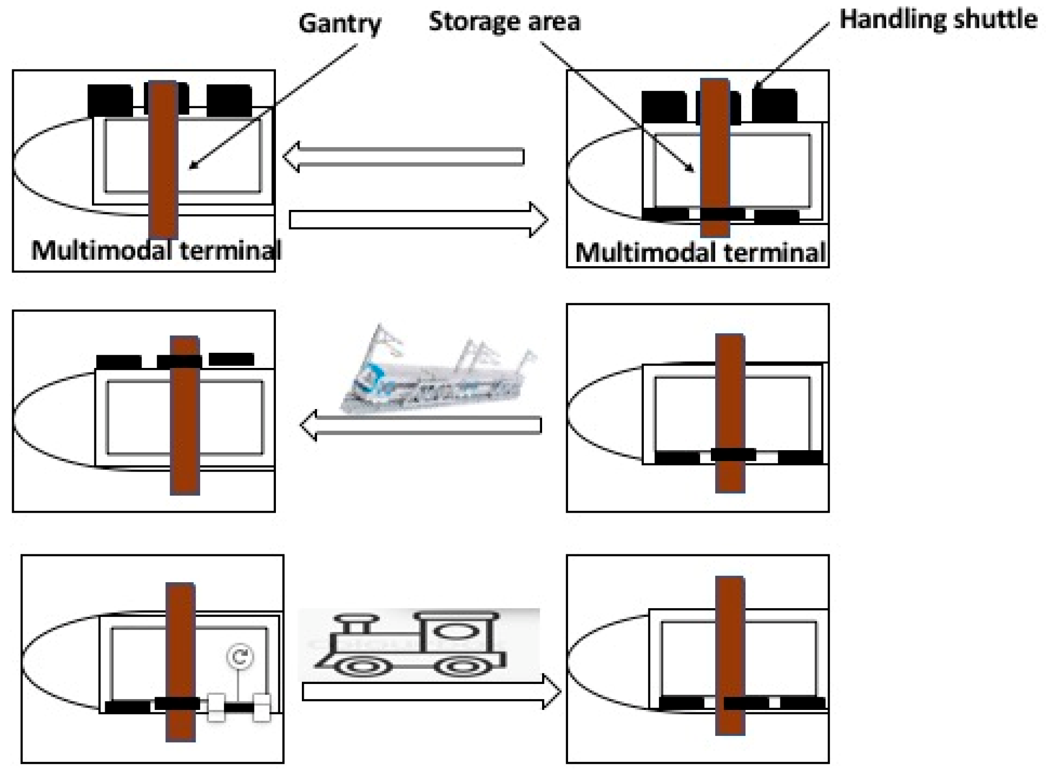
The containers are accepted at a marine terminal and subsequently collected from the storage area during import. To ensure the transfer to the multimodal terminal, a shuttle must be positioned, containers must be loaded, a locomotive must be hitched and the shuttle must be started [11]. When the shuttle arrives at the multimodal terminal, it will be directed based on its destination: rail platform, river platform or both platforms, as well as track availability (otherwise it must wait at the reception beam). If there isn’t a crane available, the shuttle must wait on the track.
Export containers will be received at the multimodal terminal and transferred to a maritime terminal compatible with the import of containers. The stages of a transfer operation from a maritime port to a multimodal terminal are depicted in Figure 1.
A Unified Modeling Language (UML) was used to model the container handling and transfer processes by rail shuttles [12]. The modeling focuses on the processes of shuttle composition that ensure container transfer between terminals, the processes of railway maneuvers for shuttle movement and the processes of transport unit loading and unloading (barges, mainline trains and shuttles railways).
4. Development of a Simulation System
Several simulation tools are available commercially for developing a simulation system (Table 1).
We used FlexSim CT (Container Terminal) software to execute our discrete event simulation model. FlexSim CT is designed to represent and simulate the evolution of real traffic in ports.
4.1. Demonstration of FlexSim
FlexSim Software Products was formed in 1993 by Bill Nordgren, Roger Hullinger and Cliff King as F&H Simulations. In the year 2000, the company’s name was changed to FlexSim.
FlexSim provides numerous tools for modifying development, and allows presentation in 3D mode. It is an object-oriented tool that uses its CT (Container Terminal) library to model and simulate container flows in port terminals and port transit processes. C++ or FlexScript is used for programming. Each object in FlexSim has its own graphical user interface (GUI) that is used to model it.
FlexSim CT, however, deals solely with operations within the maritime port and therefore does not permit the building of railways. To overcome this, we utilized a library designed specifically for rail transportation.
4.2. Presentation of the Rail API Library
Anthony Johnson created the Rail API in 2008 to allow for the implementation of articulated movements of railcars. The library is a set of commands that allows users to create trains and move them along the tracks of a rail network. The API is used to handle train traffic and shuttle activity. The following are the primary API functions that we used:
Create rail sequence: used to build and return a reference to a rail sequence. A rail sequence is a collection of activities that include moving, sending a message, delaying and waiting. These operations are carried out on a set of objects (travelers). Thus, a rail sequence facilitates the transportation of a collection of wagons on a rail network from point A to point B.
Create rail path: a path for creating railways.
Add rail move: to move a shuttle from one network node to another, parameters such as speed, acceleration, deceleration, start point and stop point must be specified.
Add rail message: this function is used to communicate messages between objects. When a shuttle arrives at a handling site, for example, the handling machine object receives a message to begin handling and sends a return message to release the other resources involved then proceed to the next task.
The Rail API’s different functions allow users to add actions to a sequence established by the create rail sequence function, for example, moves, waiting times, pauses and message sending by using the functions “add rail move”, “add rail delay”, “add rail wait” and “add rail send message”, respectively.
4.3. Implementation
In the FlexSim software, we locate the objects described in the UML modeling on which we relied to simulate the resources of our model (Figure 2):
- Storage spaces (Yard): While FlexSim CT does not allow the inclusion of the yard object without previously preparing the arrival or departure of a boat or truck, we have modeled a storage area with a horizontal rack.
- Container storage cranes (Gantry Crane): Because the “Gantry Crane” object only works in a yard, we used the crane object, which serves as a gantry crane.
- Container: Made with the “Basic TE” object.
- Wagons and rails: Using the API Rail library
FlexSim also has the presence of “triggers” on some objects; triggers react to numerous events that occur on the object in question. Our model, too, has distinct triggers. These triggers contain FlexScript code.
We have completed the implementation of the business objects mentioned previously. Their mission is to manage numerous activities, including such things as handling, track management and shuttle movement. The usage of the coordination objects approach was also driven by the fact that FlexSim is primarily centered on sending messages; this allows for communication between the different objects, making it easier to coordinate the various actions (Figure 2).
The simulation model created (Figure 3 includes the multimodal terminal as well as the set of maritime terminals in question. The multimodal terminal is made up of a reception beam, a railway yard for mainline trains, a river yard for barges and connecting tracks for locotractors.
4.3.1. Beam Reception
The beam reception is entirely electric. As a result, mainline trains can travel directly there. The locomotive is uncoupled in order to proceed to a siding. A locomotive attaches to the wagons and transports them to the rail yard. When the train is reloaded, the line locomotive arrives directly to the rail yard—the beam head of which is electrified—attaches itself to the wagons, and the train can go without passing through the receiving beam. If the shuttles are unable to proceed directly to the railway yard or river yard, they will come to a halt on the receiving beam. The trains (a train is a collection of coupons without a locomotive) are then redistributed on the tracks and in the river yard by the locomotive. The principle is the same in the opposite direction.
4.3.2. Train Station
The railway yard is made up of eight parallel lines. It has two railway gantries for transferring cargo from trains to shuttles and vice versa. The distribution of trains and shuttles on the railway yard is customizable. To better handle line trains arriving at a multimodal terminal, a priority is allocated to each train, taking into account the delivery times set for the containers they convey.
4.3.3. River Court
Under the gantry, four lanes are utilized for unloading and loading import-export containers from shuttles.
4.3.4. Container-Shipping Facilities
Atlantic Terminal, Terminal de France (TDF), “Terminal de la Porte Océane” (TPO) and Terminal de Normandie of the Mediterranean Shipping Company are the maritime terminals that have been implemented (TNMSC). The simulation is limited to maritime terminal buffers within the framework of the two ESSIMAS and DCAS programs. See (Figure 2 and Figure 3).
5. Simulation Scenarios
The performance indicators are determined using the ECOGRAISIM technique, with the goal of linking the action variables to both these indicators and the objectives [10]. It is thus necessary to evaluate the determined performance indicators and test various mechanisms of internal container transfer. Then, using simulation, we conducted a study to compare two operating modes: planned mode and massed mode. To begin with, the simulation’s major goal is to manage container movement between the multipurpose terminal and the ocean marine port while meeting delivery deadlines and minimizing resource expenditures [13,14]. Operational indicators here allow decision makers to plan and assess long-term outcomes. A single performance metric cannot suffice due to the terminal’s complexity and the high number of participants involved in its functioning. The number of vessel arrivals and time spent at the dock, as well as the number of containers handled each hour when the ship is docked, are the most commonly utilized indicators.
5.1. Massified/Planned Transfer Modes
In this simulation, containers will be transferred by train from a multipurpose port to a maritime port on the Atlantic Ocean. The objective is to compare two transfer scenarios in import and export. The objective is not to optimize the sizing of resources, as the number of resources is fixed, but rather to study their interaction.
- Scenario 1: Known as “planned mode,” it entails adhering to the delivery dates of the containers; in reality, our system begins handling containers with the same departure time.
- Scenario 2: The mass mode concept is used here, if the fixed filling rate is not met, the shuttle will not leave.
When time and resources are taken into consideration, a comparison of the two exploitation modalities can be made to see which one minimizes delays, expenses and emissions. It is also important to decrease the time between when something is expected to be delivered and when it actually arrives [15]. The research was conducted according to the following guidelines:
- There is only one feasible destination at the multimodal terminal (despite the fact that there is a receiving beam, a railway yard and a river yard).
- On each terminal, there’s only room for a single buffer.
- To put it another way, the movement of containers can be compared to a series of “production” procedures that need time and resources to complete.
After the various objects were included and configured for the Port of Le Havre, two railway lines between the multipurpose terminal and the ocean marine warehouse were created, and an Excel file with the data was fed into the model (container numbers, types of containers and hours of availability) [16].
Three locomotives were employed. For a train of 25 cars, the travel time between terminals was 60 min, the maneuvering time was 30, the handling time was 3 and the filling rate for a shuttle’s departure was regulated at 80 percent.
Both the planned and the massed scenarios simulated a normal day in detail. The performance metrics to look at included the utilization rate of resources, the recurrence of inefficient movements, the number of late containers transferred and the number of delivered containers.
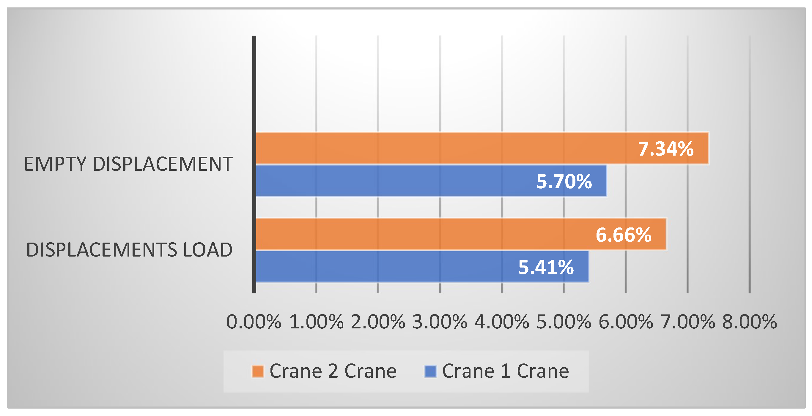
Table 2 shows the percentage of use and the percentage of unoccupied or blocked quay cranes. Thus, we can measure the performance indicators “rate of unproductive trips” and “occupancy rate”.
The “handling equipment occupancy rate” performance indicator shown in the table shows that cranes were in use around 11% to 14% of the time. “Crane1” of the multipurpose terminal was at 11.12%, including 5.70% of empty displacement (not handling a container) and 5.42% of loaded displacement. “Crane2” was operated 14% of the time at the ocean maritime terminal, with 7% of that time being empty and the remaining 6.66% filled.
During the simulation, we observed that a locomotive made a journey without cars from the multimodal terminal to the Atlantic terminal. There is a significant negative to the planned mode because resource occupancy is not optimized (Figure 4).
The massified mode’s guiding notion is to maintain a constant filling rate for the shuttles. The shuttle does not depart until it has reached 80 percent of its maximum capacity [16]. This maximizes the rate of resource usage and, in particular, the rate of utilization of the most expensive locomotives. The occupancy rate of the cranes appears to be decreasing. In reality, the occupancy rate ranged between 9 and 11 percent. The multimodal terminal’s “Crane1” is used 9.46 percent of the time, with 4.79 percent empty displacement (without containers) and 4.67 percent loaded displacement. “Crane2” at the Atlantic maritime terminal is operational 10.94 percent of the time; it is empty 5.58 percent of the time and loaded 5.36 percent of the time (Table 3). (Figure 5).
At the end of the simulation, the same number of containers (165) were transferred in order to facilitate transport from the multimodal terminal to the Atlantic terminal and vice versa. The last shuttle arrived on time in planned mode [17,18]. This aids in ensuring that all containers are moved on time. This way of operation has an advantage in terms of the performance metric “number of containers transferred late.” It ensures that no containers arrive late at the conclusion of the day. In mass mode, there were containers delivered at the end of the day (final shuttle) when they were supposed to be delivered at 3 p.m. The filling rate is to blame for the delay.
By comparing the two operating modes, we discovered that the handling occupancy rate of equipment was higher in the planned mode, while the locomotives occupancy rate was higher in the massed style. It should be highlighted that the proportion of time which resources are occupied has a direct impact on reducing costs and optimizing working time [19]. Reducing the percentage of CO2 emissions necessitates reducing the number of trips and inefficient movements and increasing the occupancy rate. In terms of service rate (number of containers delivered on time/number of containers delivered), the scheduled mode outperformed the bulk method [20]. Failure to leave before the tank reached 80 percent capacity, on the other hand, resulted in a significant delay at the end of the day [21,22].
The simulation of the two modes, mass and planned, revealed that the planned mode has a higher service rate. The planned mode is also more effective at lowering CO2 emissions. The massified mode is more cost-effective since it allows containers to be transported with fewer resources (expensive locomotives).
5.2. Optimized Transfer Mode
Simulation’s strength is its capacity to depict a system while incorporating the stochastic feature. However, it is difficult to determine the appropriate values of the decision criteria [14]. We suggest a system comprised of two modules (Figure 6): an optimization module and a simulation module [17].
Our goal was to identify the most cost-effective technique for transporting a set of containers between two container terminals [23]. To address this, we implemented an efficient exploitation technique [24]. We prepared shuttles handled at each terminal so that they could be handled without mobilizing the locomotives (Figure 7).
The simulation was fed data from an Excel sheet, which provided the following information for each container: time of availability, identifier, container type, terminals for departure and arrival.
The initial purpose of our simulation model was to test various scenarios (mass mode and planned mode) of export/import. The choice factors and number of locomotives, vehicles number and trips were roughly estimated. To compensate for this shortcoming, we chose optimization to ideally adjust these variables.
We offer our mathematical formulation below to maximize the number of import/export containers, shuttle wagons and locomotive trips.
Data:
: Locomotive cost per hour
Wagon renting cost
R: All shuttles
N R: Maximum shuttle returns number
NA: Maximum shuttle trips number
TR: Maximum shuttle size
T: Minimum shuttle size
NCX: export containers number
NCI: import containers number
Variables decision:
: Dimension of shuttle i
: Number of trips of shuttle i, from multimodal terminal to Atlantic terminal
: Number of returns of shuttle i, from Atlantic terminal to multipurpose terminal
The objective function:
We aimed to reduce the cost of using the wagons (first phrase) as well as the cost of locomotive excursions (second phrase).
Constraints:
These constraints guarantee that the volume of traffic performed by the sized shuttles is adequate for container movement (import and export)
Constraint (3) limits the size of the shuttles. In reality, the size of the shuttles is limited due to railway system constraints, notably the restricted length of the reception panels at each terminal’s entry and the limitations associated with the use of certain handling equipment (horse-drawn carriages in particular).
The number of journeys for each shuttle is limited by constraints (4) and (5). Due to human resource constraints, a locomotive can only perform a certain number of journeys every day (two shifts per day).
These constraints express the shuttles’ rotation; in actuality, the shuttles alternate between outgoing and return journeys, as well as handling at the marine port and the multipurpose terminal. Because the shuttles transfer in a “Noria” pattern, a train either has the same displacement as the others or more or less one displacement than the others.
Constraint (9) is a variable integrity constraint:
The model described is a quadratic mathematical program with integer constraints. No typical solver can solve this mathematical problem if the matrix associated with the quadratic form of constraints (1) and (2) is not positive semi-definite.
As a result, we converted the initial mathematical program into a variable program (0, 1) by writing each integer variable as a sum of powers of 2.
Given ’s integer variables:
as
with .
We construct a 0-1 program with quadratic constraints by changing the integer decision variables in constraints (1) and (2). Finally, given the following property, we obtain an alternating linear and non-linear program that we can solve with CPLEX:
Numerical Results of Optimized Mode
The CPLEX solver was successful in resolving all instances of the issue. Table 4 shows the objective function values of each instance:
Columns 1 and 2 show the numbers of containers exported and imported, respectively.
The value of the goal function for the current operation is shown in Column 3, and Column 4 shows the actual responses, which were calculated using the estimated costs of running the locomotive and renting wagons. It is estimated that over a 20-year horizon, the traffic (measured in containers) at the Atlantic Ocean terminal will account for around 10% of the total rail traffic in the Port de Le Havre. Depreciation of infrastructure and human resource costs are not included in the optimization costs [25,26].
The implemented approach is fast, with the understanding that an increase in traffic volume does not necessarily result in an increase in resolution time, as the latter is tied to the structural and temporal complexity of the problem for the instance under consideration.
The optimal mode simulation considers a normal day as well as the utilization of a single locomotive. The travel time between the two terminals is 60 min, while the handling time for each container is 3 min. For example, Figure 7 corresponds to 6 locomotive trips (a trip is a go or a return) and a total of 20 wagons for the transfer of 90 containers (the sum of the export and import containers of Instance 1).
Figure 7 depicts the evolution of the terminals’ storage spaces (the number of containers varies between 24 and 50) (Content A in blue: storage zone of the Atlantic terminal and Content M in red: storage zone of the multipurpose terminal). Figure 8 shows that the shuttles’ rotation method, “Noria”, has been followed. Each new variation (increase or decrease) in number of containers (Content A and Content M) is caused by a container loading or unloading. Furthermore, we note that the values of Content A and Content M have been reversed at the end of the simulation, indicating that all containers have been transferred on time. Furthermore, the final values of Content A and Content M allow a standard for measuring performance “service rate” to be calculated; container on-time performance is measured by the service rate (i.e., the ratio of timely containers to total containers transferred).
When we look at the numbers from the three different simulated scenarios (Figure 8, Figure 9 and Figure 10), we see that there is less variance in the terminal storage regions (in Figure 8 and Figure 9 the number of containers is between 23 and 73). The usage of the massified mode explains this variation (Figure 9). However, this method causes delays in container delivery timeframes, whereas the other two modes do not.
The comparison of the three transfer modes (planned, massed and optimized) (Table 5) reveals that the optimized and planned modes provide a greater service rate because no container is moved late. The lowering of CO2 emissions is one of the benefits of the massified mode. In small circumstances, massified mode is detrimental. The optimized mode, on the other hand, is more cost-effective because it allows the containers to be transferred with limited resources, which reduces the use highly expensive equipment [27].
It is discovered that each method of container transfer between terminals has advantages and disadvantages, but the optimum mode, which follows the “Noria” traffic pattern, allows expenses to be significantly lowered, particularly in terms of the number of locomotives. For large operations, the massified mode is strongly recommended [28].
6. Optimized Mode: Taking into Account All Terminals
This simulation provides a graphical interface (Figure 11), which is divided into tabs that allows the user to control the simulation and its parameters. The presentation tab includes a brief summary of the simulation’s aims, as well as the various interface functionalities. The next tab is divided into three sub-tabs: container management, planning, and resource sizing and placement. Container management permits users to change the number of containers that must be moved from one terminal to another. Users can define the scenario to be simulated by modifying the timetable under the planning tab. The resource sizing and placement tab configures the size of the shuttles and their starting places [29,30].
To feed our simulation, we employed a statistical approach created as part of the DCAS project. This technique adheres to the idea of circulation in “Noria” and supplies the numerous inputs required for the operation of our simulation model (Figure 11):
- -
- Three trainsets for TDF; three trainsets for TPO/TNMSC; two trainsets for Atlantic.
- -
- Scenario 1: Optimized transfer mode (5-2-5): TDF has five inputs, Atlantic has two inputs and TPO/PNMSC has five inputs.
- -
- Scenario 2: Optimized transfer mode (4-2-4): four TDF inputs, two Atlantic inputs and four TPO/PNMSC inputs.
We also provided the following management guidelines:
- Trains typically transport between 20 and 60 containers, whereas barges transport between 100 and 200 containers.
- There were two locomotives and two to six coupons for each train set: in actuality, the quantity of resources employed was defined by the most restrictive day.
Figure A1 and Figure A2 (see Appendix A) show that all of the containers were transferred by the conclusion of the day and that there were no containers in the temporary storage areas (buffers) at the end of the simulated day.
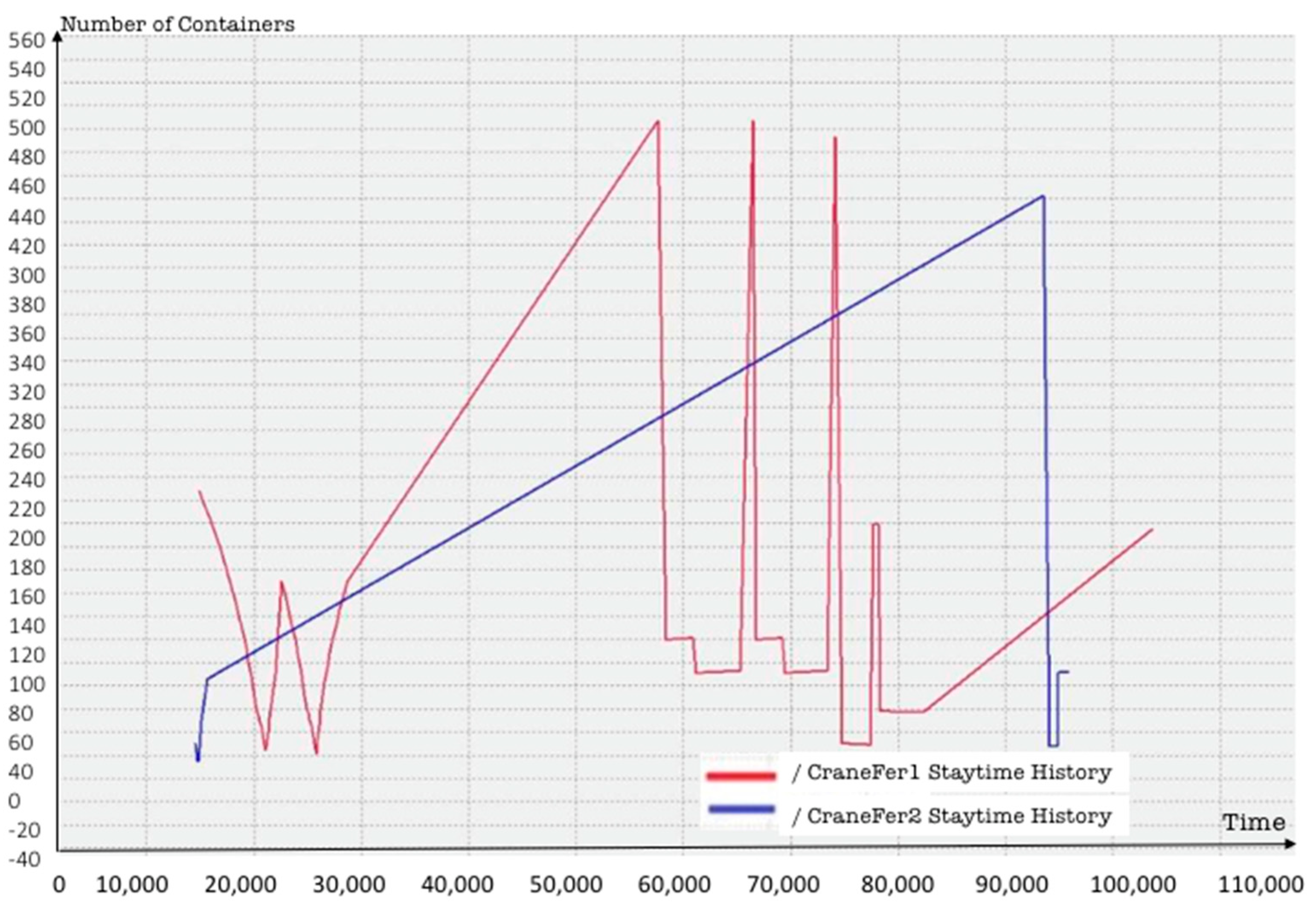
Figure A3 and Figure A4 depict the utilization rate of the multimodal terminal’s two railway gantries. We discovered a workload imbalance in both instances, with the “Crane 1” railway gantry having a higher workload than the “Crane 2” railway gantry. To better optimize (un)loading activities at the railway yard level, it would be necessary to investigate the load balancing problem.
- Offset travel empty: expresses the rate at which the railway gantry moves in the absence of a container.
- Offset travel loaded: used to express the rate of movement of the rail gantry when loaded with containers.
These two figures pertain to the multimodal terminal’s railway gantry cranes and illustrate that they were utilized optimally in Scenario 5-2-5 versus Scenario 4-2-5. This demonstrates that in the second situation there were fewer wasted motions.
In order to raise the indicator’s value, we employed an action variable “Maximize shuttle filling by serving surrounding terminals”. To examine the influence of our performance evaluation contribution on the simulation model, we measured “Resource occupancy rate”.
We discovered that using the action variable as described enhanced the simulation model when compared to rapid container evacuation. However, the model did not adhere to the restriction prohibiting the entry and exit of containers not meant for a terminal [31,32]. Additionally, the sequence diagram linked with this use case allowed for the avoidance of this error, as well as the verification of other constraints critical to correct functioning and compliance with reality. Furthermore, the sequence diagram aided in dividing functions in the model to avoid conflicts between action variables.
7. Model Validation
According to Bielli [14], the major goal of the validation process is to guarantee that the real system’s assumptions and models are logical and correctly implemented. We discovered that all containers were transferred as expected based on the numerical findings and by comparing the inputs of our simulation model with the number of containers as outputs. Then, to compare the container handling time to the actual average (3 min per container), we ran 30 simulations of the two modes and performed a Student’s t-test on the results. The goal was to determine if our population’s mean was considerably different from the true mean with a p-value of <0.05. Our population’s average time per container was 3.31 min. We examined the following scenarios:
- (1)
- Assuming H0 = 3.5 min per container and a one-sided test:
We know that our sample’s mean is less than the H0 hypothesis, so we chose the following alternative hypothesis: Mean 1: “Theoretical significance” the t-test results reveal that we cannot reject the null hypothesis H0 with a risk of error of 5%.
When the null hypothesis H0 is correct, the risk of rejecting it is 14.51%.
- (2)
- Assuming H0 = 3 min per container and a one-sided test:
Because the mean of our sample is bigger than the H0 hypothesis in this situation, we have chosen the following alternative hypothesis: The first meaning is theoretical. The findings of this t-test indicate that we must reject the null hypothesis H0 with a risk of error of 5%.
When the null hypothesis H0 is correct, the risk of rejecting it is less than 3.53%.
The different student assessments performed on our model confirmed the correctness and consistency of the simulation findings. The findings of the tests are closer to the true values.
8. Conclusions
This effort contributed to analyzing the port chain’s performance. Three container transfer techniques were studied to reduce delays, costs and CO2 emissions. The Atlantic terminal was explored as a first stage. Transport of containers was from a multimodal terminal to Le Havre’s maritime ports. Our simulation’s main goal was to control container traffic between the multipurpose terminal and the Atlantic maritime terminal while reducing resource consumption. Two management methods were considered: bulk transfer mode and scheduled transfer mode. Because there are no late containers, the scheduled mode has a greater service rate. It also outperforms the CO2 created by handling equipment. However, massing containers saves money by reducing the need for expensive resources (such as locomotives and wagons).
Following these results, we attempted to further optimize transfer by simulating a third mode. This strategy’s core idea was to utilize optimization to find the simulation’s decision variables and then simulate their performance. Several transfer mechanisms were examined (within the restraint of maintaining the “Noria” traffic pattern). Eventually all maritime ports in Le Havre adopted this method to account for multimodality at the land interface. This includes managing freight train (main line) and barge deliveries and receipts.
We sought to model, simulate and analyze the performance of port chain activities, especially at the multimodal terminal at the Port de Le Havre, to achieve efficient modes of container transfer based on our stated performance indicators. The simulation of multiple transfer modalities was used to measure performance parameters such as resource occupancy rate, service rate, number of containers delivered on time and unproductive transfers. We created ECOGRAISIM to help determine performance measures. It uses ECOGRAI and simulation to identify and assess performance indicators. The first four phases of the ECOGRAI method are utilized in ECOGRAISIM to define the performance indicators. First, we created a GRAI grid; second, we defined the decision centers’ objectives; third, we defined the decision factors. The fourth step identified the performance indicators. Following the identification of indicators, the system was modeled to duplicate its behavior. This paper also integrated optimization and simulation to identify the simulation’s decision factors.
In terms of implementation, we needed to create rail shuttle routes for export and import containers. That is, calculating resource quantities (like locomotives) and planning operations. It was represented using UML, which distinguished between functional and structural objects and coordinating and management items. Simulated container transfer modes: mass, planned and optimized modes were compared. Following the “Noria” traffic pattern was the most optimal transfer mode. To accommodate multimodality at the land interface level, all maritime ports in Le Havre adopted this method.
9. Further Studies
Other questions merit more in-depth examination, prompting us to recommend certain study avenues:
- (1)
- In order to continue working on the container transfer problem, we propose extending our simulation with further heuristics and metaheuristics to do other optimizations and simulation couplings. It would be interesting to optimize the movement of various handling equipment within the multimodal terminal in order to eliminate inefficient movements and waiting times. It is also possible to establish new modes of container transfer based on a hybridization of mass and scheduled modes.
- (2)
- Another critical area of research would simulate the many container transfer mechanisms proposed, while accounting for the uncertainty and numerous risks that may arise. It would be interesting to use the simulation model to investigate additional issues, such as the difficulty of berth allocation at the multimodal terminal’s river yard.
- (3)
- To improve the overall performance of the new logistics plan for the Port de Le Havre, we propose expanding the performance research to all GRAI decision-making centers in order to establish a complete dashboard allowing performance management from the multimodal terminal. This solution would enable the creation of performance indicator systems for all supply chain functions.
Author Contributions
G.V.M.N. and H.W., contributed to the manuscript by providing the initial concept development. G.V.M.N., was involved in the data collection and analysis. Both authors participated in writing and editing the paper. All authors have read and agreed to the published version of the manuscript.
Funding
This paper has been funded by the National Key R&D Program of China (2020YFB1712400 and 2019YFB1600400) and the National Natural Science Foundation of China (71672137).
Institutional Review Board Statement
Not applicable.
Informed Consent Statement
Not applicable.
Data Availability Statement
Data sharing not applicable.
Conflicts of Interest
The authors declare no conflict of interest.
Appendix A
The simulation of these two scenarios gave the following results:
Figure A1.
Finished container count for Scenario 4-2-4 in terms of number of containers.

Figure A2.
Number of containers at the end of the day for Scenario 5-2-5.

Figure A3.
Rate of use of the two railway gantries of the multimodal terminal for Scenario 4-2-4.

Figure A4.
Utilization rate of the two railway gantries of the multimodal terminal for Scenario 5-2-5.
Figure A4.
Utilization rate of the two railway gantries of the multimodal terminal for Scenario 5-2-5.

Figure A5.
Movement rate of the two railway gantries of the multimodal terminal for Scenario 4-2-4.

Figure A6.
Movement rate of the two railway gantries of the multimodal terminal for Scenario 5-2-5.

References
- Steenken, D.; Voss, S.; Stahlbock, R. Container terminal operation and operations research a classification and literature review. OR Spectr. 2004, 26, 3–49. [Google Scholar]
- Belin-Munier, C. Logistics, supply chain and SCM in French management journals: What strategic dimension? In Proceedings of the 23rd conference of the International Association of Strategic Management (AIMS), Rennes, France, 13 May 2014. [Google Scholar]
- Humez, V. Proposal for a Decision Support tool for Order Management in the Event of a Shortage: A Performance-Based Approach. Ph.D. Thesis, University of Toulouse, Toulouse, France, 2008. [Google Scholar]
- Lorino, P. Strategic Management Control: Management by Activities; Editions Dunod: Valenciennes, France, 1996. [Google Scholar]
- Berrah, L. The Performance Indicator: Concepts and Applications; Cépaduès-Editions: Toulouse, France, 2002. [Google Scholar]
- Cordeau, J.-F.; Legato, P.; Mary Mazza, R.; Roberto, T. Simulation-based optimization for housekeeping in a container transshipment terminal. Comput. Oper. Res. 2014, 53, 81–95. [Google Scholar] [CrossRef]
- Chan, F.T.S. Performance Measurement in a Supply Chain. Int. J. Adv. Manuf. Technol. 2003, 21, 534–548. [Google Scholar] [CrossRef]
- Gaugris, A. Performance indicators. In Regional Workshop for African Countries on the Implementation of International Recommendations on Distributive Trade Statistics; United Nation Statistics: Sofia, Bulgaria, 2008. [Google Scholar]
- Zhao, X.; Xie, J. Forecasting errors and the value of information sharing in a supply chain. Int. J. Prod. Res. 2002, 40, 311–335. [Google Scholar] [CrossRef]
- The performance of maritime container traffic is being evaluated. In Proceedings of the 9th International Conference on Integrated Design and Production, Tlemcen, Algeria, 21–23 October 2013.
- Armando, C.; Stefano, D.L. Tactical and strategic planning for a container terminal: Modeling issues within a discrete event simulation approach. Simul. Modeling Pract. Theory 2012, 21, 123–145. [Google Scholar]
- Chu, W.H.J.; Lee, C.C. Strategic information sharing in a supply chain. Eur. J. Oper. Res. 2006, 174, 1567–1579. [Google Scholar] [CrossRef]
- Rhouzali, A.; Nsiri, B.; Abid, M. Modeling and performance evaluation of the skills production systems: Using the ECOGRAI method. WSEAS Trans. Syst. Control. 2018, 13, 2224–2856. [Google Scholar]
- Bielli, M.; Boulmakoul, A.; Rida, M. Object oriented model for container terminal distributed simulation. Eur. J. Oper. Res. 2006, 175, 1731–1751. [Google Scholar] [CrossRef]
- Andrei, B. The Big Book of Simulation Modeling: Multimethod Modeling with Anylogic 6; AnyLogic North America: Chicago, IL, USA, 2013. [Google Scholar]
- Zehendner, E. Managing Container Terminal Operations Using Advanced Information Technologies. Ph.D. Thesis, École Nationale Supérieure des Mines de Saint-Étienne, Saint-Étienne, France, 2013. [Google Scholar]
- Benghalia, A.; Boukachour, J.; Boudebous, D. Simulation of the passage of containers through Le Havre seaport. In Proceedings of the 14th International Conference on Harbor, Maritime and Multimodal Logistics Modeling and Simulation, Vienna, Austria, 19–21 September 2012. [Google Scholar]
- Benghalia, A.; Oudani, M.; Boukachour, J.; Boudebous, D.; Alaoui, A.E. Optimization-Simulation for Maritime Container Transfer. IJAL 2014, 5, 50–61. [Google Scholar] [CrossRef]
- Better, M.; Glover, F. Simulation Optimization: Applications in Risk Management. Int. J. Inf. Technol. Decis. Mak. 2008, 7, 571–587. [Google Scholar] [CrossRef]
- Almeder, C.; Margaretha Preusser, M.; Hartl, R.F. Simulation and optimization of supply chains: Alternative or complementary approaches? OR Spectr. 2009, 31, 95–119. [Google Scholar] [CrossRef]
- Rukundo, R.; Bergeron, S.; Bocoum, I.; Doyon, N.P.M. A Methodological Approach to Designing Circular Economy Indicators for Agriculture: An Application to the Egg Sector. Sustainability 2021, 13, 8656. [Google Scholar] [CrossRef]
- Benghalia, A.; Boukachour, J.; Boudebous, D. Modeling and simulation of bulk container transfer. In Proceedings of the 2nd International IEEE Conference on Logistics Operations Management (GOL’14), Rabat, Morocco, 5–7 June 2014. [Google Scholar]
- Drogoul, A. From Multi-Agent Simulation to Collective Problem Solving. A Study of the Emergence of Organizational Structures in Multiagent Systems. Ph.D. Thesis, University of Paris VI, Paris, France, 1993. [Google Scholar]
- Van Hassel, E.; Meersman, H.; Van de Voorde, E.; Vanelslander, T. North–South container port competition in Europe: The effect of changing environmental policy. Res. Transp. Bus. Manag. 2016, 19, 4–18. [Google Scholar]
- Report of the Scientific Committee Chaired by Michel Savy. Available online: http://www.developpementdurable.gouv.fr/IMG/pdf/_Conference_logistique_Rapport_du_Comite_scientifique_V9_100_2015_vFinale.pdf (accessed on 15 August 2021).
- Bonvoisin, F. Evaluation of the Performance of Operating Theaters: From Model to Indicators. Ph.D. Thesis, University of Valenciennes and Hainaut Cambrésis, Valenciennes, France, 2011. [Google Scholar]
- Available online: www.haropaports.com/sites/haropa/files/u31/2015-01-28_haropa_bilan_2014_et_perspectives_2015.pdf (accessed on 15 August 2015).
- Kemme, N. Design and Operation of Automated Container Storage Systems: Contributions to Management Science; Springer: Berlin/Heidelberg, Germany, 2012. [Google Scholar]
- Carlo, H.J.; Vis, I.; Roodbergen, K.J. Seaside operations in container terminals: Literature overview, trends, and research directions. Flex. Serv. Manuf. J. 2015, 27, 224–262. [Google Scholar] [CrossRef]
- Najib, M. Risk Management Associated with the Transport of Hazardous Materials. Ph.D. Thesis, University of Le Havre, Le Havre, France, Caddi Ayyad University of Marrakech, Marrakech, Morocco, 2014. [Google Scholar]
- Bitton, M. ECOGRAI: Method for the Design and Implementation of Performance Measurement Systems for Industrial Organizations. Ph.D. Thesis, The University of Bordeaux, Bordeaux, France, 1990. [Google Scholar]
- Estampe, D.; Michrafy, M.; Génin, P.; Lamouri, S. Statistical modeling of strategic supply chain, financial, and commercial performances and their correlation. In Proceedings of the 7th International Conference on Modeling and Simulation-MOSIM’08-31, Paris, France, 31 March–2 April 2018. [Google Scholar]
Figure 1.
Container transfer process.

Figure 2.
Explanatory diagram.

Figure 3.
Screenshots of our simulation.

Figure 4.
Handling equipment occupancy rate (planned mode).

Figure 5.
Occupancy rate of handling equipment (mass mode).

Figure 6.
Optimization/simulation coupling.

Figure 7.
Circulation diagram in Noria.

Figure 8.
Circulation in optimized transfer mode.

Figure 9.
Circulation in mass transfer mode.

Figure 10.
Circulation in planned transfer mode.

Figure 11.
Graphic interface.


Table 1.
Comparison of commonly used simulation software [Sun et al., 2011].
| Flow Simulation Tools | Characteristics |
|---|---|
| Anylogic |
|
| Arena |
|
| Automod |
|
| Plant Simulation |
|
| ExtendSim |
|
| FlexSim |
|
| ProModel |
|
| Witness |
|
| DelmiaQuest |
|
Simulation tools (Source [Sun et al., 2011]).
Table 2.
Status report for scheduled mode.
| Object | Class | Displacements Load | Empty Displacement |
|---|---|---|---|
| Crane 1 | Crane | 5.41% | 5.70% |
| Crane 2 | Crane | 6.66% | 7.34% |
Table 3.
Status report for mass mode.
| Object | Class | Displacements Load. | Empty Displacement |
|---|---|---|---|
| Crane 1 | Crane | 4.67% | 4.79% |
| Crane 2 | Crane | 5.36% | 5.58% |
Table 4.
Results of the optimization method.
| Number of Containers Exported per Day | ||||
|---|---|---|---|---|
| Instances | per Day | per Day | Goal Value (€) | Calculation of Time(s) |
| Instance 1 | 40 | 50 | 263 | 0.39 |
| Instance 2 | 60 | 40 | 323 | 0.39 |
| Instance 3 | 70 | 80 | 323 | 0.39 |
| Instance 4 | 90 | 20 | 351 | 0.9 |
| Instance 5 | 110 | 60 | 383 | 0.78 |
| Instance 6 | 130 | 80 | 413 | 1.21 |
| Instance 7 | 150 | 100 | 521 | 2.33 |
| Instance 8 | 180 | 120 | 633 | 2.34 |
| Instance 9 | 230 | 140 | 745 | 2.45 |
| Instance 10 | 260 | 170 | 865 | 2.56 |
| Instance 11 | 320 | 180 | 964 | 2.49 |
| Instance 12 | 380 | 200 | 1033 | 2.98 |
| Instance 13 | 470 | 230 | 1258 | 2.97 |
| Instance 14 | 540 | 240 | 1312 | 3.02 |
| Instance 15 | 540 | 260 | 1574 | 3.06 |
Table 5.
Summary of instance analysis.
| Instances | Scheduled Mode | Massified Mode | Optimized Mode | ||||||
|---|---|---|---|---|---|---|---|---|---|
| Delay | CO2 | Number of Locomotives | Delay | CO2 | Number of Locomotives | Delay | CO2 | Number of Locomotives | |
| 1 | 0% | 8 | 3 | 60% | 3 | 3 | 0% | 12 | 1 |
| 2 | 0% | 8 | 3 | 30% | 3 | 3 | 0% | 14 | 1 |
| 3 | 0% | 4 | 2 | 40% | 3 | 2 | 0% | 8 | 1 |
| 4 | 0% | 5 | 3 | 60% | 2 | 2 | 0% | 8 | 1 |
| 5 | 0% | 8 | 3 | 40% | 2 | 3 | 0% | 12 | 1 |
| 6 | 0% | 6 | 3 | 40% | 2 | 2 | 0% | 10 | 1 |
| 7 | 0% | 8 | 3 | 40% | 3 | 2 | 0% | 12 | 1 |
Publisher’s Note: MDPI stays neutral with regard to jurisdictional claims in published maps and institutional affiliations. |
© 2022 by the authors. Licensee MDPI, Basel, Switzerland. This article is an open access article distributed under the terms and conditions of the Creative Commons Attribution (CC BY) license (https://creativecommons.org/licenses/by/4.0/).
Share and Cite
MDPI and ACS Style
Mouafo Nebot, G.V.; Wang, H. Port Terminal Performance Evaluation and Modeling. Logistics 2022, 6, 10. https://doi.org/10.3390/logistics6010010
AMA Style
Mouafo Nebot GV, Wang H. Port Terminal Performance Evaluation and Modeling. Logistics. 2022; 6(1):10. https://doi.org/10.3390/logistics6010010
Chicago/Turabian StyleMouafo Nebot, Giscard Valonne, and Haiyan Wang. 2022. "Port Terminal Performance Evaluation and Modeling" Logistics 6, no. 1: 10. https://doi.org/10.3390/logistics6010010