1. Introduction
Laser self-mixing interferometry (SMI) is an emerging non-contact measurement technology which has been extensively researched. Owing to its intrinsic feature of simplicity, compactness, and easy collimation, SMI has been widely applied in various fields, such as displacement [
1,
2], vibration [
3,
4,
5], velocity [
6,
7], angle [
8,
9], tomography [
10], and biomedical signal [
11] measurements. In the typical SMI systems, the fringe-counting method is usually used to quickly demodulate the displacement of the vibration. However, its accuracy is only λ/2, which is far from meeting the requirements of high-precision measurement and greatly limits its application. Therefore, improving the fringe precision of the SMI signal to obtain higher measurement resolution has become the focus of attention. In 2013, Wang et al. [
12] obtained a fringe precision of λ/6 by utilizing an outer reflecting mirror. In theory, the fringe accuracy can be additionally improved with more reflection times. On the basis of multiple reflections, Zeng et al. [
13] designed an integrated system to improve the fringe precision to near λ/58. When the reflection time reaches nearly 29, the last few laser spots nearly cross over, which makes it difficult for the light to be coupled to the laser. In addition to the optical path-improvement methods mentioned above, several algorithms have been invented to improve the precision of SMI measurement. In 2013, Huang et al. [
14] proposed the dominant frequency order determination algorithm based on the Fourier transform, and obtained the amplitude of the outer objective with the measurement accuracy of λ/11.94. In 2017, Wei et al. [
15] proposed an even-power fast algorithm, which can obtain scalable fringe accuracy without adding any additional optical elements. However, it is invalid when the amplitude of the target is much less than λ/2. In 2020, Amin et al. [
16] improved the even-power fast algorithm to deal with SMI signals with various optical feedback intensity regimes, including weak, moderate, and strong feedback, and speckle-affected. Besides these, several methods combining optical path improvement with algorithms have also been presented. In 2016, Wang et al. [
17] applied the quadrature demodulation technique to the multiple self-mixing interference (MSMI) modulation, obtaining a higher accuracy of displacement reconstruction. However, it is difficult to regulate the tilt angle of the target to obtain MSMI in practice. In 2017, Guo et al. [
18] proposed an improved laser self-mixing grating interferometer (SMGI) and introduced an electro-optic modulator (EOM) for phase modulation, thus achieving nanoscale micro-displacement reconstruction. However, due to the limitation of diffraction efficiency, it is impossible to achieve a higher number of diffraction times. In 2019, Zhang et al. [
19] proposed a self-mixing interferometer based on the multiple reflection technique with spectral analysis for nanoscale vibration measurement, which effectively broadens the minimum measurable amplitude by increasing the number of reflections. In 2020, Lu et al. [
20] proposed a novel reflective phase-modulation (RPM) method. A piezoelectric transducer (PZT) with high-frequency vibration in the external cavity is used for phase modulation to reconstruct displacement with scalable precision. However, the modulation bandwidth of PZT is limited, which will confine its applications.
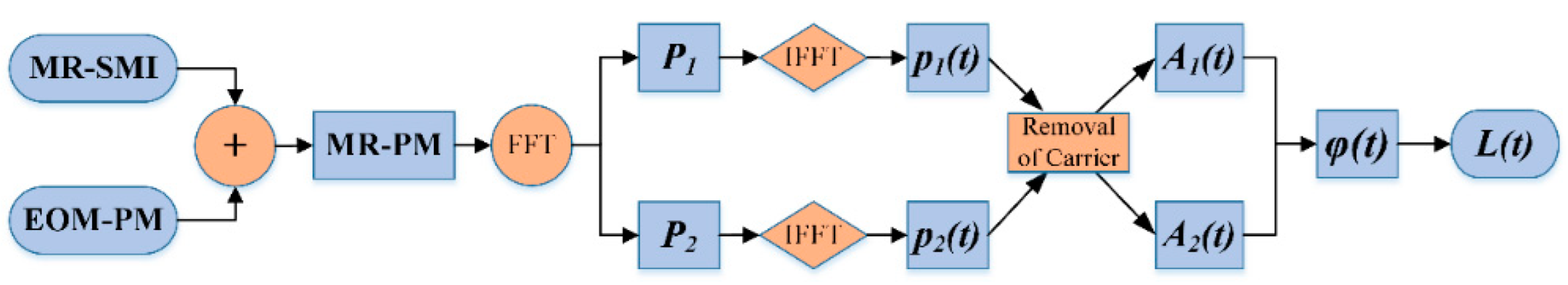
In this paper, we present an improved method to reconstruct the displacement of vibrating targets based on multiple reflection with the phase-modulation technique (MR-PM). First, sinusoidal phase modulation is performed by using an EOM placed in the external cavity. Then, the spectrum is obtained by Fourier transform of the modulated SMI signal. The wrapped phase is estimated by extracting the first and second harmonic from the spectrum. Lastly, through the phase-unwrapping process and simple mathematical calculation, the displacement of the target can be reconstructed. Owing to the application of multiple reflection technology, the method demonstrated has the advantage of reconstructing weak vibration far less than λ/2. Moreover, the method can obtain scalable fringe precision by increasing the reflection times, which makes it more competitive in the field of nanometer measurement.
2. Theoretical Analysis and Methods
In an SMI system, the wavelength and power of a laser beam will be modulated when the reflected or back-scattered light from the outer objective reenters the laser. On the basis of the three-mirror cavity theoretical model [
21,
22,
23], the emitted laser power
P is usually expressed as:
The interference phase is determined by the phase equation:
Equation (1) is the power equation of the SMI system, where
refers to laser power without laser feedback, and
refers to the modulation index. Equation (2) is the phase equation of the SMI, where
denotes the linewidth enhancement factor and
C denotes the optical feedback intensity factor.
denotes the phase signals of the laser without optical feedback. When the system stays in weak feedback regime
, the phase equation has only one solution, that is, the laser is in single-mode operation. At this time, the phase of the optical feedback changes slightly, which is approximately equal to the phase without optical feedback, that is:
where
represents the wavelength of laser,
represents the distance change from the laser diode (LD) to the target,
L0 represents the initial distance between the outer objective and the laser,
represents the displacement of the outer objective,
represents the initial phase of the self-mixing signal, and
represents the phase change caused by the displacement of the target.
The main principle of the multiple-reflection method is that an external mirror is placed in the optical path to increase the transmission of the optical path of the laser, thus improving the precision of the fringe. Through the analysis of the optical path after multiple reflection, the gain of optical path
can be obtained as [
12]:
where
is the reflection time and
is the laser beam incident angle. According to the in-depth analysis, the measurement error of the system can reach the minimum when
θ is 10°. Therefore,
θ is fixed to 10° in subsequent simulations and experiments. After the introduction of multiple reflectors in the SMI system, the feedback phase of the system is as follows:
where
represents the phase change caused by the displacement of the target object after multiple reflections.
In order to further improve the measurement accuracy of the system and realize the displacement reconstruction of the outer objective, we placed an EOM in the external cavity of the multiple-reflection self-mixing interference (MR-SMI) system. We ensured that the laser polarization direction was consistent with the main axis direction of the EOM, so that the EOM could produce a pure sinusoidal phase modulation on the laser output of the system. The phase-modulation function can be specifically expressed as:
, where
h is the modulation depth of EOM,
denotes the modulation frequency, and
denotes the initial phase of modulation. Since the laser traverses the EOM twice in the external cavity, the system phase change caused by EOM modulation should be
, so the power equation of the modulated MR-SMI signal can be expressed as:
We can further expand Equation (6) according to the Bessel function to obtain:
The first term in the formula is the DC component of the signal, and the second and third terms are the AC component of the signal. The AC component can be expanded into the form of
nth harmonics.
and
correspond to even-order and odd-order Bessel functions of the first kind, and their values are determined by the modulation depth
h of the EOM. Analyzing Equation (7), it can be concluded that the output power of the modulated MR-SMI signal is shown as a series of periodically changing signal superposition in the time domain. In the frequency domain, the frequency spectrum is mainly composed of the fundamental frequency component and the harmonic components distributed at integer multiples of
. According to the expansion formula, the first and second harmonic components of the output signal are, respectively:
where
and
are the amplitudes of the first harmonic component and the second harmonic component, respectively. It can be seen from the expressions of the two that
and
are modulated by the sine and cosine functions of the feedback phase of the system, and are related to the values of the first-order and second-order Bessel functions, respectively. Therefore, by dividing
and
, the required phase
can be demodulated. Finally, the displacement
L(t) of the vibrating target can be calculated. The specific calculation formula is as follows:
Based on the above analysis, the flow chart of multiple reflection combined with EOM phase modulation (EOM-PM) to achieve displacement reconstruction is shown in
Figure 1.
3. Results
Based on the theoretical analysis above, a series of simulations with different amplitudes and reflection times are conducted to prove the utility of the MR-PM method. The wavelength of LD is 532 nm with the feedback factor
and the linewidth enhancement factor
. The outer objective is set to have a sinusoidal waveform with an amplitude of
(
A =
) and a frequency of 200 Hz, as shown in
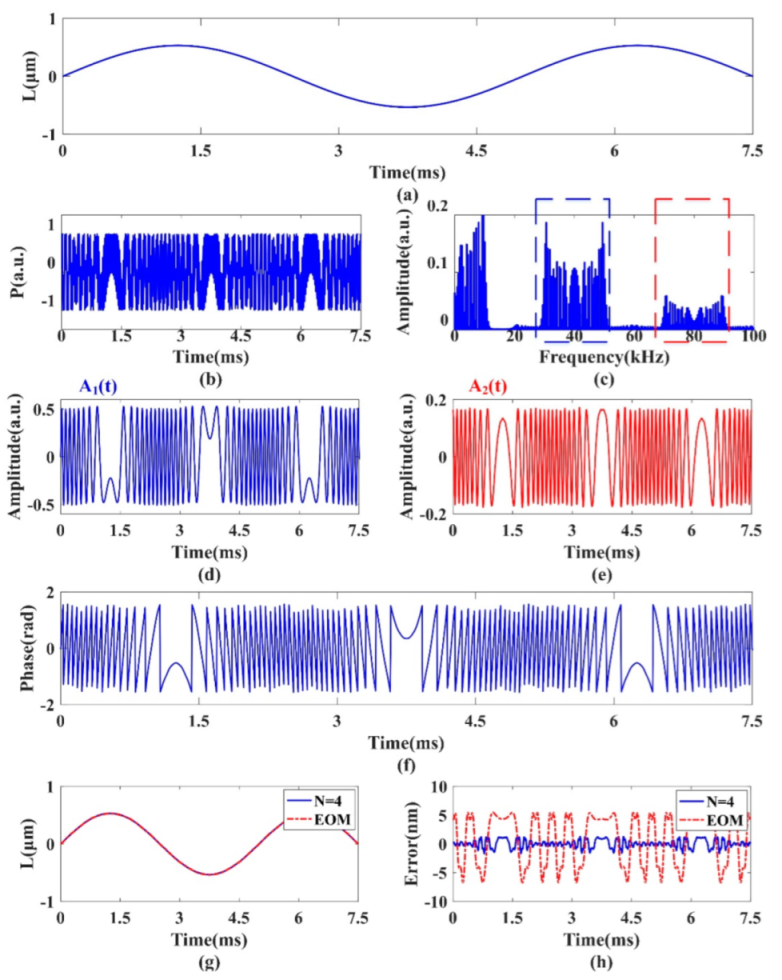
Figure 2a. The modulation depth of EOM is set to 1.2 rad, the modulation frequency is 40 kHz, and the initial phase of modulation is 0.
Figure 2 shows the specific realization process of the displacement reconstruction of the MR-PM method with
N = 4.
Figure 2b shows the phase-modulated SMI signal, which has a certain periodicity. After Fourier transform processing, the frequency spectrum obtained is shown in
Figure 2c. It can be intuitively seen that the harmonic component of the signal is mainly distributed at integer multiples of 40 kHz, which is consistent with the conclusion of theoretical deduction. The desired first harmonic (blue dashed line box) and second harmonic (red dashed line box) are extracted by a window with a specific range, and the other harmonic components are discarded, so as to achieve the purpose of noise suppression. After the inverse Fourier transform is carried out on the extracted spectrum, the time domain signals of the first and second harmonics are obtained respectively. After removal of the carrier, the amplitude
A1(
t) of the first harmonic can be obtained, as shown in
Figure 3d. The amplitude
A2(
t) of the second harmonic is obtained in a similar way, as illustrated in
Figure 2e. Substituting
A1(
t) and
A2(
t) into Equation (11) for calculation, the phase information of the outer objective can be obtained as shown in
Figure 2f. This phase is wrapped in the range −
/2~
/2. After a phase-unwrapping process, the reconstructed displacement with MR-PM method is displayed as the solid blue line in
Figure 2g. The red dotted line in
Figure 2g represents the reconstruction displacement with the EOM-PM method. As can be seen from
Figure 2h, the reconstruction error of MR-PM method is significantly smaller than that of EOM-PM method, which implies that the introduction of multiple reflections can reduce the reconstruction error.
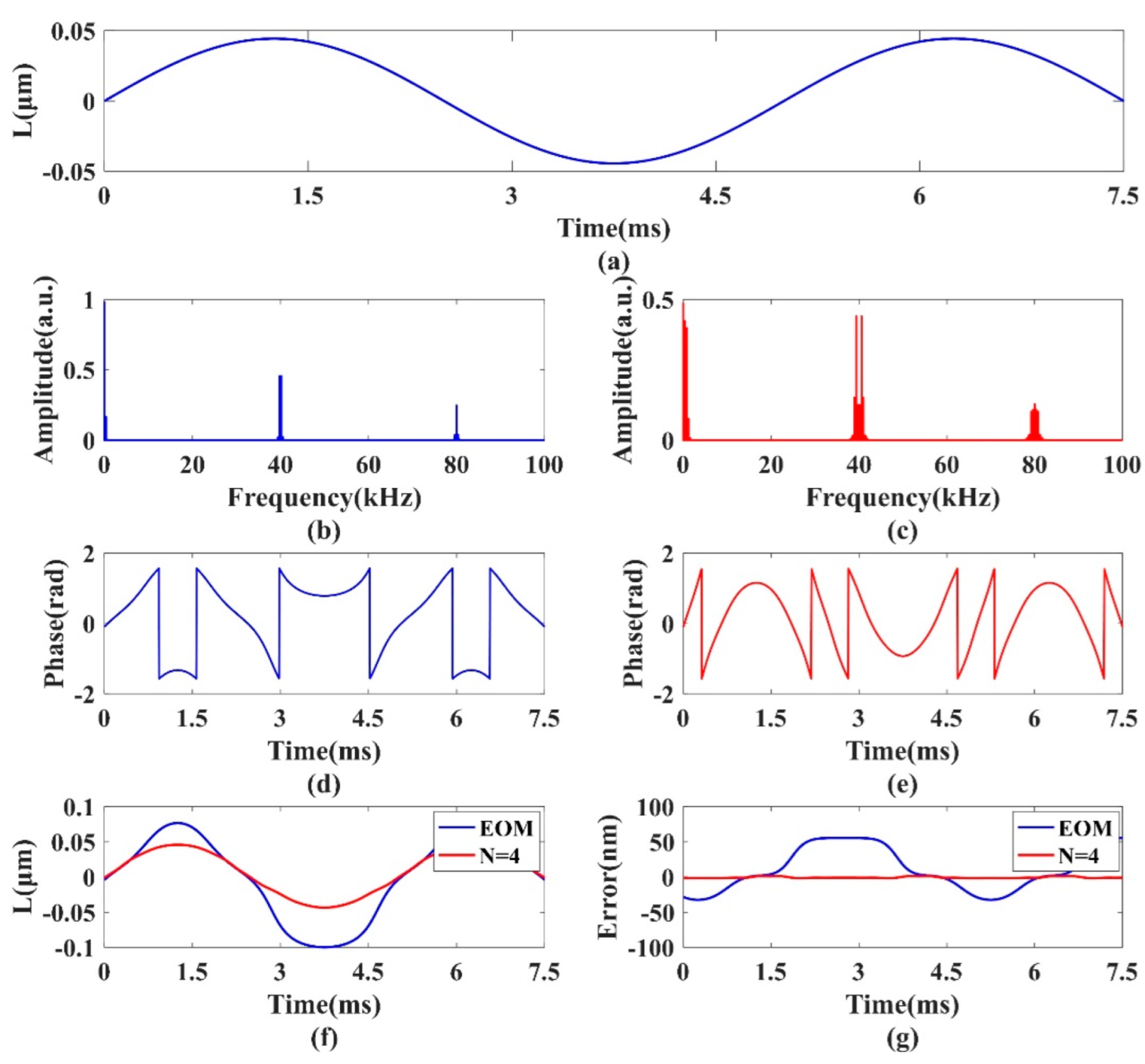
In order to demonstrate the advantages of the proposed MR-PM method, the simulation is conducted when the external vibration amplitude is decreased to
(
A =
) with other parameters remaining unchanged.
Figure 3a displays the simulated displacement of the outer objective.
Figure 3b displays the obtained SMI signal spectrum generated by the EOM-PM method. It is noticeable that the harmonic components are extremely narrow due to weak vibration, which results in the failure of the demodulation of the wrapped phase and the displacement reconstruction, as shown by the blue curve in
Figure 3d,f. In contrast, the spectrum of the harmonic components is significantly broadened by using the MR-PM method with
, as shown in
Figure 3c. The corresponding reconstructed displacement, denoted by the red curve in
Figure 3f, is basically consistent with the actual displacement. As can be seen from
Figure 3g, the reconstruction error of the MR-PM method (in red) is less than 2 nm, while the maximum reconstruction error of the EOM-PM method (in blue) is about 55 nm. Consequently, the weak vibrations far less than
can be successfully recovered by employing the MR-PM method.
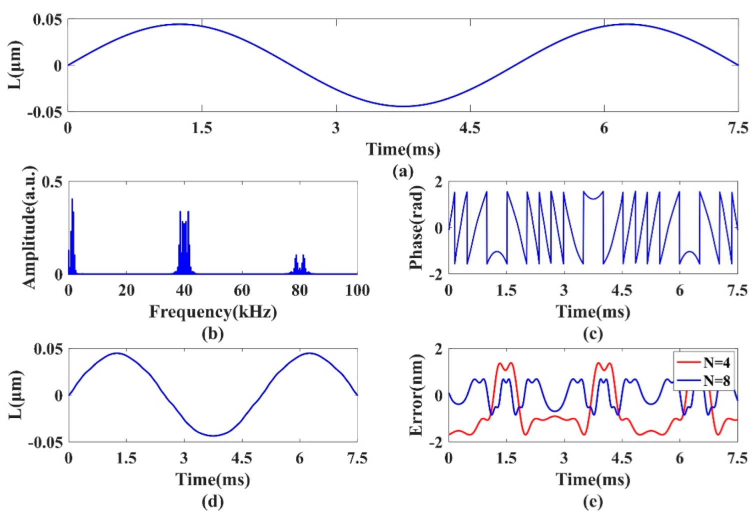
To illustrate the effect of the reflection time
N on the reconstruction error of the MR-PM method, the reflection time
N is increased to 8 while the other parameters remain unchanged, as shown in
Figure 3. The simulation results are shown in
Figure 4.
Figure 4b–d present the signal frequency spectrum, the wrapped phase and the reconstructed displacement, respectively. Compared with the result of
, it can be found that as reflection times increase, the harmonic components of the signal spectrum broaden, and the number of fringes in the wrapped phase increases. As a result, the system will obtain higher measurement accuracy. As can be seen from
Figure 4e, the reconstruction error with
(in blue) is further reduced compared with
(in red). Nevertheless, according to Nyquist’s law, the sampling frequency should satisfy the equation:
where
denotes vibration frequency and
denotes amplitude of the target. Combining the two equations, the sampling frequency is limited to:
which means our measurement range of the frequency and vibration amplitude of the target will be confined due to the lack of sampling frequency.
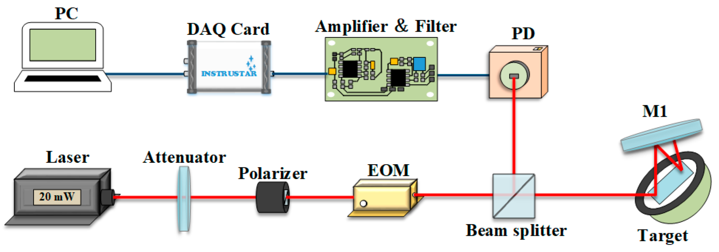
The experimental arrangement is displayed in
Figure 5. The light source adopted an all-solid-state pumped laser (MGL-III-532-20mW) with a wavelength of 532 nm and output power of 20 mW. A variable attenuator (VA) is placed next to front facet of laser to adjust the intensity of reflected light into the laser, which ensures the system under a weak feedback regime. The EOM (New Focus, 4002), which is placed in the external cavity, modulates the light with a sinusoidal phase. Considering that only polarized light can be phase modulated, a polarizer is placed in front of the EOM to generate polarized light. The target (speaker), with a mirror attached to its surface, is placed on an optical adjustment stage and is driven by a signal generator (AFG3022). To confirm the exactness of the strategy, a business interferometer (LV-IS01, SOPTOP) with a precision of around 0.15 nm is utilized to measure the displacement of the same object for comparison. The external mirror M
1 is placed at the distance of 2 cm from the target, and is changed cautiously to accomplish multiple reflections as the collimated beam reentered the laser. The changes in laser output power are distinguished by a power-monitor PD (PDA10A2) and changed into current, which are processed by the amplifier and filter circuit. Ultimately, the data are gathered by a PC through a data-acquisition card (DAQ card) (ISDS205A).
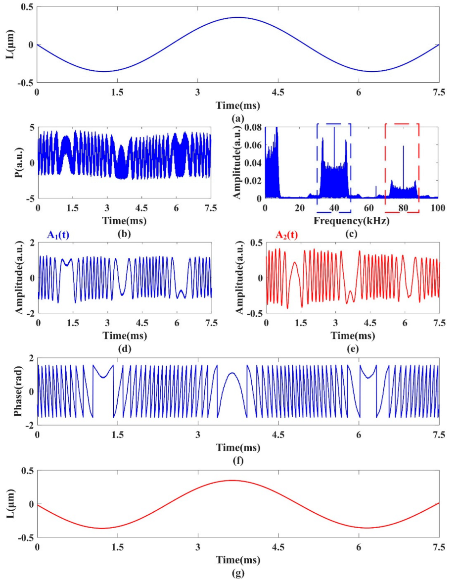
First, the signal generator provides a sinusoidal motivation with a driving voltage of 0.8 V (the corresponding amplitude
A = 356 nm) and frequency 200 Hz to drive the target (speaker), as shown in
Figure 6a. The external mirror M
1 is adjusted to make the laser beam reflect four times, i.e.,
N = 4. The modulation voltage and frequency of EOM are set to 6.75 V and 40 kHz, respectively. The specific process of displacement reconstruction using the proposed MR-PM method is shown in
Figure 6.
Figure 6b shows the SMI signal with EOM phase modulation.
Figure 6b clearly shows that a number of modulation peaks appear on the SMI signal peak with the addition of modulation. The spectrum illustrated in
Figure 6c is obtained after Fourier transform of the modulated signal, in which the harmonic components are concentrated at integer multiples of 40 kHz. The first and second harmonics are extracted by two filters in the frequency domain, and the amplitudes
A1 and
A2 of the first and second harmonics are obtained after inverse Fourier transform and carrier removal, respectively, as shown in
Figure 6d,e. Due to the interference during the experiment,
A1 and
A2 show obvious fluctuations. However, the influence of signal intensity fluctuations is offset by dividing the two, which obtains a relatively flat wrapped phase as shown in
Figure 6f. After unwrapping the phase and using Equation (12), the vibration displacement of the target is reconstructed in
Figure 6g, which basically coincides with real displacement. In this case, the maximum reconstruction error is 4.7 nm.
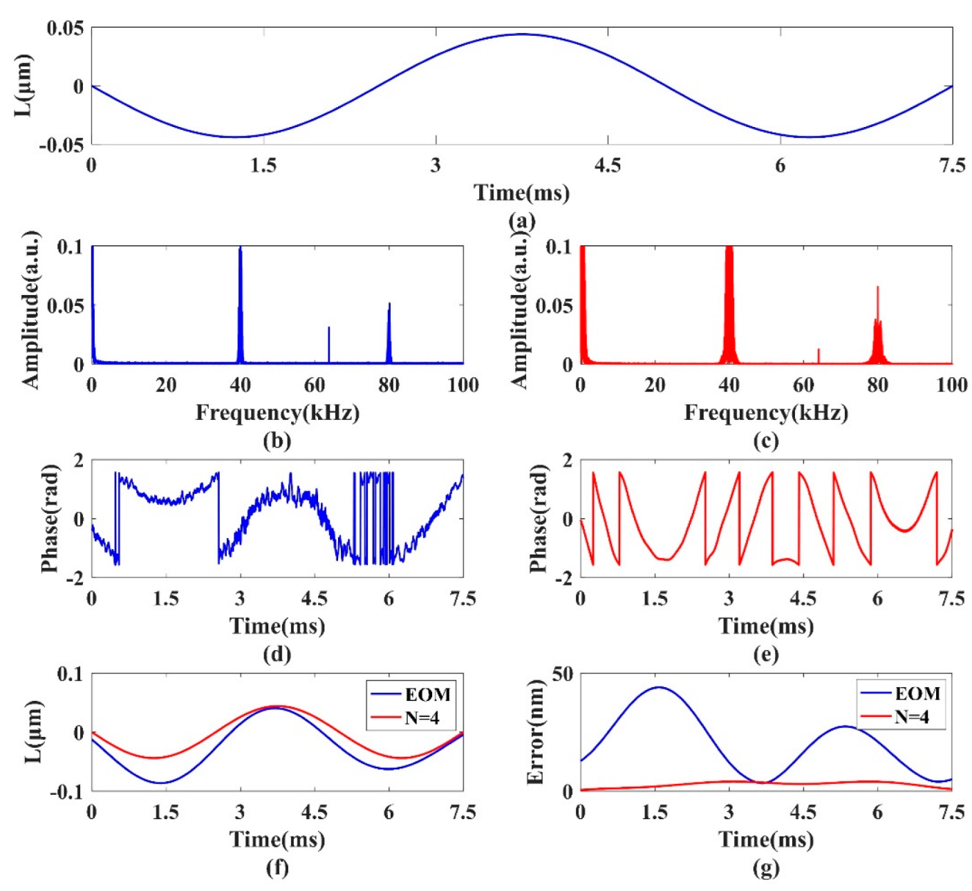
To additionally outline the predominance of the proposed MR-PM technique, the comparative experiments are conducted by utilizing the conventional EOM phase modulation (EOM-PM) method. The driving voltage of the target is reduced to 0.1 V (the corresponding amplitude
A = 44 nm) while other parameters are the same as given in
Figure 6.
Figure 7b shows the SMI signal spectrum produced by the EOM-PM method. It can be seen that the harmonic component is extremely narrow due to the weak vibration, which results in a larger distortion of the wrapped phase shown in
Figure 7d. Correspondingly, the reconstructed displacement deviates greatly from the real displacement, as shown in
Figure 7f.
Figure 7c shows the SMI signal spectrum of the proposed MR-PM method with
N = 4. It is demonstrated that the spectrum of harmonic components is essentially broadened because of multiple reflections. Consequently, this method will facilitate the accurate estimation of the wrapped phase and the realization of displacement reconstruction, as shown in
Figure 7e,f. As can be seen from
Figure 7g, the reconstruction error of the MR-PM method is within 5 nm, while that of the EOM-PM method is up to 44 nm.
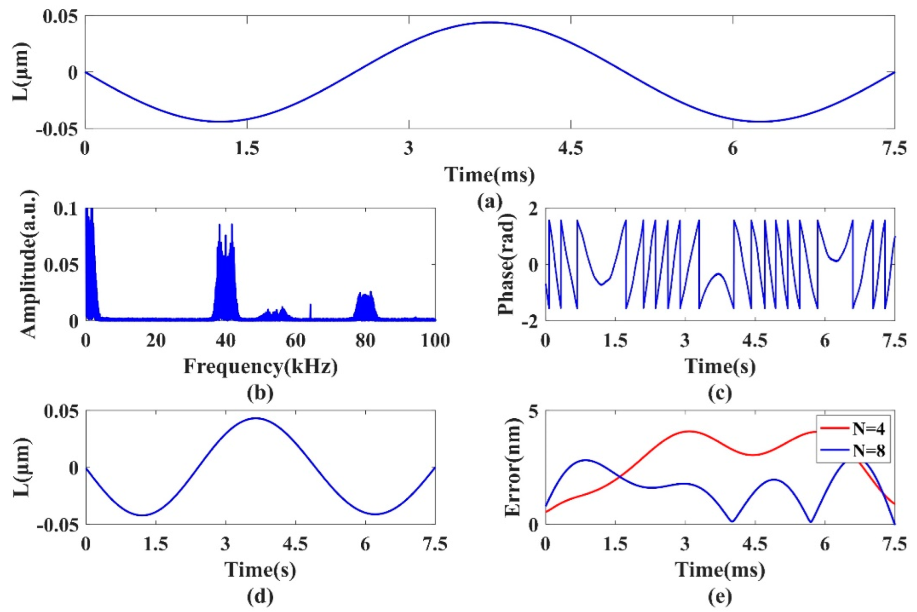
To verify the influence of reflection time N on the displacement reconstruction error of the MR-PM method, an experimental comparison of
N = 4 and
N = 8 is performed with the parameter settings in
Figure 7. The specific experimental results are illustrated in
Figure 8.
Figure 8b–d shows the signal frequency spectrum, the wrapped phase, and the reconstructed displacement with
N = 8, respectively. Compared with the experimental results of
N = 4 in
Figure 7, it is obvious that that the increase in reflection time N results in a broader spectrum of the harmonic components and a larger number of fringes in the wrapped phase; thus, the reconstruction accuracy is higher. As can be seen from
Figure 8e, the maximum reconstruction error of
N = 8 is less than 3 nm. Further experiments demonstrate that the measurement accuracy of MR-PM method is scalable with the increase in
N.
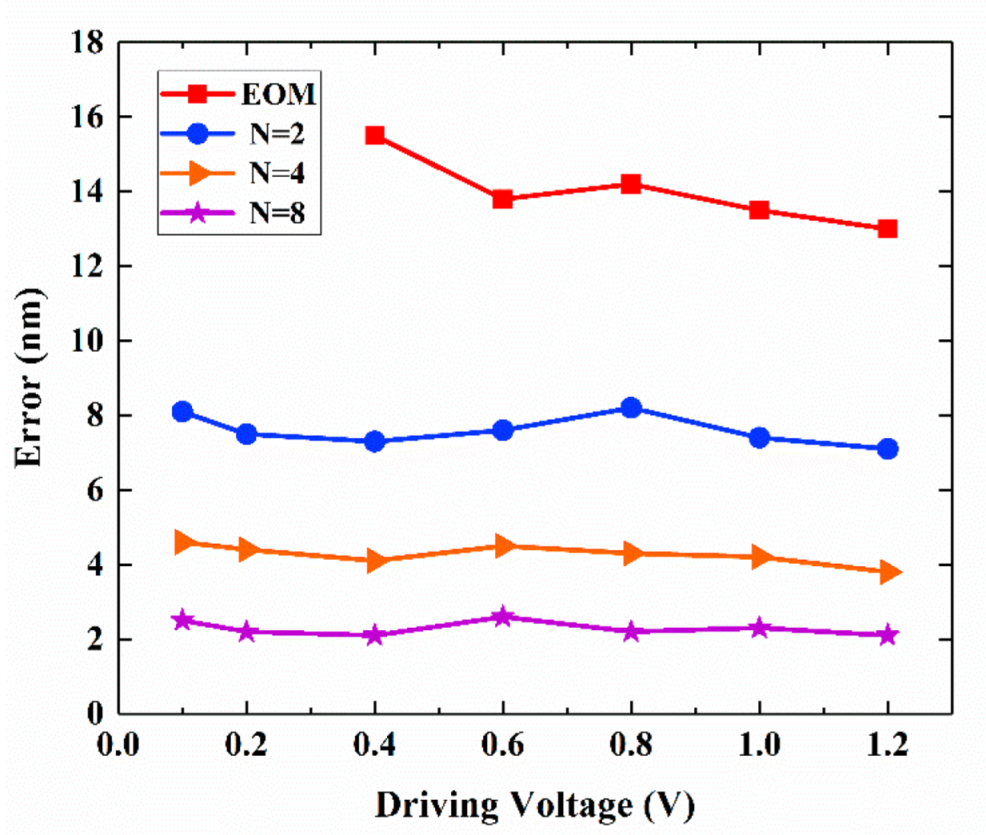
In addition, experiments with various vibration amplitudes are performed to confirm the superiority of the MR-PM method. The driving voltage of the target varies from 0.1 V to 1.2 V, and other parameters are kept the same as those in the previous experiment. The reconstruction errors of the proposed MR-PM method with different reflection times N and the EOM-PM method are illustrated in
Figure 9, respectively. When the driving voltage is 0.4 V to 1.2 V, the reconstruction error of the EOM-PM method is between 12 and 16 nm. However, for the cases of the driving voltages 0.1 V and 0.2 V, the reconstruction errors both exceed 40 nm, which indicates that the EOM-PM method is invalid. In
Figure 9, the reconstruction error of the MR-PM method decreases with the increase in reflection times N, and is always better than that of the EOM-PM method. When
N = 8, the reconstruction errors are all less than 3 nm with different vibration amplitudes.


