1. Introduction
There has been a recent and rapid development of three-dimensional (3D) laser scanning technology for use in reverse engineering, digital cities, deformation monitoring, and other applications [
1]. Owing to limitations in the field of view of 3D laser scanning equipment, and the complex geometry of the scanned objects themselves, the point cloud data collected from each viewpoint only partially cover the geometric information of the scanned object surfaces. To obtain complete information regarding such surfaces, it is necessary to register the point clouds from individual scans into the same reference coordinate system.
To date, the classic iterative nearest point (ICP) [
2] remains the most widely-used point cloud matching algorithm. Many researchers have made improvements to the ICP algorithm [
3,
4,
5,
6], which relies on a good initial alignment position. Without this, it quickly falls into the local optimum and cannot achieve a good registration effect. Therefore, as common practice, the initial alignment method is used to obtain a good initial alignment position and then the ICP algorithm is applied to achieve an accurate alignment. Due to the irregular nature of 3D point clouds, designing a local surface descriptor with high overall performance is a challenge. Three-dimensional point cloud descriptors fall into two main categories: handcrafted and deep learning based methods. The incredible power of deep learning techniques has resulted in a breakthrough in the obtainment of 3D point cloud descriptors. As an example, Deng et al. [
7] proposed the Point Pair Feature NETwork, which uses a new N-tuple loss and an architecture that naturally injects global information into the local descriptors, achieving good results in terms of accuracy, speed, and other factors. In addition, Ao et al. [
8] proposed Spinnet, which first introduces a spatial point transformer to map the input local surface into a well-designed cylindrical space and then applies a powerful point-based and 3D cylindrical convolutional neural layer feature extractor to derive compact and representative descriptors for matching. Spinnet has an excellent ability to generalize well under unseen scenarios. Finally, Fabio et al. [
9] normalized their estimated local reference system by extracting point cloud patches and encoding rotationally invariant compact descriptors using a robust deep neural network based on PointNet. Although deep learning has made significant progress in the area of point cloud alignment, it inherently requires a large amount of training data, and a separate training process is needed to learn a separate feature extraction network, which is time-consuming and results in significant hardware requirements.
For handcrafted methods, such descriptors are divided into two categories depending on whether a local reference frame (LRF) is used. Although many efficient methods have been proposed for descriptors without an LRF, point pair feature (PPF) based descriptors are the most classical approaches for a 3D surface description. Johnson and Heber [
10] proposed using spin image (SI) features, in which the normal vectors of the key points are first applied as reference axes and the local neighborhood points are then projected onto a 2D surface both horizontally and vertically. Although an SI is a frequently cited descriptor, it has limited descriptive power and is sensitive to changes in the data resolution. In addition, a point feature histogram (PFH) [
11] has high discriminatory power but is extremely time-consuming. To address this problem, Rusu et al. [
12] constructed a fast point feature histogram (FPFH) using a simplified point feature histogram (SPFH), which is characterized as fast and discriminative. Albarelli et al. [
13] defined a descriptor for low-dimensional surface hashing and applied it to the surface matching problem in a game-theoretic framework, where the surface hash features are mainly computed based on multiscale statistical histograms of the local properties, including normal vector pinch angles, integral volumes, and their combination. Moreover, Zhao et al. [
14] proposed a novel normal surface reorientation drawing upon a Poisson-disc sampling strategy to address the problem of data redundancy during data preprocessing. Subsequently, a new technique is used to divide the local point pairs for each key point into eight regions, where each local point pair distribution region is applied to construct the corresponding sub-features. Finally, an extracted histogram of the point pair features is generated by concatenating all the subfeatures into a single vector.
For LRF-based features, Stein and Medioni [
15] designed the local characteristics of point clouds as a consequence of the offset angle, torsion angle, and curvature relationships between key points and those within the geodetic neighborhood. Frome et al. [
16] also suggested using a 3D shape context (3DSC) by extending the 2D shape context (SC) [
17] into the 3D domain. The proposed method first divides the local spherical domain into multiple subspaces and then computes the feature descriptors by calculating the percentage of points in each subspace. Zaharescu et al. [
18] compute gradient vectors for each neighborhood point and project them onto three orthogonal planes of the LRF. Each plane is divided into four quadrants, and each quadrant corresponds to an 8-dimensional feature. In addition, Prakhya et al. [
19] form a histogram by accumulating the points in each interval divided by a “3D” descriptor. As a concrete process, the local surface of the key points is aligned to the defined LRF by employing a “3D” descriptor, and the range between the minimum and maximum x-coordinate values of the points on the surface is then divided into D intervals along the x-axis. The same process is repeated along the y- and z-axes, and a 3D histogram of the point distribution (3DHoPD) is generated by concatenating these histograms. Although this method is fast, it is poorly descriptive. Guo et al. [
20] first rotate the local surface in the LRF, project the surface after each rotation to calculate the projected point density statistics, and concatenate these statistics to obtain rotational projection statistics (RoPs). Although the use of RoPS has achieved the highest matching performance for several datasets, its shortcomings include a poor descriptiveness and time-consuming computations for data with uneven point distributions. Similar to the rotational projection mechanism of RoPS, Guo et al. [
21] use the three orthogonal axes of the LRF to compute three spin map features and obtain triple spin images (TriSI) that are more resistant to occlusions than RoPS but are still more time-consuming.
In this paper, a point cloud alignment algorithm based on the 3D point neighborhood feature histogram (3DNPFH) descriptor is proposed to address the current problems inherent to an alignment algorithm. After uniform sampling using the voxel grid method, the algorithm transfers the key points to the new 3D coordinate system for the point cloud. The point pairs to be matched are obtained using the principle in which the key points are generated by similar numbers of 3D surfaces that are close to each other. We construct the neighborhood point feature histogram (NPFH) descriptor by calculating the normal vector, curvature, and distance features within the neighborhood of the key points, and finally apply the RANSAC algorithm to achieve a coarse alignment and obtain a good initial alignment position.
2. Proposed Methods
In general, in a 3D surface description, a unique high-dimensional feature vector is used to describe a local 3D surface at a 3D key point. In this study, a 3D neighborhood point feature histogram (3DNPFH) is proposed to represent a local 3D surface. Generating the 3DNPFH descriptor involves two main steps: encoding the 3D key point positions to form a pre-3D descriptor and obtain a list to be matched, and finding an exact match by computing the NPFH descriptor. Let us consider an input source point cloud upon which key points, , where , are extracted using a uniform sampling. We then create a 3DNPFH descriptor from its radius neighborhood surface, , including K points, where . The neighborhood surface from which the descriptor is constructed is determined based on its support radius r. A key point has , where represents the index of the key points, and k represents the index of the points within the surface of the neighborhood of the key points.
2.1. Encoding 3D Key Point Locations
The uniformly-sampled key points are transformed into a new 3D coordinate system, and their 3D coordinates are recorded in the first three dimensions of the 3DNPFH descriptor. The extraction of feature descriptors around the key points and a comparison to find their correspondences are conducted to locate exact 3D key point correspondences generated from a similar 3D surface neighborhood. Therefore, the key points are transformed into a new 3D coordinate system in which the key points of similar surfaces are close to one another. We first calculate the centroid coordinates
in the neighborhood coordinate system
of surface radius
r of key point
, and then subtract the centroid coordinates
from all point coordinates in
, effectively generating a new surface
, and letting the key points
subtract the centroid coordinate
to obtain
. Finally, we have a new surface,
, used to calculate the local reference coordinate system {a}. The three axes of {a} form the rotation matrix
, and the key point
is then transferred to a new 3D coordinate system, as shown in (1).
where its new coordinates,
, constitute the first three dimensions of the descriptors proposed herein.
Local reference coordinate system: This algorithm establishes a local reference frame, such as SHOT [
22], and the corrected covariance matrix of the point cloud is then calculated using the 3D surface
, as shown in (2). Within the radius neighborhood of the considered key points, weighting is conducted according to the distance
of the key points from the centroid. For better readability, we use
to represent the point within the surface
around the key points, and q to represent the distance between the key points and the centroid
.
Here,
. To create a unique local reference coordinate system, it is necessary to disambiguate the direction of the normal. We use the orientation of the local x- and z-axes toward the principal directions of the vectors they represent, and finally obtain the local y-axis through the cross product of z and x, where y = z × x. By solving the covariance matrix COV, we can obtain the eigenvalues and the eigenvectors corresponding to the eigenvalues, which can be sorted in descending order to obtain
. The corresponding eigenvectors x, y, and z represent the three coordinate axes, and the rotation matrix is constructed as follows:
However, because there may be various anomalies, we cannot state that the point closest to the key point in the new 3D coordinate system is the correct match; for example, noisy point cloud data may be acquired by the sensor or similar local reference coordinate systems. However, the correct match lies within the neighborhood of the key points, significantly reducing the search coordinate system for correctly matched points.
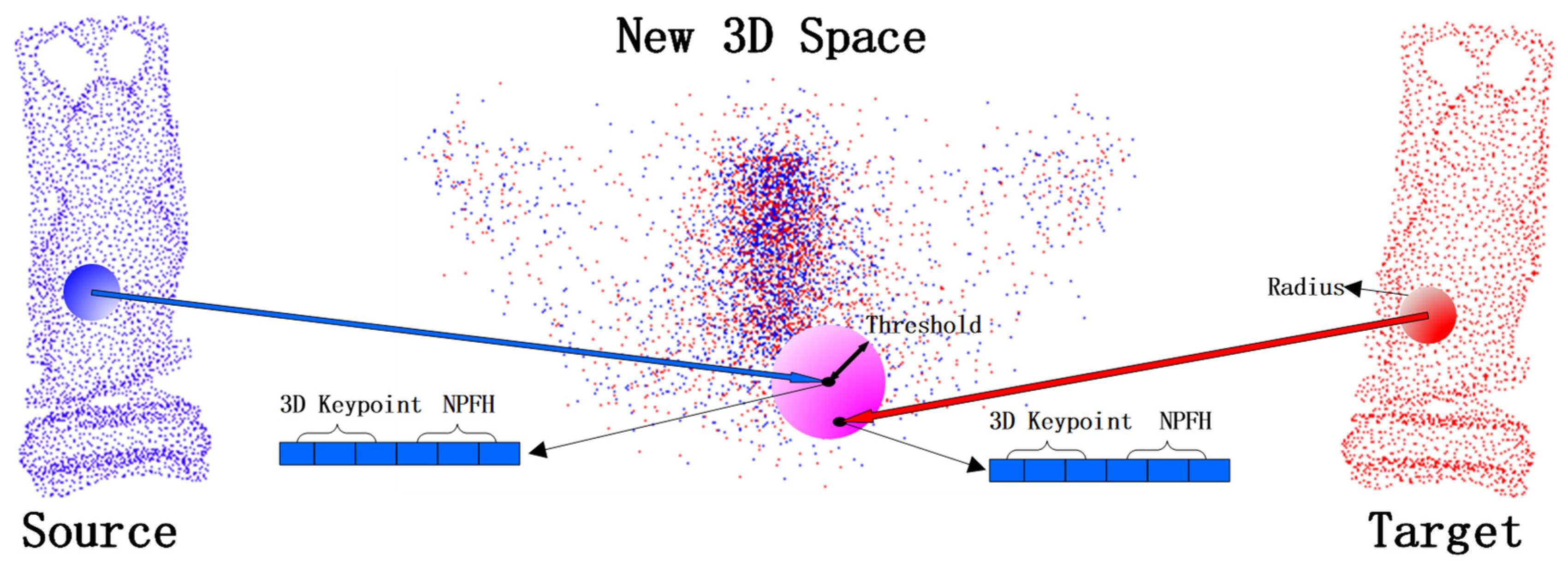
Figure 1 shows a schematic of the 3DNPFH descriptor. The key points of the source point cloud are shown in blue, and the key points of the target point cloud are shown in red. The blue and red spheres represent the LRF and the support size of the constructed descriptor, respectively. Then, for each model key point, the list of key points in the scene (shown as pink spheres in the new 3D coordinate system) is retrieved through a radial search of the threshold radius. From this retrieved list of possible key point matches of a scene, the one closest to the NPFH descriptor is considered an exact match.
2.2. Calculation of Neighborhood Point Feature Histogram (NPFH)
Geometric features such as the curvature, surface normals, and distances reflect the most basic geometry of a point cloud, which is the key to expressing the local features of the cloud. In this section, based on the radius neighborhood of the key point, the neighborhood curvature sum, normal vector angle sum, and distance sum corresponding to the key point are calculated. A 3D vector consists of the sum of the curvature of the neighborhood, the sum of the angle between the normal vectors, and the sum of the distance. This 3D vector is an NPFH descriptor.
2.2.1. Curvature
The normal and curvature information of a point cloud surface are important geometric features for 3D object recognition. The curvature is invariant to rotation, translation, and scaling and is therefore used as a feature element. The curvature value reflects the degree of concavity of the point-cloud surface. The sharp features of the point cloud have a more significant curvature. By contrast, the non-featured parts of the point cloud exhibit a relatively slight curvature.
In this study, the method described in [
23] is used to estimate the norm and curvature of the data points by analyzing the covariance of
k neighborhood points within radius
r. We analyze the covariance of a given point of the neighborhood point covariance for point cloud datasets and solve the covariance matrix. The direction of the eigenvector corresponding to the smallest eigenvalue is defined as the normal value of the point. The curvature of the point is then estimated based on the surface variation of the point in the local area. The curvature
is calculated as follows:
First, the following is calculated:
This is transformed into solving the eigenvalues and eigenvectors of matrix
, where matrix
is a covariance matrix of
k points, and (
,
,
) are the eigenvectors of the matrix. Each data point
in the point cloud corresponds to matrix
as follows:
where
is a positive semi-definite third-order symmetric matrix,
is the centroid of the point within the neighborhood of the key points
, and
is the coordinate of the point in the radius neighborhood of
. The three eigenvalues
,
, and
of matrix
and the corresponding unit eigenvectors
,
Assuming that
≤
≤
,
describes the change in the surface in the normal direction and represents the distribution of data points on the tangent plane, the curvature can then be expressed as
2.2.2. Deviation Angle between Normals
Previous studies have demonstrated that a representation based on the deviation angle between two normals has a high discriminative power [
9]. The normal directions of
and
are
and
, respectively. The cosine of the normal angle between
and
can be expressed as
The sum of the angles normal to the key points and all points in the radius neighborhood is calculated as follows:
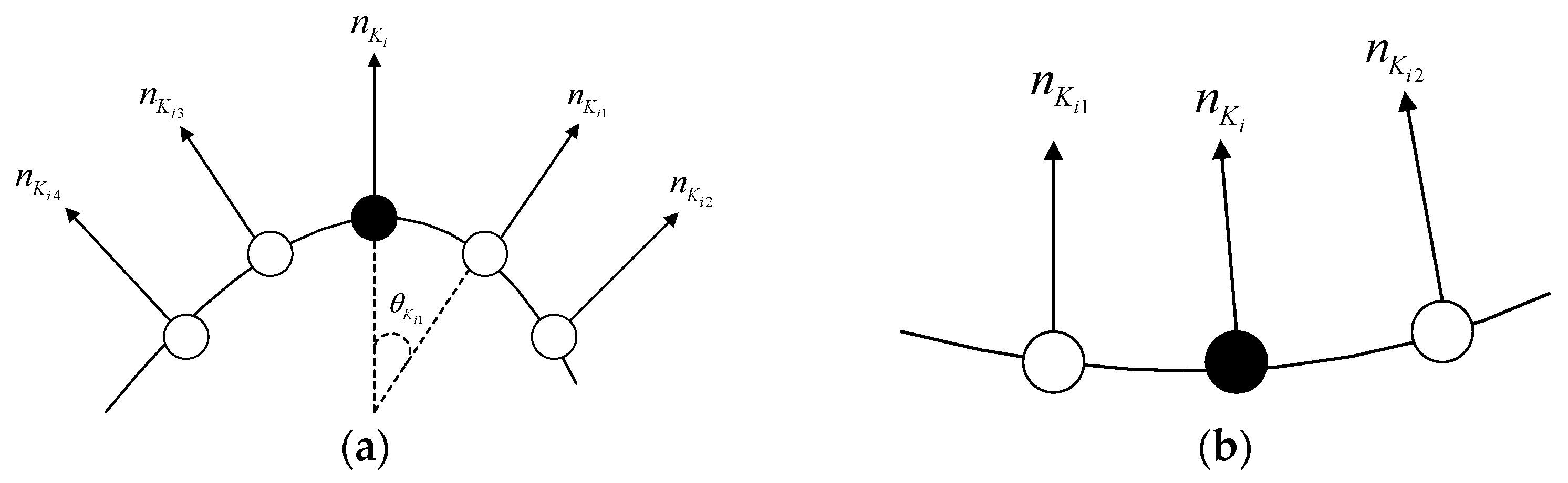
Figure 2 shows a schematic of the angle between the normal vector of the feature and non-feature regions. In
Figure 2a, the normal angle in the neighborhood of the key point
is larger, which generally forms the feature region of the point cloud. In
Figure 2b, the normal angle within the neighborhood of key point
is smaller, which generally forms the non-featured region of the point cloud. Therefore, the normal vector angle is also used as a parameter to calculate the feature description of the point cloud.
2.2.3. Sum of Distances between Neighborhood Points
For the radius neighborhood of a key point, the number of points within the neighborhood generally differs; therefore, the local 3D geometric features can be described by the distance sum of the neighborhood points.
The sum of the distances between the key points and the neighboring points reflects the characteristics of the point cloud. The point cloud feature is distinguished using the sum of the distances between the key points and neighboring points as the distance parameter.
The distance from a point in the neighborhood to a point in the radius neighborhood can be expressed using the following formula:
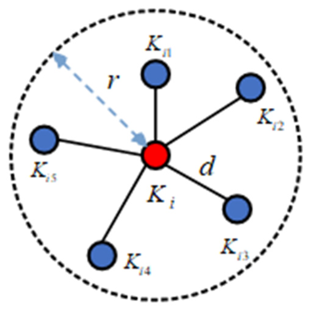
Figure 3 shows a diagram of the neighborhood point distances, where
is the key point, and
is the point within the radius neighborhood of
.
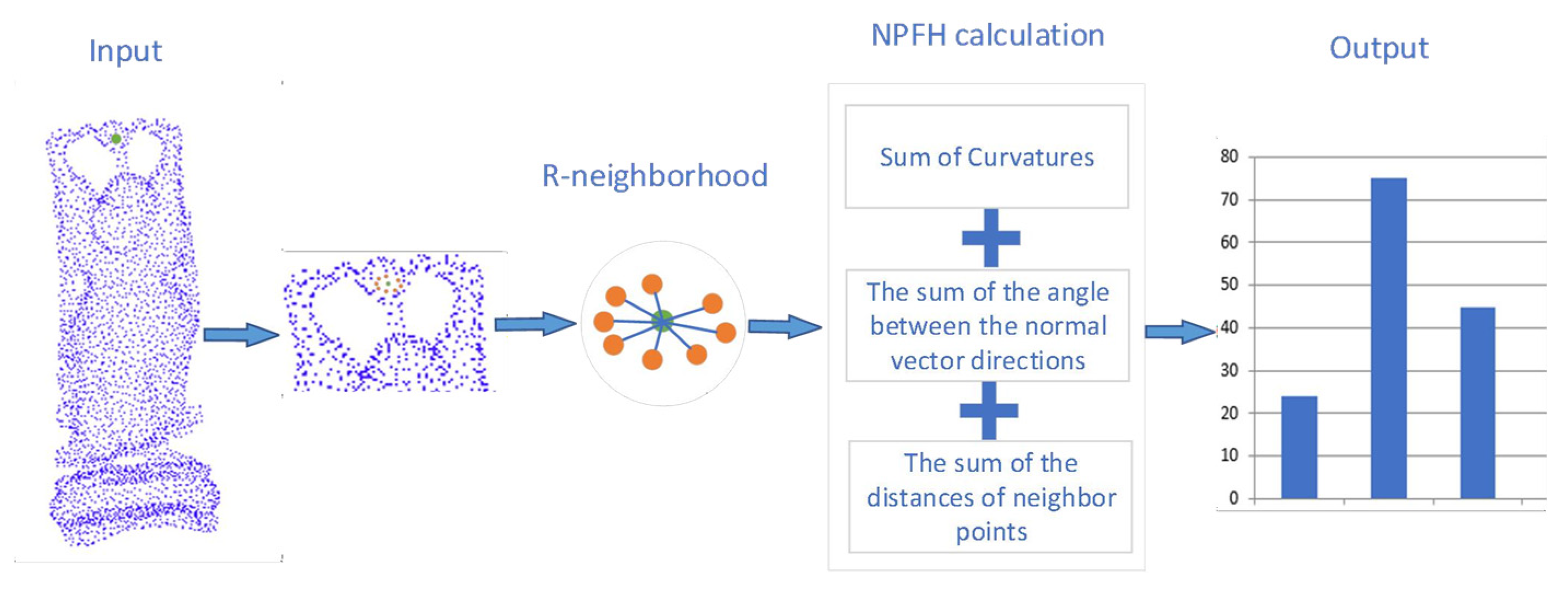
After proposing three local geometric features, three sub-histograms are obtained: the sum of the distances between neighborhood points, the sum of the curvatures, and the sum of angles between the normal direction of the key point and the normal direction of the neighborhood points.
Figure 4 shows a schematic of the NPFH feature-description mechanism. A 3DNPFH descriptor is created by combining the three sub-histograms above into a single histogram. The following are the three primary characteristics of the NPFH descriptor: The NPFH descriptor is computationally efficient, the three local geometric characteristics of the NPFH descriptor are low-dimensional and computationally efficient, and the computational cost of the NPFH descriptor is O(k), where k is the number of points within the radius neighborhood of key point
.
2.3. Matching
Taking advantage of the fact that key points generated by similar 3D surfaces are close to each other in the new 3D coordinate system, we apply the following matching of the 3DNPFH descriptors. First, the extracted key points are transformed into a new 3D coordinate system by constructing local reference coordinate systems for the key point neighborhood surfaces in the source and target point clouds. Then, for each source key point in the new 3D coordinate system, we find a list of the closest target key points in the new system that lie within the radius threshold . Finally, we find the most accurate nearest neighbors in the 3DNPFH descriptor using a Euclidean distance search to form the corresponding point pairs in the to-be-matched list.
2.4. Mismatch Rejection of RANSAC
The corresponding point pairs are identified using the 3DNPFH feature-based descriptors. This study uses the RANSAC algorithm to eliminate mismatched pairs and improve the alignment accuracy of two-point clouds. Assuming that n matching pairs are obtained after the above feature matching, the RANSAC algorithm is used to reject false matches and obtain the transformation relationships between the point clouds as follows:
Step 1: Randomly select three non-collinear points from the source point cloud P, denoted as , and search for their corresponding points from the target point cloud Q, which are denoted as , , and , as samples.
Step 2: Use the samples to estimate the rigid body transformation matrix .
Step 3: Using the model estimation matrix, transform the remaining points in the source point cloud and calculate the distance error between all points in the transformed source point cloud and the target point cloud if the distance error of one point pair is below the set threshold. If there is an error, the point is added to the interior point set ; otherwise, it is an outlier.
Step 4: Repeat the above process until the number of points in the interior point set reaches the set threshold or the iteration number becomes greater than the maximum iteration number, and then stop the iterative calculations.
Step 5: Select the model parameter with the most significant number of interior points in the interior point set as the optimal model parameter and use the optimal model parameter to achieve a rough registration of the point cloud.
Because of the increased proportion of correct points in the set of correspondence points optimized using the RANSAC algorithm, the resulting rigid body transformation matrix is more accurate and effectively reduces the error in the point cloud alignment. However, RANSAC requires multiple iterations in the algorithm, and thus a lengthy time is required to obtain optimal results when the number of correspondence point pairs is large. Therefore, when using the RANSAC algorithm, care should be taken to set the threshold error and the number of iterations, as reasonable settings can help improve the rejection of erroneous point pairs.


