1. Introduction
Optical vortices (OVs) are actively studied nowadays [
1,
2,
3,
4,
5]. For example, in [
1], the authors numerically simulated generation of an OV at near infrared wavelengths from an amorphous silicon photonic crystal slab. Conditions for the violation of the spiral beam structural stability influenced by sector perturbations were studied in [
2] using computer simulation and measurement of a mode spectra. In [
4], the authors investigated the propagation of Airy, cos-Airy, and cosh-Airy beam with OV in a strong nonlinear system using a Fourier transform. Of great interest are cylindrical vector beams (CVB) [
6,
7,
8,
9] and beams with a fractional topological charge [
10,
11,
12,
13]. In [
6], cylindrical vector spatiotemporal optical vortices were experimentally studied. In [
7], we theoretically and experimentally investigated an effect of a reverse energy flow at the focus of a second-order CVB which passed through amplitude zone plate. Conversion of linear-circular polarizations and spin-orbital angular momentums in a focused vector vortex beam with fractional topological charges were theoretically and numerically studied in [
10]. Properties of the focal spot and energy fluxes at the focus of fractional vector beams were considered in [
11]. In [
14], an optical setup was proposed for generating of a 2D optical vortex lattice. In [
15], a 3D optical vortex lattice was generated experimentally. Papers [
16,
17,
18] were devoted to the application of OVs for trapping and rotating microscopic particles. Another promising area for the use of OVs is optical communications and secure data transmission [
19,
20]. The paper [
21] investigated optical vortices in nanophotonics. OVs in structured waveguides were studied in [
22]. In [
23], distortions of spiral vortex beams were considered and such beams were demonstrated to be almost insensitive to the distortions.
For the majority of familiar optical vortices, the orbital angular momentum (OAM) (normalized to the beam power) and the topological charge (TC) are equal to each other. This is the case for Laguerre–Gaussian beams [
24], Bessel modes [
25] and Bessel–Gaussian beams [
26], Gaussian optical vortices [
27], hypergeometric modes [
28] and beams [
29], circular beams [
30], elliptical beams [
31], and many other well-known vortex beams. Meanwhile, the OAM and the TC of beams without cylindrical symmetry, for instance, asymmetric Bessel beams [
32] or Hermite–Gaussian vortex modes [
33], typically have different values.
Coaxial superpositions of OVs can also have different values [
34] of the TC and the normalized OAM. The OAM can have both an integer and a fractional value [
18], which conserves during propagation. If the TC is fractional in the initial plane, it becomes integer during propagation. Therefore, it becomes indefinite [
35] because it is not clear whether the fractional number should be rounded off to the nearest greater or smaller integer. In addition, if a single Gaussian OV has a half-integer TC in the initial plane, for instance,
n + 1/2, then during propagation, the TC becomes integer but undefined, since at different distances from the optical axis, the TC is either
n or
n + 1. In the case of a coaxial superposition of two Gaussian OVs, if the TC is half-integer ((
n +
m)/2) in the initial plane, then the TC becomes integer and equal to max(
n,
m) and conserves during propagation of such a vortex field [
34].
However, it is not difficult to obtain the TC of simple OVs [
4,
24,
25,
26,
27,
28,
29,
30,
31,
32,
33], and it is an unsolved problem for a superposition of OVs [
34]. For instance, the TC of the Laguerre–Gaussian beams superposition is equal to the maximal azimuthal number of the constituent Laguerre–Gaussian beams [
34]. The TC of a superposition of other-type OVs was not yet studied. The problem of obtaining the TC of an arbitrary OVs superposition is yet unsolved. Here, we consider a special case when coefficients and topological charges in the superposition are chosen so that they constitute a geometric progression. The problem of obtaining the TC of OVs superposition is highly related with the problem of OAM-sorting [
36]. If the OAM-spectrum of a composite vortex beam is obtained, then it is clear how its total OAM can be derived, but it is unclear how to derive its total TC. For a complete characterization of a vortex beam, both its OAM and its TC should be known. Here, in this study, we demonstrate in concrete examples how the knowledge of the beam OAM-spectrum allows derivation of its TC.
In this paper, we investigate several variants of coaxial superpositions of Gaussian OVs, whose complex amplitude is described by a geometric progression (either finite or infinite) or a Newton’s binomial. It is shown that the TC of such superpositions can be either integer or half-integer in the initial plane. The TC can only be integer and preserves its value during propagation in free space. In the general case, the geometric progression of optical vortices (GPOV) is a four-parameter family of laser beams, in which three parameters are integer (k, n, m) and one parameter is real (a). The topological charge of the GPOV in the initial plane depends on all four parameters. However, the TC becomes equal to the TC of the constituent Gaussian OV with the largest weight coefficient in the superposition during propagation in free space.
2. Geometric Progression of OVs in the Initial Plane
Here, we consider a coaxial superposition of the Gaussian OVs that can be described by a geometric progression. In the initial plane (
z = 0), such a superposition has the following complex amplitude:
Equation (1) can be converted so that the argument of the complex number (phase of the field (1)) would be written explicitly:
It can be seen from Equation (2) that the argument (phase) of the superposition (1) is equal to (
nφ)/2. Thus, the TC of the vortex field (1) is:
The OAM
Jz of a paraxial beam, normalized to the beam power
W, is known to be given by [
18]
with
E*(
x,
y) being the complex conjugate amplitude. It can be shown that the normalized OAM of the beam (2) is also equal to (3), i.e.,
Jz/
W =
n/2.
It can also be seen from Equation (2) that the polynomial (with z = eiφ) has n roots. Thus, the field (2) has n zero-amplitude rays outgoing from the center at angles φ = 2πp/(n + 1) (p = 1, …, n). In the topological sense, these rays are edge dislocations, since the phase along a contour around the center jumps by π when intersecting these zero-intensity rays. The intensity distribution of the field (2) has a shape of a light lobe elongated in the positive direction of the horizontal axis, and the maximal intensity is on the ray φ = 0. It follows from resolving the 0/0 uncertainty in Equation (2) at φ = 0. The maximum intensity is equal to (n + 1)2 at r = 0. In addition, the field (2) has (n −1) intensity side lobes residing between n edge dislocations. Thus, the total number of intensity lobes (central and side lobes) is equal to n.
3. Geometric Progression of OVs in the Fresnel Diffraction Zone
To derive the TC of the field (2) upon free-space propagation, we need to obtain an asymptotic formula for the amplitude of field (2) at an arbitrary
z > 0 and
r → ∞. First, we apply a Fresnel transform to obtain the amplitude of each term in Equation (2). If there is a Gaussian OV (one term in Equation (2)) in the initial plane:
Then, its complex amplitude at a distance
z from the initial plane is given by [
34]:
with
At
n = 0, using the expressions for the modified Bessel functions
, we obtain from Equation (7) an expression for the Gaussian beam at an arbitrary
z:
In Equation (7),
Iμ(
x) is a modified Bessel function,
k is the wavenumber of light,
z0 =
kw2/2 is the Rayleigh range, (
ρ,
θ) are the polar coordinates in the transverse plane at the distance
z. An asymptotic expansion of the modified Bessel function can be truncated to just two terms for large values of the argument
ρ >>
w. Thus, for large values of the argument, the difference of two modified Bessel functions with neighbor orders can be reduced to the next expression:
Then, the field (2) at large values of
ρ >>
w is given by:
with
. While obtaining the expression (11), we assume that if some function is given by:
then the expression:
is described by the derivative
. It can be shown that at
= 0 (i.e.,
θ =
π/2), the intensity is maximal. The expression in square brackets in Equation (11) can be rewritten as:
We can neglect the unity in the numerator in Equation (14) at large values of
n, and therefore, the TC of the field (11) is defined by the competition of two OVs:
As it was shown in [
34], the TC of a two OVs superposition, similar to Equation (15), equals the TC of a vortex with the highest amplitude. Since
n + 1 >
n, the TC of the field (2) at a distance
z from the initial plane is equal to
TC =
n. The reason is that since in the superposition (11) Σ
peipφ (
p = 1, ...,
n), the last term
nexp(
inφ) has the maximum coefficient (beam power), and hence, the TC of this term ‘wins’ in the topological competition. It follows from Equation (15) that although the TC of the field (2) equals
TC =
n/2 in the initial plane, it becomes equal to
TC =
n during propagation of the field (2) in free space.
For the reader’s convenience, we briefly show that the TC of two OVs is equal to their greatest TC [
34]. Indeed, such a superposition of only two coaxial OVs is given by:
where
n and
m are integer TCs of the OVs,
a and
b are weight coefficients in the OV superposition, which are generally complex. Substituting Equation (16) into the M.V. Berry’s formula for the TC calculation [
35]
Yields a relation for TC (16):
The integral (18) can be reduced to a reference integral and then, instead of Equation (18), we finally obtain the expression for the TC:
As it can be seen from Equation (19), TC = n if , and TC = m if .
4. Truncated Geometric Progression of OVs
Now we return to the field (2) and consider its modifications. It is interesting that removing the vortex-free term (i.e., (1)) from the amplitude of the light field (1) leads to the following expression, instead of Equation (2):
According to Equation (20), the TC of the field (20) equals
When the light field propagates (z > 0), asymptotic of its complex amplitude at large distances from the optical axis (r → ∞) is described by an expression identical to Equation (11). Thus, the TC of the field (13) at z > 0 is the same as that of the field (1), i.e., equal to TC = n.
Similarly, instead of the field (13), we can consider a field described by the geometric progression starting with
kth term. Thus, removing the first (
k − 1) terms from Equation (20), we obtain:
It can be seen that the field (22) has the phase (n + k)φ/2. Therefore, the TC is equal to TC = (n + k)/2. It is interesting that if only one term with the order k = n is retained in the field (1), then the formula (22) yields the integer TC equal to TC = n.
5. Geometrical Progression of OVs with a Symmetric OAM-Spectrum
We note that the geometric progressions (1), (20) and (22) have a uniform OAM-spectrum, that is, all constituent angular harmonics in these superpositions have the same coefficients equal to unity. As it was shown in [
37], if the OAM-spectrum of a light field is symmetric, then its normalized OAM is equal to the order (TC) of the central angular harmonic. This is fully applicable to the fields (1), (20) and (22). Indeed, the average order of the angular harmonic in the center of the OAM-spectrum is
n/2, (
n + 1)/2 and (
n +
k)/2, respectively. It can be proved that if the superposition (1) has real coefficients and a symmetric OAM-spectrum, then the TC in the initial plane of such a superposition is equal to the order of the central harmonic. Indeed, instead of the progression (1) we consider a superposition of the form:
We assume the coefficients to be symmetric with respect to the central coefficient
, i.e.,
. If
n is an odd number, then the center of the OAM-spectrum of the field (23) resides in the middle between the orders (
n − 1)/2 and (
n + 1)/2. For such symmetrical coefficients, the field (16) can be written as:
Since the expression in the right brackets is real-valued, the TC of the expression (24) is equal to the order of the central angular harmonic
TC =
n0 =
n/2. We may consider the following field (
a > 0) as an example of the superposition (23) with a symmetric OAM-spectrum:
Another example of a superposition with the symmetric OAM-spectrum is a superposition of OVs with their weight coefficients described by Newton’s binomial:
Equation (26) indicates that the TC of the OVs superposition in the form of Newton’s binomial is also integer or half-integer and is equal to the expression (3): TC = n/2.
Instead of Equation (26), a superposition of two OVs may be studied, with their amplitude raised to a power:
The TC of the OVs superposition (20) is equal to:
and can be integer or half-integer.
7. Superposition of OVs Described by a Geometric Progression with the Common Ratio
Here, we study a superposition of OVs described by a geometric progression with a common ratio. Such a superposition has the following complex amplitude in the initial plane:
If the weight coefficients are of the same absolute value (i.e., |
a| = 1), the expression (33) can be converted into a form with explicit argument of a complex number (phase of the field (1)):
with
φ’ =
φ +
m–1 arg
a. As it can be seen from Equation (34), the argument (phase) of the superposition (1) is equal to [
m(
n +
k)
φ’]/2. Thus, the TC of the vortex field (1) is equal to
If
m =
n = 1, the TC (35) coincides with Equation (21). However, in a general case, when |
a| ≠ 1, the TC can be obtained by using the residues theory. Substituting the right part of Equation (33) into the M.V. Berry’s Equation (31), we obtain:
The first integral in Equation (36) is equal to
The second integral is evaluated similarly and equals the first one. Thus, we finally obtain that the TC of the OVs geometric progression (33) in the initial plane significantly depends on the parameter
a and is equal to
8. Simulation Results and Discussion
Since the superposition (33) generalizes the superpositions (1), (20) and (22), the simulation is based on Equation (33).
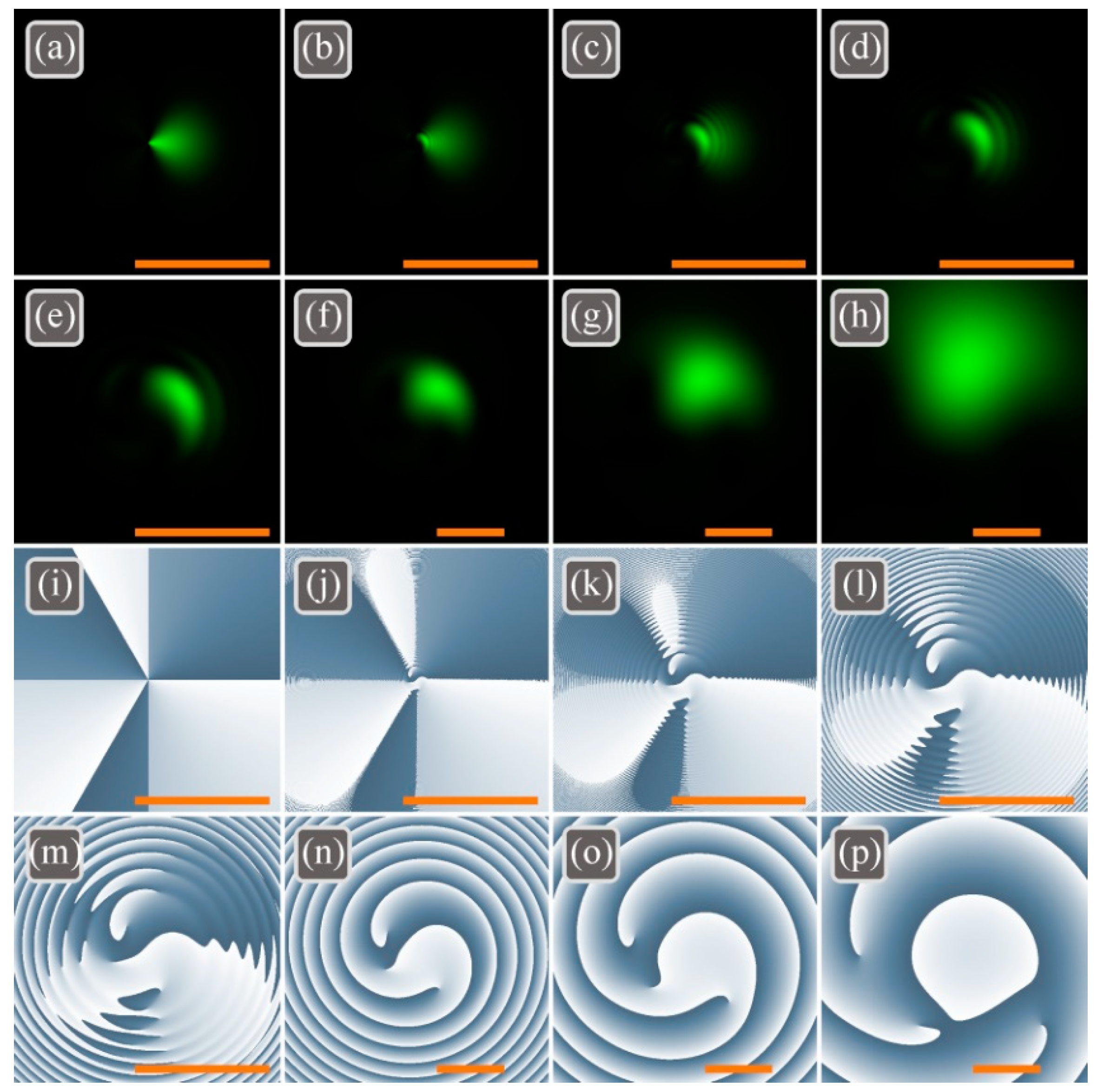
Figure 1 depicts the intensity and the phase distributions of the light field (33) with
n = 3,
k = 0,
m = 1,
a = 1,
w0 = 500 μm, wavelength λ = 532 nm,
z0 = 1476 mm in different transverse planes:
z = 0 (
Figure 1a,i),
z =
z0/200 (
Figure 1b,j),
z =
z0/50 (
Figure 1c,k),
z =
z0/20 (
Figure 1d,l),
z =
z0/10 (
Figure 1e,m),
z =
z0/2 (
Figure 1f,n),
z =
z0 (
Figure 1g,o),
z = 2
z0 (
Figure 1h,p).
Figure 1a confirms that the intensity distribution in the initial plane is shaped as a lobe (
m = 1) elongated along the positive direction of the horizontal axis. However, the divergence of OVs increases with their TC. Therefore, all the constituent vortices in the superposition (1) diverge differently, and the lobe splits into light bows during propagation, as it can be seen in
Figure 1b–d. Then, during further propagation, only one intensity spot remains in the picture (
Figure 1f–h) since the higher divergence of vortices with a large TC leads to their stronger attenuation.
The numerical computation of TC by M.V. Berry’s Equation (36) yields the following values: 1.49 (z = 0), 0.98 (z = z0/200), 2.29 (z = z0/50), 2.97 (z = z0/20), 2.97 (z = z0/10), 2.99 (z = z0/2), 3.00 (z = z0), 3.00 (z = 2z0). Thus, the half-integer TC of n/2 in the initial plane (TC = 1.5) becomes integer n (TC = 3) during propagation.
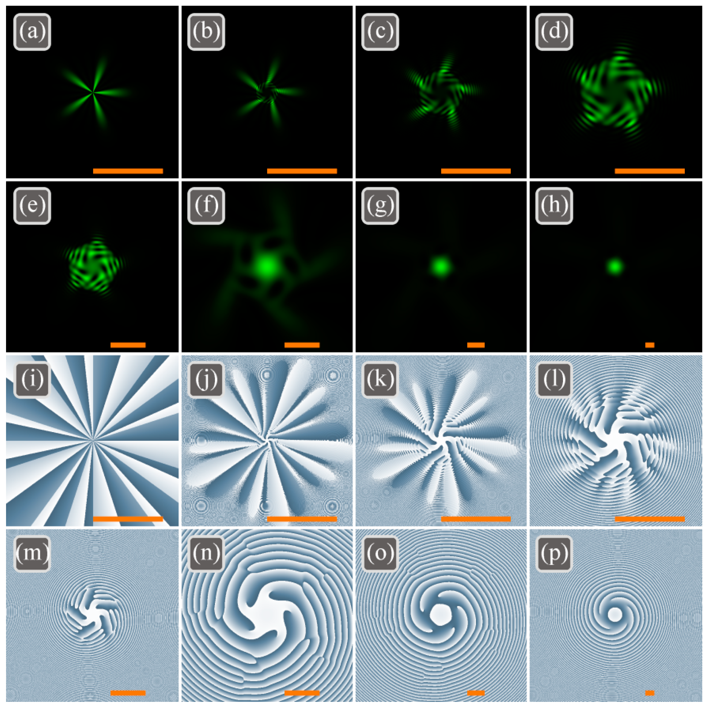
To demonstrate the influence of the TC increment
m in the progression,
Figure 2 depicts the intensity and the phase distributions of the light field (33) with
n = 3,
k = 0,
m = 5,
a = 1,
w0 = 500 μm in different transverse planes:
z = 0 (
Figure 2a,i),
z =
z0/200 (
Figure 2b,j),
z =
z0/50 (
Figure 2c,k),
z =
z0/20 (
Figure 2d,l),
z =
z0/10 (
Figure 2e,m),
z =
z0/2 (
Figure 2f,n),
z =
z0 (
Figure 2g,o),
z = 2
z0 (
Figure 2h,p).
The numerical computation of the TC by M.V. Berry’s formula (36) gives the following values: 7.48 (z = 0), −1.37 (z = z0/200), 12.84 (z = z0/50), 14.64 (z = z0/20), 14.64 (z = z0/10), 14.98 (z = z0/2), 14.94 (z = z0), 14.77 (z = 2z0). Thus, the half-integer TC of mn/2 (TC = 7.5) in the initial plane acquires the integer value mn (TC = 15) during propagation in space.
Further we study how the TC changes when several first terms are removed from the progression (33), i.e., when
k ≠ 0.
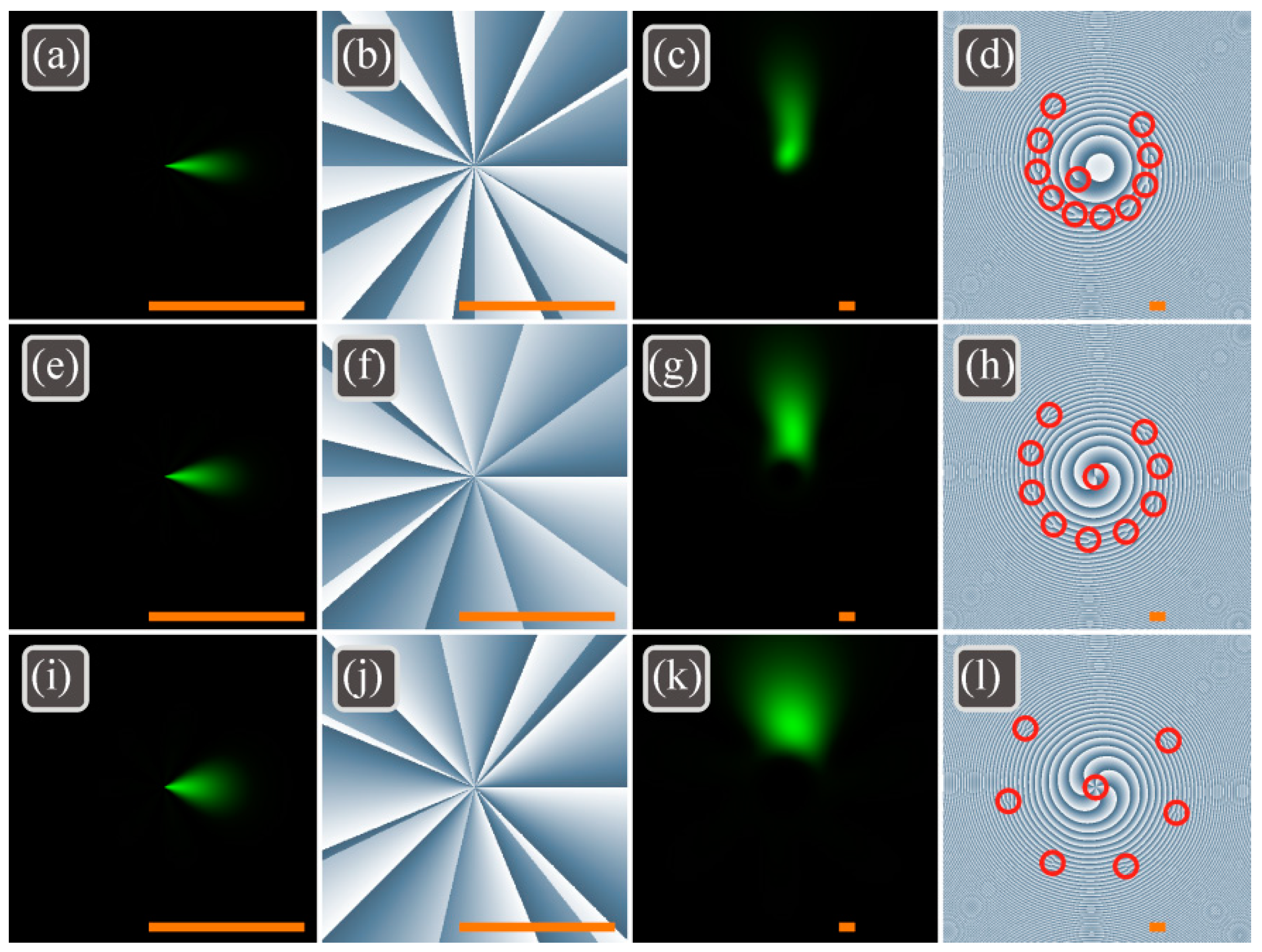
Figure 3 illustrates the intensity and the phase distributions of the light field (26) with
n = 11,
k = 0 (
Figure 3a–d),
k = 2 (
Figure 3e–h),
k = 5 (
Figure 3i–l),
m = 1,
a = 1,
w0 = 500 μm in the initial plane
z = 0 (
Figure 3a,b,e,f,i,j) and in the far field
z = 2
z0 (
Figure 3c,d,g,h,k,l).
The numerical computation of TC by M.V. Berry’s formula (36) yields the following values in the initial plane
z = 0: 5.49 (
k = 0), 6.49 (
k = 2), 7.99 (
k = 5). In the far field
z = 2
z0, the obtained values are 10.96 (for all
k, i.e.,
k = 0,
k = 2,
k = 5). Thus, the half-integer TC of (
n +
k)/2 in the initial plane becomes equal to the integer value
n (
TC = 11) during propagation. The OVs in
Figure 3 have a structure with an interesting property. An OV with the TC of
k = 0 (
Figure 3d),
k = 2 (
Figure 3h) and
k = 5 (
Figure 3l) is generated on the optical axis. This on-axis OV (
TC =
k = 0, 2, 5) is surrounded by vortices with the TC of +1 and the number of these vortices complements the total TC to
n = 11: 11 (
Figure 3d), 9 (
Figure 3h), and 6 (
Figure 3l). Thus, the total TC in all three cases in
Figure 3 is equal to 11.
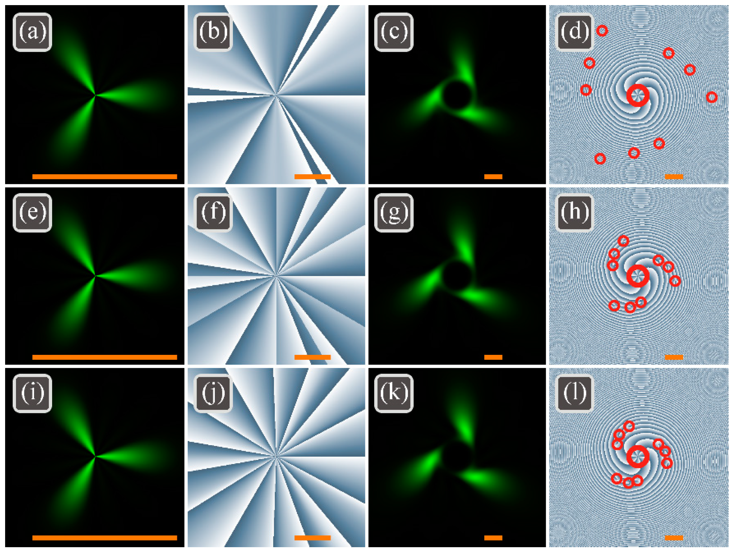
To demonstrate the influence of the continuous common ratio parameter
a,
Figure 4 depicts the intensity and the phase distributions of the light field (26) with
n = 5,
k = 2,
m = 3,
a = 0.8 (
Figure 4a–d),
a = 1.0 (
Figure 4e–h),
a = 1.2 (
Figure 4i–l),
w0 = 500 μm in the initial plane
z = 0 (
Figure 4a,b,e,f,i,j) and in the near field
z =
z0/2 (
Figure 4c,d,g,h,k,l).
As it can be seen in
Figure 4, all three beams have very similar intensity distributions both in the initial plane and after propagation in space. However, the phase distributions are different. The numerical computation of the TC by M.V. Berry’s Equation (17) yields the following values in the initial plane
z = 0: 6.00 (
a = 0.8), 10.49 (
a = 1.0), 14.99 (
a = 1.2). These values are consistent with Equation (38). However, the obtained values are 14.94 (for each
a, i.e.,
a = 0.8,
a = 1.0,
a = 1.2) even in the near field
z =
z0/2. Thus, the half-integer TC of (
n +
k)
m/2 in the initial plane becomes equal to the integer value
nm (
TC = 15) during propagation in space. Phase patterns in
Figure 4 reveal how the parameter
a affects the structure of the OVs. When
a < 1, the lowest-order vortex dominates (that is why the initial TC is
km = 6) and the peripheral vortices in
Figure 4d are far from the center. If, on the contrary,
a < 1, then the highest-order vortex prevails (that is why the initial TC is
nm = 15) and the peripheral vortices in
Figure 4l are close to the center, as if they were tending to merge into one 15th-order vortex at
. The total number of vortices in
Figure 4d,h,l is the same: 9 vortices of the 1st order and 1 vortex of the 6th order.
9. Experiment
In this section, we compare the intensity distributions of the beam (33) with
n = 3,
k = 0,
m = 5,
a = 1,
w0 = 500 μm (
Figure 2), which have been computed by the Fresnel transform and the generated experimentally by a spatial light modulator (SLM).
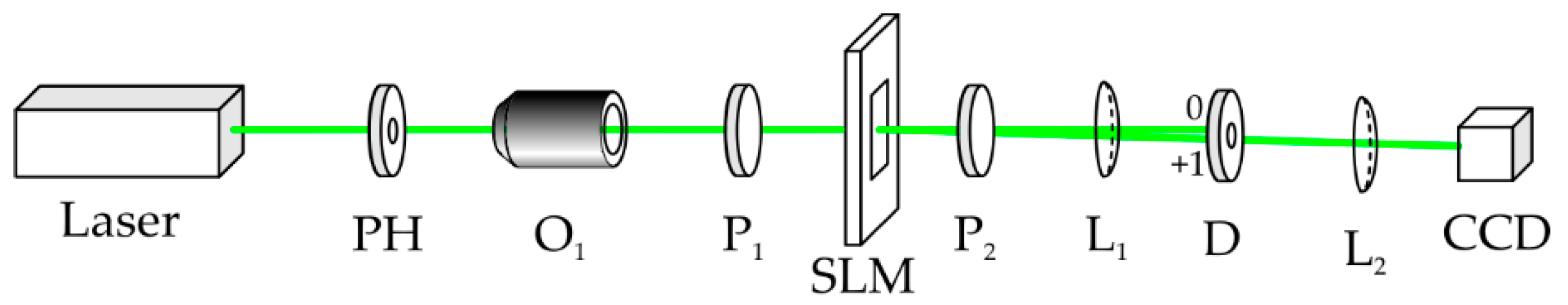
Figure 5 depicts an optical setup for the experiment. A linearly polarized Gaussian beam with the wavelength of 532 nm radiated by the laser and expanded by the micro-objective O
1 incidences normally onto the SLM. An OV whose amplitude is a geometric progression of simple vortices (33) is obtained after the SLM. Only the required diffraction order passes through a small diaphragm D and its intensity distribution is registered by a CCD-camera at a certain distance.
Since the SLM is phase-only, we applied to it only the phase of the light field (33) with
n = 3,
k = 0,
m = 5,
a = 1.
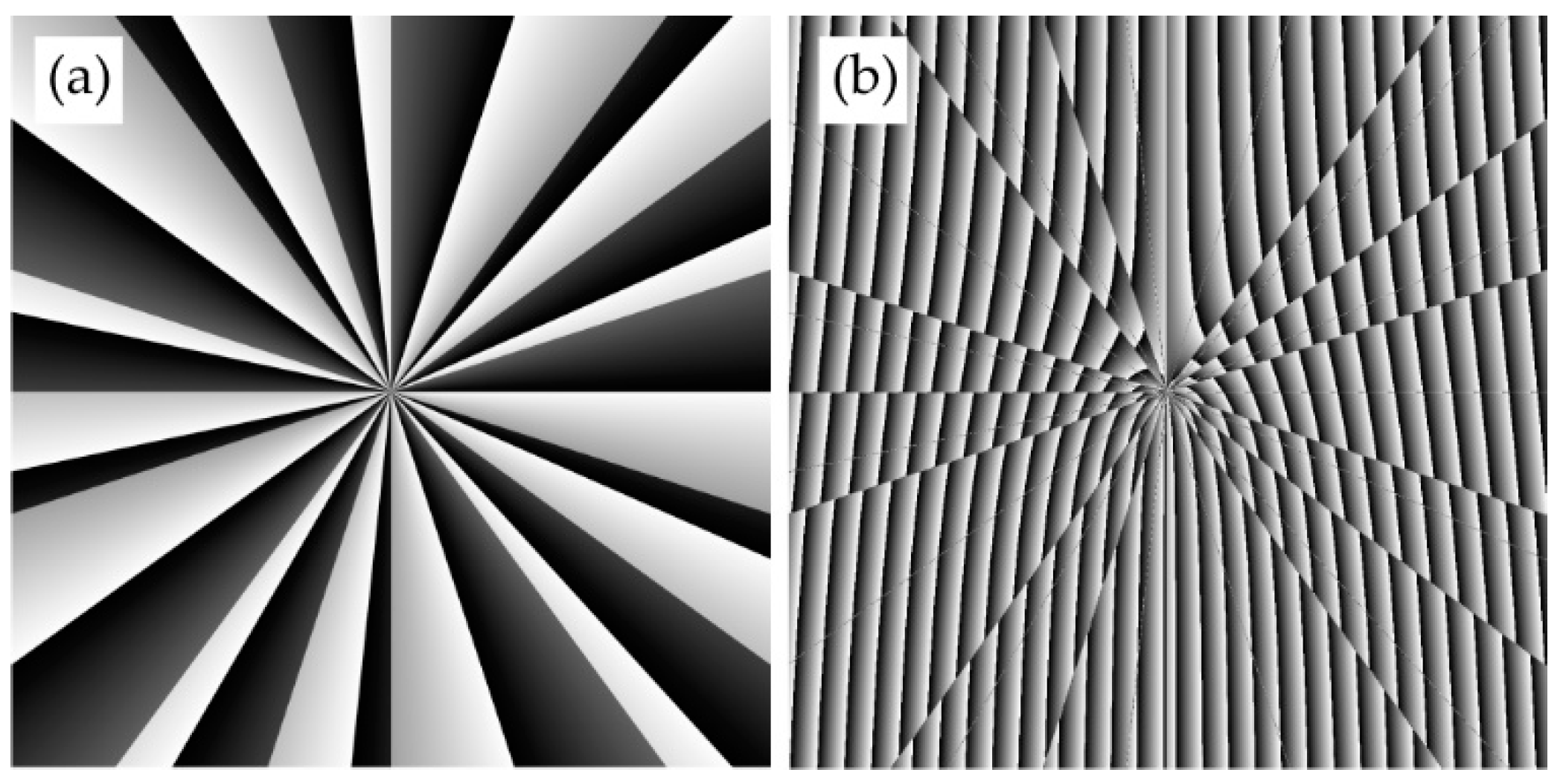
Figure 6a depicts only the phase of the beam (33). The black color in
Figure 6a means zero phase and the white color means 2π. The phase from
Figure 6a was applied to the SLM with a carrier spatial frequency (
Figure 6b) to generate the given beam in the first diffraction order.
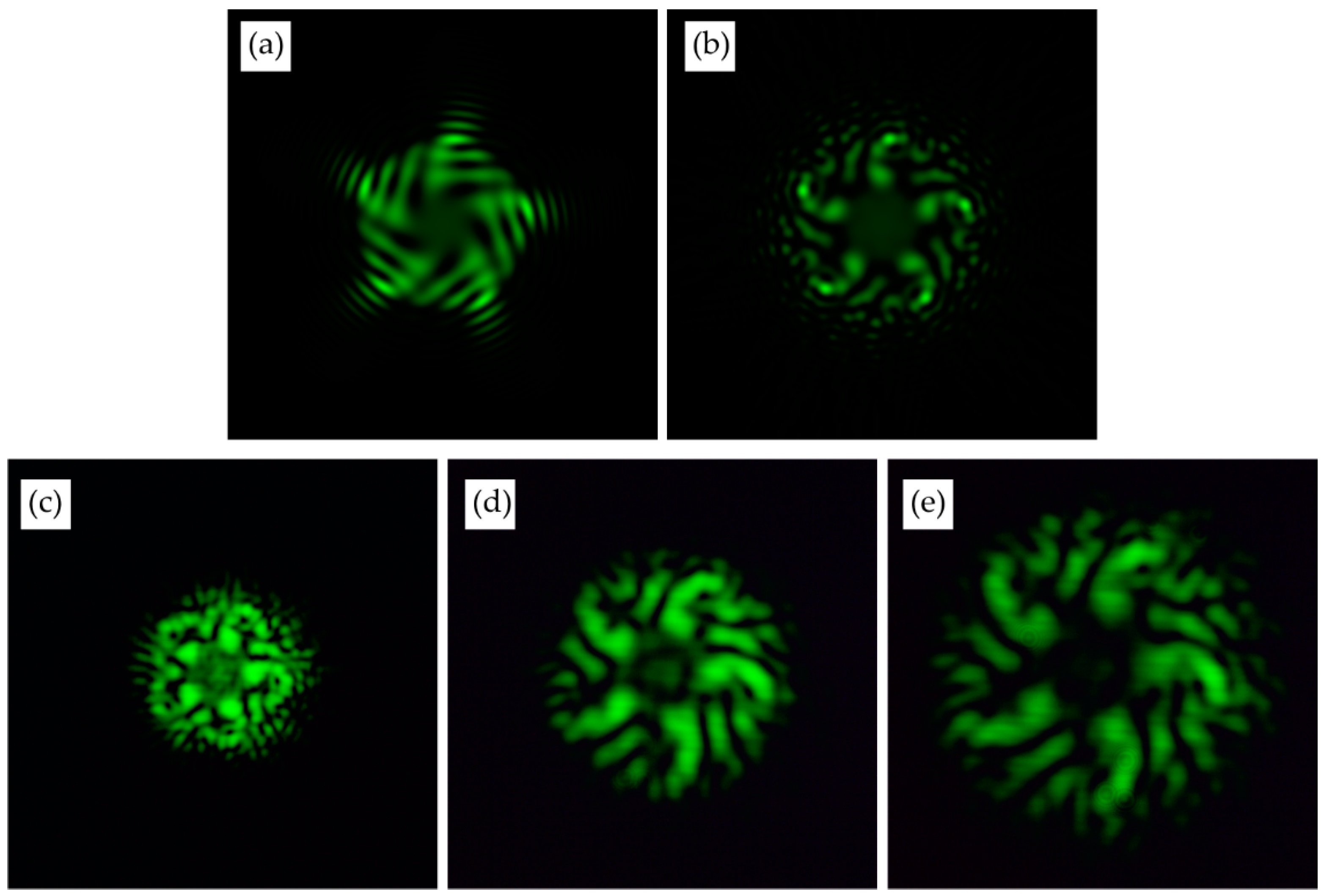
Figure 7a shows the intensity distribution of the beam (33) with
n = 3,
k = 0,
m = 5,
a = 1 (
w0 = 500 μm) computed by the Fresnel transform at a distance
z = 147 mm from the initial plane. This intensity (
Figure 7a) coincides with the intensity in
Figure 2e.
Figure 7b shows the computed intensity distribution that occurs after propagation of the pure-phase beam (33) with
n = 3,
k = 0,
m = 5,
a = 1, i.e., with ignoring the initial amplitude distribution (the amplitude is a Gaussian function with the waist radius of
w0 = 500 μm). Comparison of patterns in
Figure 7a,b indicates that despite the intensity distributions are different the 5th-order symmetry is retained.
Figure 7c illustrates the experimental intensity distribution obtained by the optical setup from
Figure 5 and applying the phase from
Figure 6b to the SLM. Comparison of simulation and experimental results shows their qualitative agreement.
10. Conclusions
In this study, we derived the topological charge (TC) of a four-parametric family of vortex beams whose complex amplitude is described by a geometric progression of the Gaussian optical vortices (OVs). This progression can be either growing, when the amplitudes of the constituent vortices increase, or decaying, or stationary. The first and the last terms in this progression are equal to
and
, respectively, i.e., the common ratio is
. The studied vortex beams family is described by three integer parameters (
k, n, m) and by one real parameter
a. If
a < 1, the progression is decaying and the TC of the whole superposition is equal to the TC of its first term (
TC =
km, k <
n), since this term describes an OV of the maximum power in the superposition. If
a > 1, the progression is growing and its TC is equal to the TC of the last term (
TC =
nm), since this term has the maximal power in the superposition. Finally, if
a = 1, the progression is stationary, its OAM-spectrum is symmetric, and the TC of the whole superposition is equal to the order of the average angular harmonic (
TC = (
k +
n)
m/2). In the latter case, the superposition can have a half-integer TC in the initial plane. However, the TC of the stationary progression of OVs becomes integer (
TC =
nm) and does not change during propagation in free space. Earlier, it was shown [
38] that if a spiral phase plate with the transmittance exp(
inφ) is fabricated for a specific wavelength λ
0 and illuminated by a laser light of another wavelength λ, then the TC
n becomes fractional
n(λ
0/λ) and, according to [
35], upon free-space propagation the number of vortices should double and the TC should become integer and equal to 2
n (if λ < λ
0). However, this conclusion is approximate, since the TC of an initial fractional OV becomes undefined during propagation in free space [
39], whereas for the geometric progression of OVs, the half-integer initial TC (
TC =
n/2) changes to the definite integer value, which is twice higher (
TC =
n).
The studied geometric progression of OVs with a wide OAM-spectrum occur when simple OVs are distorted by obstacles, for instance, by diaphragms, as in [
2].
The GPOVs have an unconventional shape for the OVs: instead of the ring-shape intensity, the intensity has a maximum (
Figure 2h), and OVs reside outside this intensity maximum (
Figure 2p). This property of the GPOVs can be used for trapping microscopic particles [
16]. A dielectric spherical microparticle of a certain size can be trapped by such a beam into the maximal-intensity area and rotate around its center of mass, due to the OVs of the same sign surrounding the focal spot. These vortices (
Figure 2p) will transfer to the particle some portion of their OAM which is equal to the TC of the entire beam.

 ,
, 


