Mapping the Stability and Dynamics of Optically Injected Dual State Quantum Dot Lasers

Abstract
:1. Introduction
2. Results
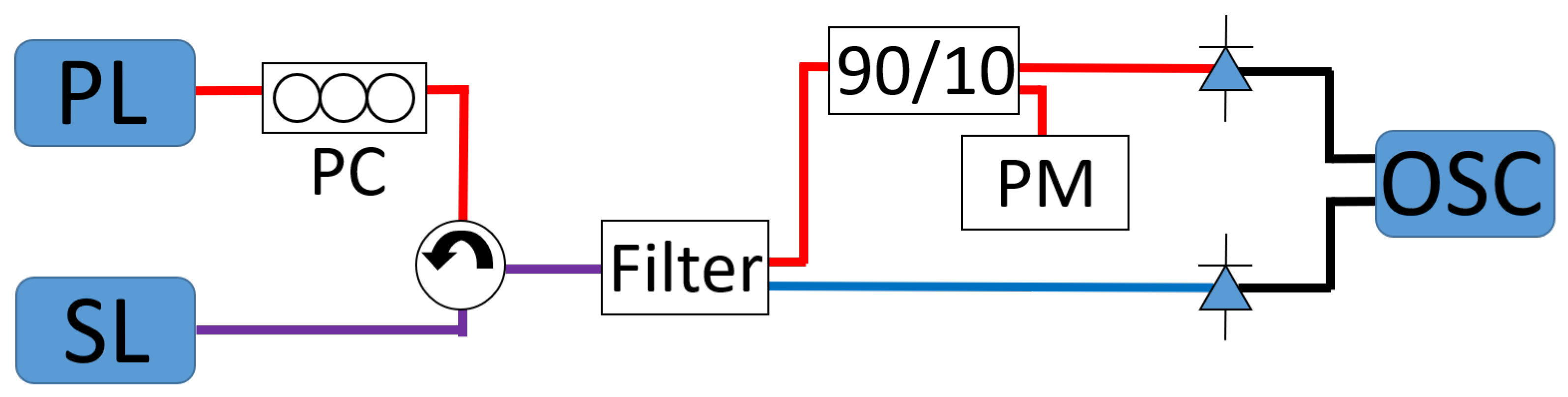
2.1. Experiment
2.1.1. Stability Maps
2.1.2. Hysteresis and Bistabilty
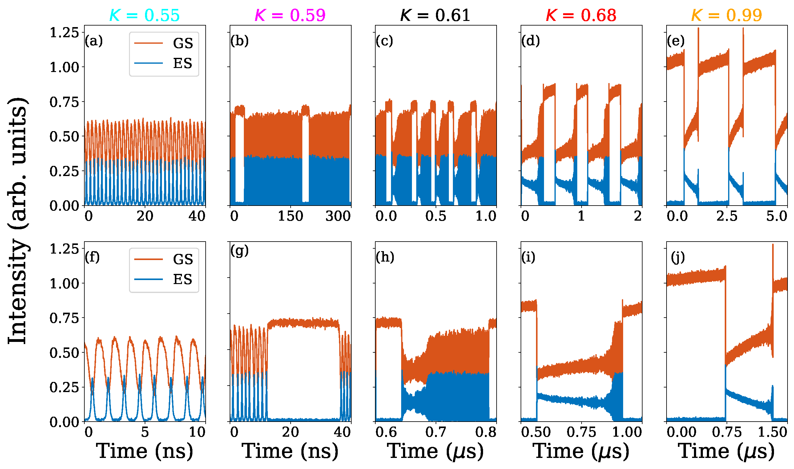
2.1.3. Slow Oscillations
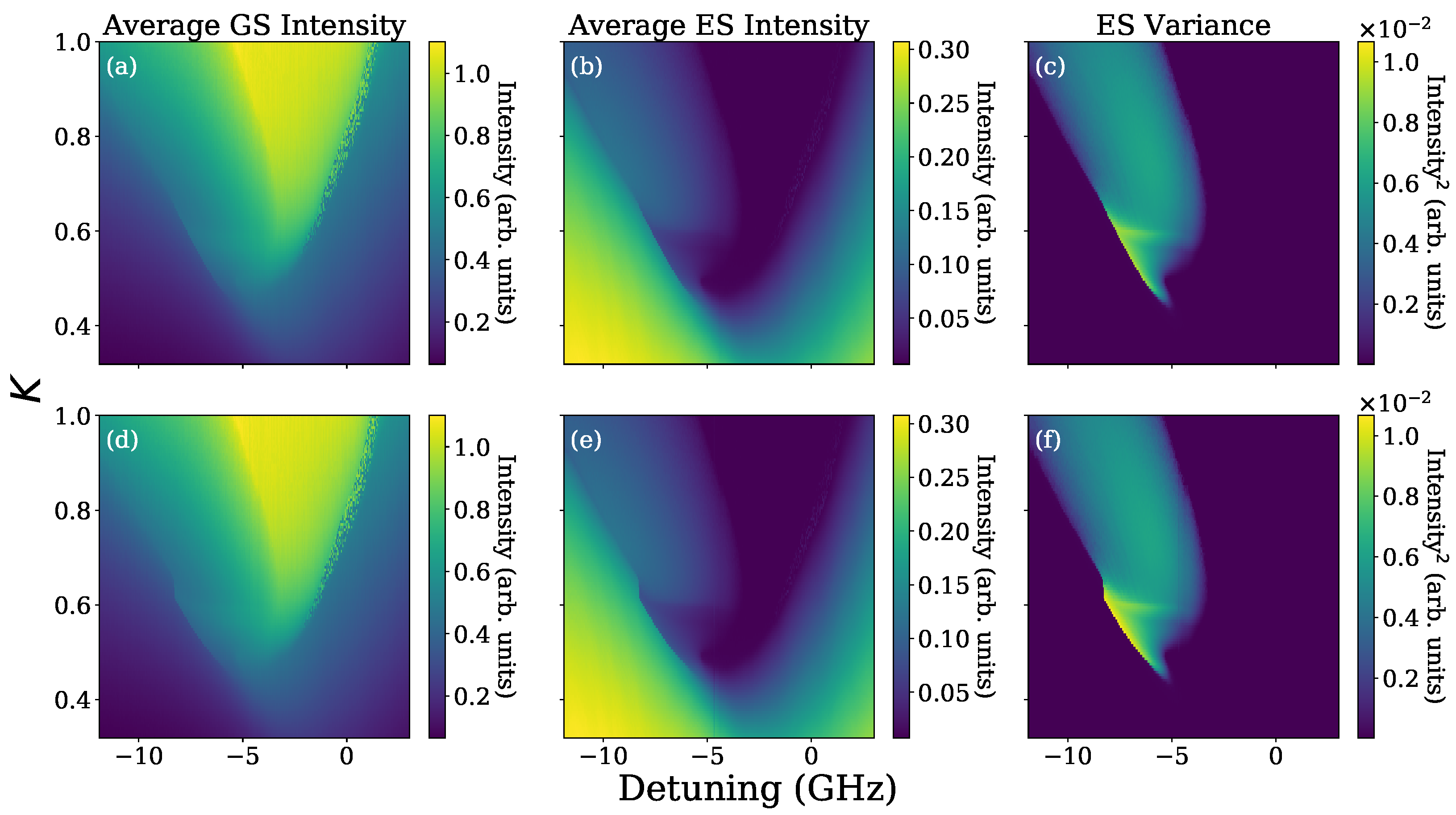
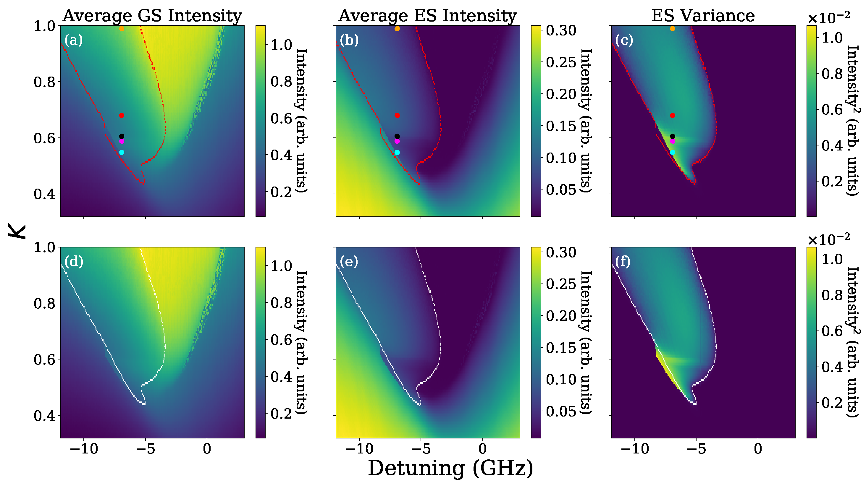
2.2. Theory
2.2.1. No Optothermal Effects
2.2.2. First Optothermal Effect
2.2.3. Second Optothermal Effect
2.2.4. Absence of Chaos
3. Discussion
Supplementary Materials
Author Contributions
Funding
Conflicts of Interest
References
- Wieczorek, S.; Krauskopf, B.; Simpson, T.; Lenstra, D. The dynamical complexity of optically injected semiconductor lasers. Phys. Rep. 2005, 416, 1. [Google Scholar] [CrossRef]
- O’Shea, D.; Osborne, S.; Blackbeard, N.; Goulding, D.; Kelleher, B.; Amann, A. Experimental classification of dynamical regimes in optically injected lasers. Opt. Express 2014, 22, 21701. [Google Scholar] [CrossRef] [PubMed]
- Kelleher, B.; Goulding, D.; Hegarty, S.; Huyet, G.; Viktorov, E.; Erneux, T. Optically injected single-mode quantum dot lasers. In Quantum Dot Devices; Springer: New York, NY, USA, 2012; pp. 1–22. [Google Scholar]
- Chan, S.-C. Analysis of an Optically Injected Semiconductor Laser for Microwave Generation. IEEE J. Quantum Electron. 2010, 46, 421. [Google Scholar] [CrossRef] [Green Version]
- Hurtado, A.; Mee, J.; Nami, M.; Henning, I.D.; Adams, M.J.; Lester, L.F. Tunable microwave signal generator with an optically-injected 1310 nm QD-DFB laser. Opt. Express 2013, 21, 10772. [Google Scholar] [CrossRef]
- Li, X.-Z.; Chan, S.-C. Random bit generation using an optically injected semiconductor laser in chaos with oversampling. Opt. Lett. 2012, 37, 2163. [Google Scholar] [CrossRef] [Green Version]
- Prucnal, P.R.; Shastri, B.J.; de Lima, T.F.; Nahmias, M.A.; Tait, A.N. Recent progress in semiconductor excitable lasers for photonic spike processing. Adv. Opt. Photonics 2016, 8, 228. [Google Scholar] [CrossRef]
- Gavrielides, A.; Kovanis, V.; Erneux, T. Analytical stability boundaries for a semiconductor laser subject to optical injection. Opt. Commun. 1997, 136, 253. [Google Scholar] [CrossRef]
- Erneux, T.; Viktorov, E.; Kelleher, B.; Goulding, D.; Hegarty, S.; Huyet, G. Optically injected quantum-dot lasers. Opt. Lett. 2010, 35, 937. [Google Scholar] [CrossRef] [Green Version]
- Mayol, C.; Toral, R.; Mirasso, C.R.; Natiello, M.A. Class-a lasers with injected signal: Bifurcation set and Lyapunov–potential function. Phys. Rev. A 2002, 66, 013808. [Google Scholar] [CrossRef] [Green Version]
- Chlouverakis, K.E.; Adams, M.J. Stability maps of injection-locked laser diodes using the largest Lyapunov exponent. Opt. Commun. 2003, 216, 405. [Google Scholar] [CrossRef]
- Bonatto, C.; Garreau, J.C.; Gallas, J.A.C. Self-similarities in the frequency-amplitude space of a loss-modulated CO2 laser. Phys. Rev. Lett. 2005, 95, 143905. [Google Scholar] [CrossRef] [PubMed] [Green Version]
- Kelleher, B.; Bonatto, C.; Huyet, G.; Hegarty, S. Excitability in optically injected semiconductor lasers: Contrasting quantum-well-and quantum-dot-based devices. Phys. Rev. E 2011, 83, 026207. [Google Scholar] [CrossRef] [PubMed]
- Dillane, M.; Tykalewicz, B.; Goulding, D.; Garbin, B.; Barland, S.; Kelleher, B. Square wave excitability in quantum dot lasers under optical injection. Opt. Lett. 2019, 44, 347. [Google Scholar] [CrossRef] [Green Version]
- Kelleher, B.; Tykalewicz, B.; Goulding, D.; Fedorov, N.; Dubinkin, I.; Erneux, T.; Viktorov, E.A. Two-color bursting oscillations. Sci. Rep. 2017, 7, 8414. [Google Scholar] [CrossRef] [Green Version]
- Dillane, M.; Robertson, J.; Peters, M.; Hurtado, A.; Kelleher, B. Neuromorphic dynamics with optically injected quantum dot lasers. Eur. Phys. J. B 2019, 92, 1. [Google Scholar] [CrossRef]
- Lingnau, B.; Lüdge, K.; Chow, W.W.; Schöll, E. Failure of the α factor in describing dynamical instabilities and chaos in quantum-dot lasers. Phys. Rev. E 2012, 86, 065201. [Google Scholar] [CrossRef] [PubMed] [Green Version]
- Lingnau, B.; Dillane, M.; O’Callaghan, J.; Corbett, B.; Kelleher, B. Multimode dynamics and modeling of free-running and optically injected fabry-pérot quantum-dot lasers. Phys. Rev. A 2019, 100, 063837. [Google Scholar] [CrossRef]
- Markus, A.; Chen, J.X.; Paranthoën, C.; Fiore, A.; Platz, C.; Gauthier-Lafaye, O. Simultaneous two-state lasing in quantum-dot lasers. Appl. Phys. Lett. 2003, 82, 1818–1820. [Google Scholar] [CrossRef]
- Bimberg, D.; Kirstaedter, N.; Ledentsov, N.; Alferov, Z.I.; Kop’Ev, P.; Ustinov, V. Ingaas-gaas quantum-dot lasers. IEEE J. Sel. Top. Quantum Electron. 1997, 3, 196. [Google Scholar] [CrossRef]
- Tykalewicz, B.; Goulding, D.; Hegarty, S.P.; Huyet, G.; Dubinkin, I.; Fedorov, N.; Erneux, T.; Viktorov, E.A.; Kelleher, B. Optically induced hysteresis in a two-state quantum dot laser. Opt. Lett. 2016, 41, 1034. [Google Scholar] [CrossRef]
- Tykalewicz, B.; Goulding, D.; Hegarty, S.P.; Huyet, G.; Byrne, D.; Phelan, R.; Kelleher, B. All-optical switching with a dual-state, single-section quantum dot laser via optical injection. Opt. Lett. 2014, 39, 4607. [Google Scholar] [CrossRef]
- Viktorov, E.A.; Dubinkin, I.; Fedorov, N.; Erneux, T.; Tykalewicz, B.; Hegarty, S.P.; Huyet, G.; Goulding, D.; Kelleher, B. Injection-induced, tunable all-optical gating in a two-state quantum dot laser. Opt. Lett. 2016, 41, 3555. [Google Scholar] [CrossRef] [Green Version]
- Dillane, M.; Dubinkin, I.; Fedorov, N.; Erneux, T.; Goulding, D.; Kelleher, B.; Viktorov, E.A. Excitable interplay between lasing quantum dot states. Phys. Rev. E 2019, 100, 012202. [Google Scholar] [CrossRef] [PubMed]
- Simpson, T.B.; Liu, J.M.; Huang, K.F.; Tai, K. Nonlinear dynamics induced by external optical injection in semiconductor lasers. Quantum Semiclass. Opt. 1997, 9, 765. [Google Scholar] [CrossRef]
- Desroches, M.; Guckenheimer, J.; Krauskopf, B.; Kuehn, C.; Osinga, H.M.; Wechselberger, M. Mixed-mode oscillations with multiple time scales. SIAM Rev. 2012, 54, 211. [Google Scholar] [CrossRef]
- Desroches, M.; Kaper, T.J.; Krupa, M. Mixed-mode bursting oscillations: Dynamics created by a slow passage through spike-adding canard explosion in a square-wave burster. Chaos 2013, 23, 046106. [Google Scholar] [CrossRef] [PubMed] [Green Version]
- Rzhanov, Y.A.; Richardson, H.; Hagberg, A.A.; Moloney, J.V. Spatiotemporal oscillations in a semiconductor étalon. Phys. Rev. A 1993, 47, 1480. [Google Scholar] [CrossRef]
- Abraham, E. Modelling of regenerative pulsations in an InSb etalon. Opt. Commun. 1987, 61, 282. [Google Scholar] [CrossRef]
- Bera, D.; Qian, L.; Tseng, T.-K.; Holloway, P.H. Quantum dots and their multimodal applications: A review. Materials 2010, 3, 2260. [Google Scholar] [CrossRef] [Green Version]
- Ziegler, M.; Tomm, J.W.; Elsaesser, T.; Erbert, G.; Bugge, F.; Nakwaski, W.; Sarzała, R.P. Visualization of heat flows in high-power diode lasers by lock-in thermography. Appl. Phys. Lett. 2008, 92, 103513. [Google Scholar] [CrossRef]
- Meinecke, S.; Lingnau, B.; Röhm, A.; Lüdge, K. Stability of Optically Injected Two-State Quantum-Dot Lasers. Ann. Phys. 2017, 529, 1600279. [Google Scholar] [CrossRef]
- Meinecke, S.; Lingnau, B.; Lüdge, K. Increasing stability by two-state lasing in quantum-dot lasers with optical injection. In Physics and Simulation of Optoelectronic Devices XXV. San Francisco, California, United States; Witzigmann, B., Osiński, M., Arakawa, Y., Eds.; International Society for Optics and Photonics (SPIE): Bellingham, WA, USA, 2017; Volume 10098, pp. 67–77. [Google Scholar]
- Pausch, J.; Otto, C.; Tylaite, E.; Majer, N.; Schöll, E.; Lüdge, K. Optically injected quantum dot lasers: Impact of nonlinear carrier lifetimes on frequency-locking dynamics. New J. Phys. 2012, 14, 053018. [Google Scholar] [CrossRef]
- O’Brien, D.; Hegarty, S.; Huyet, G.; McInerney, J.; Kettler, T.; Laemmlin, M.; Bimberg, D.; Ustinov, V.; Zhukov, A.; Mikhrin, S.; et al. Feedback sensitivity of 1.3/spl mu/m inas/gaas quantum dot lasers. Electron. Lett. 2003, 39, 1819. [Google Scholar] [CrossRef]
- O’Brien, D.; Hegarty, S.; Huyet, G.; Uskov, A. Sensitivity of quantum-dot semiconductor lasers to optical feedback. Opt. Lett. 2004, 29, 1072. [Google Scholar] [CrossRef] [PubMed]
- Duan, J.; Huang, H.; Dong, B.; Norman, J.C.; Zhang, Z.; Bowers, J.E.; Grillot, F. Dynamic and nonlinear properties of epitaxial quantum dot lasers on silicon for isolator-free integration. Photonics Res. 2019, 7, 1222. [Google Scholar] [CrossRef]
- Kelleher, B.; Dillane, M.; Viktorov, E.A. Optical information processing using dual state quantum dot lasers: Complexity through simplicity. Lightw. Sci. Appl. 2021, 10, 238. [Google Scholar] [CrossRef] [PubMed]


| Symbol | Value | Meaning |
|---|---|---|
| J | Normalised pump current | |
| 2 | Phase-amplitude coupling from the GS | |
| Phase-amplitude coupling from the ES | ||
| g | Optical gain coefficient | |
| Optical loss coefficient | ||
| Spontaneous emission factor | ||
| Charge-carrier recombination time | ||
| QD capture rate | ||
| QD relaxation rate | ||
| Confinement energy of the ES | ||
| Energy separation between GS and ES | ||
| Normalised 2D density of states | ||
| T | Temperature | |
| Characteristic time scale of non-radiative thermal effects | ||
| Characteristic time scale of reabsorption thermal effects |
Publisher’s Note: MDPI stays neutral with regard to jurisdictional claims in published maps and institutional affiliations. |
© 2022 by the authors. Licensee MDPI, Basel, Switzerland. This article is an open access article distributed under the terms and conditions of the Creative Commons Attribution (CC BY) license (https://creativecommons.org/licenses/by/4.0/).
Share and Cite
Dillane, M.; Lingnau, B.; Viktorov, E.A.; Kelleher, B. Mapping the Stability and Dynamics of Optically Injected Dual State Quantum Dot Lasers. Photonics 2022, 9, 101. https://doi.org/10.3390/photonics9020101
Dillane M, Lingnau B, Viktorov EA, Kelleher B. Mapping the Stability and Dynamics of Optically Injected Dual State Quantum Dot Lasers. Photonics. 2022; 9(2):101. https://doi.org/10.3390/photonics9020101
Chicago/Turabian StyleDillane, Michael, Benjamin Lingnau, Evgeny A. Viktorov, and Bryan Kelleher. 2022. "Mapping the Stability and Dynamics of Optically Injected Dual State Quantum Dot Lasers" Photonics 9, no. 2: 101. https://doi.org/10.3390/photonics9020101