Article

Numerical and Monte Carlo Simulation for Polychromatic L-Shell X-ray Fluorescence Computed Tomography Based on Pinhole Collimator with Sheet-Beam Geometry

1
Chongqing Key Laboratory of Optical Fiber Sensor and Photoelectric Detection, Chongqing University of Technology, Chongqing 400054, China
2
The Central Hospital Affiliated to Chongqing University of Technology, Chongqing 400054, China
*
Author to whom correspondence should be addressed.
Photonics 2022, 9(12), 928; https://doi.org/10.3390/photonics9120928
Submission received: 17 October 2022 / Revised: 26 November 2022 / Accepted: 29 November 2022 / Published: 2 December 2022
(This article belongs to the Special Issue Computational Optical Imaging and Its Applications)

Abstract

:
X-ray fluorescence computed tomography (XFCT) has attracted wide attention due to its ability to simultaneously and nondestructively obtain structural and elemental distribution information within samples. In this paper, we presented an image system based on the pinhole collimator for the polychromatic L-shell XFCT to reduce time consumption and improve the detection limit. First, the imaging system model was expressed by formulas and discretized. Then, two phantoms (A and B) were scanned by numerical simulation and Monte Carlo simulation. Both phantoms with the same diameter (10 mm) and height (10 mm) were cylinders filled with PMMA, and embedded with GNP-loaded cylinders. The phantom A was inserted by six 1.5 mm-diameter cylinders with different Au concentrations ranging from 0.2% to 1.2%. The phantom B was inserted by eight cylinders with the same Au concentration (1%), but a radius ranging from 0.1 mm to 0.8 mm. Finally, the reconstruction of the XFCT images was performed using the method with and without absorption correction, respectively. The feasibility of XFCT system presented in this paper was demonstrated by the numerical simulation and the Monte Carlo simulation. The results show that absorption attenuation can be corrected by the presented method, and the contrast to noise ratio (CNR) is proportional to Au concentration but almost remains unchanged with the radius of GNP-loaded cylinders, which may provide the necessary justification for further optimization of the imaging system.

1. Introduction

X-ray fluorescence CT has caused widespread concern due to its ability to detect and quantify the elemental composition and distributions within samples in a nondestructive and noninvasive method [1,2]. Usually, fluorescence X-rays will be emitted from samples and measured with a detector when high-Z atomic numbers elements interact with incident X-rays. Projections acquired by rotating the X-ray tube or phantom are used to reconstruct the distribution and content of the elements [3].
Due to its high atomic number and low toxicity, gold nanoparticles (GNPs) are an ideal contrast agent and nanoprobes in biological imaging and medical diagnostics [4,5]. At present, K-shell XFCT with GNPs has been developed due to its greater depth in biological tissue [6]. However, the detection limits of XFCT imaging systems presented by several groups range from 5 to 20 mg Au/mL [7,8], and it cannot meet the requirement of in vivo imaging for small animals, where detection limits must be from 1 to 60 μg/mL [6]. In order to improve the detection performance of GNPs, L-shell fluorescent X-rays are taken into consideration. Although L-shell fluorescent X-rays have a three times lower yield than K-shell X-rays, they have an approximately 20 times higher cross-section than K-shell X-rays. Therefore, the detection limits of L-shell XFCT can be theoretically improved by seven times compared with K-shell XFCT [9,10].
There were some simulations and experimental research on L-shell XFCT [10,11,12,13]. Liu Long et al. provided the attenuation correction of L-shell XFCT and proved the feasibility by the Geant4 simulation. Magdalena, et al. simulated L-shell XFCT imaging of Cisplatin, and then experimental validation was performed with gold chloride. Their investigations found that conventional imaging geometries have the disadvantage of consuming time. Pinhole collimator, slit collimator and multi-pinhole collimator have been proposed by some researchers to solve the problem [14,15]. However, at present, there are few examples of literature that apply these imaging methods to L-shell XFCT. In references [15,16], sheet-beam was used to simplify the formulation of the measurement process.
Therefore, an imaging system model based on the pinhole collimator with sheet-beam geometry was presented for polychromatic L-shell X-ray fluorescence computed tomography in this work. Then, the model was expressed by formulas and discretized. Two phantoms (A and B) inserted with GNP-loaded cylinders were scanned by numerical simulation and Monte Carlo simulation. The reconstruction of the XFCT images were performed using the method with and without absorption correction, respectively. At last, the contrast-to-noise ratio (CNR) was used to evaluate the quality of reconstruction images, and the relationship between the CNR and Au concentration and radius of GNPs-loaded cylinders was discussed.

2. Materials and Methods
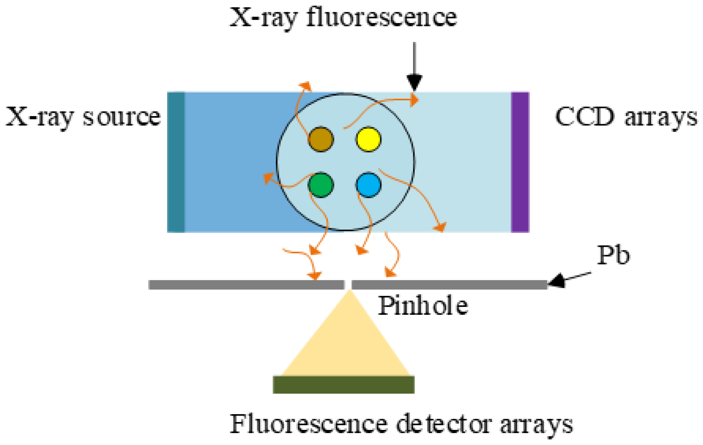
2.1. Imaging System

Figure 1 shows the imaging principle of the system presented in this work, which consists of polychromatic X-ray source, pinhole collimator, fluorescent array detectors and CCD [17,18].
The X-rays are shaped into parallel sheet beams by a lead collimator, incident on the phantom and cover the entire imaging section. Then, fluorescent X-rays are emitted isotropically due to the interaction of X-rays with high Z elements. The X-rays that pass through the pinhole are recorded by linear array detectors with energy resolution. All recorded data are stored on the computer for image reconstruction.

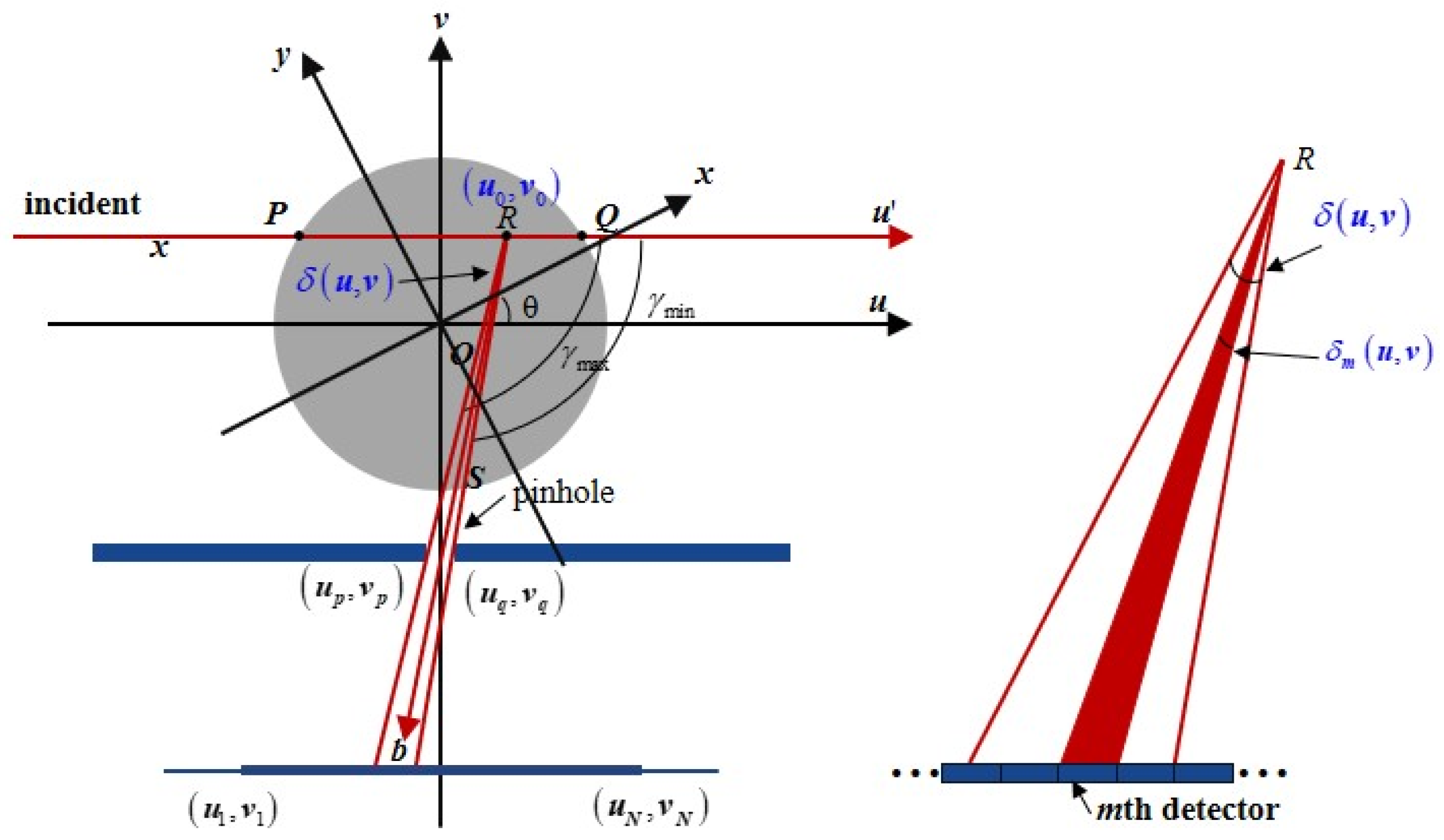
2.2. Geometry Model of XFCTB Based on Pinhole

To describe the imaging model by formula, two coordinate systems are established, as shown in Figure 2. We assumed that the X-ray source, pinhole collimator and detector were stationary and fixed to the uv-coordinate, while the phantom was rotary and fixed to the xy-coordinate. The uv-coordinate can be represented at any time by the xy-coordinate rotating angle θ counterclockwise. The relationship between the two coordinate systems can be expressed:
u v = cos θ sin θ sin θ cos θ x y
As shown in Figure 2, the incident sheet-beam can be viewed as independent X-rays. Considering one of them, we assumed that the incident X-ray intersected the phantom at the line segment PQ, and point R is on the line segment that emits fluorescent photons. Then, the photons passed the pinhole to detector m. The process can be described as follows [19]:
Step1: When the incident X-ray passes from P to R, its intensity will be attenuated by the phantom. The flux at point R can be expressed as:
I R u , v = I 0 exp u μ I u , v d u
where I 0 represents the flux of incident X-rays, and μ I u , v represents the linear attenuation coefficient of the element at incident intensity.
Step2: The emitted X-rays at point R, which pass through pinhole, can be given by
μ p h Δ u ω I 0 δ u , v exp u μ I u , v d u ρ u , v
where μ p h is the photoelectric linear coefficient of the element, ω is the field of fluorescent X-ray, and ρ u , v is the element weight concentration. Δ u and δ u , v are the differential of u and solid angle at which the point, R, is viewed by the pinhole, respectively [20].
Step3: We number the fluorescent array detector with m ranging from 1 to M. Since the X-rays passing through pinhole may cover several fluorescent detectors, the angle δ should be divided into several parts according to the covered detectors. Considering the covered detector with number m, a single X-ray emitted from the point, R, reaching the mth detector, is attenuated along segment RS. Let μ F ( u , v ) be the linear attenuation coefficient of fluorescent X-ray. The attenuation of X-ray fluorescence can be expressed as
exp 0 μ F u b cos γ , v + b sin γ d b
The total attenuation of X-ray fluorescence emitted from point R is given by
γ min γ max exp 0 μ F u b cos γ , v + b sin γ d b d γ
The total intensity of the fluorescent X-ray, emitted from the segment PQ, reaching the mth detector, can be given by the following formula:
I = μ p h ω I 0 + δ m u , v exp s μ I u , v d u ρ u , v    γ min γ max exp 0 μ F u + b cos γ , v b sin γ d b d γ d u
where δ m u , v is the angle at point, R, viewed by the mth detector. The intensity of total emitted X-ray fluorescence reaching the mth detector is obtained by integrating with respect to v from negative infinity to positive infinity, which can be given by the following formula:
I m θ = μ p h ω I 0 + + δ m u , v exp u μ I u , v d u ρ u , v     γ min γ max exp 0 μ F u + b cos γ , v b sin γ d b d γ d u d v     = D δ m u , v f θ , u , v g θ , u , v ρ u , v d u d v
Here, integral region, D, is the part of the image section, where the emitted fluorescent X-rays can reach the mth detector and
f θ , u , v = I 0 exp u μ I u , v d u
g θ , s , t = μ p h ω γ min γ max exp 0 μ F u + b cos γ , v b sin γ d b d γ
If the μ I u , v 0 and μ F u , v 0 , Equation (7) can be expressed approximately as follows:
I m θ μ p h ω I 0 δ m D ρ u , v d u d v

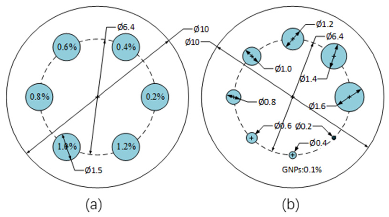
2.3. Numerical Simulation

To simulate the process of XFCT with the pinhole, we need to discretize Equation (7). The phantom is assumed to be two-dimensional. Here, the phantom is divided into N × N pixels in the xy-coordinate system. Let us number the pixels with j ranging from 1 to J. The parameters, μ j F , μ j I and ρ j , are corresponding to μ F u , v , μ I u , v and ρ u , v , where j means the number of pixels. We assumed that the phantom was irradiated by the X-ray source in different directions numbered with n (n = 1, 2, 3….D). For each direction, we number the incident X-ray with p ranging from 1 to P. The discretized process can be described in the following steps.
Step1: We define Sp as the set of pixels which are intersected with the pth incident X-ray [16]. Spj is the subset of Sp, denoting these pixels before reaching the jth pixel (Figure 3b). The length of segment line, which the pth X-ray intersects with the kth ( k S p j ) pixel, is defined as L p k I . The intensity of the incident X-ray before reaching the jth pixel is given by
f p j = I 0 exp k S p j μ k I L p k I
Step2: The emitted fluorescent X-rays from the jth pixel is proportional to the product of the intensity of the incident X-ray reaching the jth pixel and μ p h ω L p j I ρ j , where ρ j is the weight concentration of high Z element [16]. The total emitted fluorescent X-rays can be expressed as follows
μ p h ω f p j L p j I ρ j
Step3: Only those fluorescent X-rays passing through pinhole can be measured by array detectors. The fan-shaped fluorescent X-rays are considered several individual X-rays, which are also attenuated by the phantom. Let us number the individual fluorescent X-ray with l ranging from 1 to L. For each detector, the measured fluorescent X-ray is considered as one projection. Here, we will calculate the attenuation of the jth pixel to the detector numbered with m, which is covered by the fan-shaped fluorescent X-rays emitted from the jth pixel. Let us define the set of individual X-rays reaching the detector numbered with m as Km. Tzjlp is defined as the indexes consisting of the pixels intersected with the lth fluorescent X-ray. The attenuation of the jth pixel to the detector numbered with m can be expressed as follows
g m j = μ p h ω c a r d K m Δ δ 2 π l K m exp z T z j l p μ z F L z j l p F
where c a r d K m represents the number of the elements in set K m and Δ δ = δ / L . The relationship between i and m can be expressed as
i = n 1 M + m
Therefore, the attenuation of jth pixel to the ith projection is written by
g i j = g n 1 M + m = g m j = μ p h ω c a r d K m Δ δ 2 π l K m exp z T z j l p μ z F L z j l p F
Repeating Step1 to Step3, let h i j = f i j g i j L i j I and I i = j h i j ρ j , the matrix representation of Ii is given by
I = H ρ
where
H = h i j 1 i I ,   1 j J
I = I i 1 i I
ρ = ρ j 1 j J
The numerical simulation geometry in this study is shown in Figure 2. The proposed discretized method above was used to image phantoms (A and B) shown in Figure 4. Both phantoms are cylinders with the height and diameter of 10 mm. For phantom A, six small cylinders with GNPs are embedded and the diameter (1.5 mm) and height (10 mm) of these small cylinders are same, but the concentrations are different, ranging from 0.2% to 1.2%. Similarly, for phantom B, eight small cylinders with 1% GNPs are embedded, and their diameters are different, ranging from 0.2 mm to 1.6 mm. The pinhole radius is 100 μm. The distance from the pinhole to the center of the phantom and the distance from the pinhole to the array detector are both 4.5 cm. The incident X-ray flux rate is set to 1 × 10⁸ photons/cm2/s with 10 mm width of sheet beam. The phantoms are discretized into 128 × 128 pixels and scanned with a rotational step 3°.

2.4. Monte Carlo Simulation

Monte Carlo methods are usually implemented by software, such as Monte Carlo N Particle Transport Code (MCNP), Electron-Gama Shower four (EGS4) and GEometry ANd Tracking (GEANT). In this study, the imaging process was simulated by MCNP software.
We considered the imaging process of each projection angle as an independent simulation. In the whole projection process, the X-ray tube source was repeatedly simulated, which leads to excessive time consumption. A virtual source was used to replace the X-ray tube source simulation in order to reduce simulation time. Meanwhile, SpekCalc software was used to calculate its spectrum [21]. Allow a 62 keV electron beam to bombard a tungsten anode, and the anode’s emitted X-rays were filtered by 0.45 mm of aluminum. Figure 5 shows the spectrum of the sheet beam X-ray source. The 10 mm-width sheet beam was used to scan the phantoms. As the same as the numerical simulation, the positions of pinhole and fluorescent array detectors remained unchanged. The array detectors consist of 128 elements with energy resolution. All fluorescent X-rays and Compton scattering X-rays can be recorded by each element of the array detector from 6.5 keV to 62 keV with an interval of 0.5 keV. During each simulation, 1 × 10⁸ histories were used and the uncertainty of relevant photon energy (8–13 keV) was less than 5%. In order to obtain fluorescent photons, the L-shell fluorescence peaks were eliminated by cubic polynomial fitting. For each detector, the difference between the measured photon and the fitted photon was considered as its recorded fluorescent photons [8]. In addition, all the simulated fluorescent photons were used to reconstruct the sinogram.

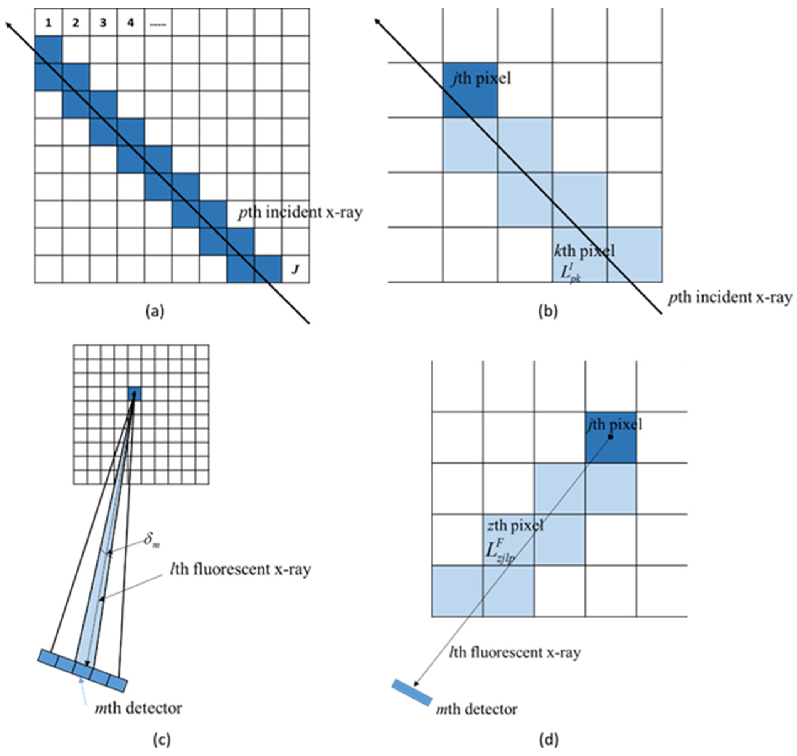
2.5. XFCT Image Reconstruction

In this work, the XFCT reconstructed images were obtained by the Maximum Likelihood Expectation Maximization (MLEM) algorithm. When absorption correction exists or does not exist, the XFCT images were reconstructed, respectively, to explore the impact of absorption from incident X-rays and fluorescent X-rays.
CNR was calculated to evaluate the XFCT images, which is the ratio of the difference between the mean value of each GNP-loaded region and background (PMMA) and the standard deviation of background. Therefore, CNR is expressed by the following formula [22].
C N R = Ψ ¯ Re g i o n Ψ ¯ B K V B K
where Ψ ¯ Re g i o n and Ψ ¯ B K are mean reconstructed values of GNP-loaded region and background, respectively. V B K is the standard deviation of background (PMMA). According to the Rose criterion, imaging sensitivity limit of the system proposed was determined using CNR of 4.

3. Results

3.1. Numerical Simulation

Figure 6 shows the sinograms of the two phantoms with GNP-loaded regions in the numerical simulations. The reconstructed XFCT images by the MLEM algorithm are shown in Figure 7. Figure 7a,c are the XFCT images of phantom A and B reconstructed by MLEM without attenuation correction, respectively, while Figure 7b,d are the XFCT images of phantom A and B reconstructed by MLEM with attenuation correction, respectively. The gray values in Figure 7a show an increase with the increase in Au weight concentration. Due to absorption attenuation, gray values of each GNP-loaded region are not uniform in uncorrected images. Even worse, some GNP-loaded regions are not disk-shaped in Figure 7c. Compared to uncorrected images, the corrected images have higher contrast and sharper edges than the uncorrected images in Figure 7b,d.
In Figure 7, we extract red lines through the center of each figure from left to right and plot the gray values of this line in Figure 8a,b, which shows that the corrected concentration is closer to the true value than the uncorrected one. The reconstructed Au weight concentration calculated from the mean value of each GNP-loaded region in phantom A and B is plotted in Figure 8c,d. Both figures indicate that the reconstructed Au concentrations are coincident with their true values after attenuation correction, and the corrected values have much smaller relative errors than the uncorrected ones, which means that self-absorption correction is a key step to reconstructing more accurate XFCT images.

3.2. Monte Carlo Simulation

The sinograms of the two phantoms (A and B) were acquired based on the previous description. Here, Figure 9a,b are the sinograms of phantom A and phantom B, respectively. Figure 10 shows XFCT images of the phantoms by MLEM. Obviously, the gray values still increase in Figure 10a,b while the Au weight concentration increases. Compared to uncorrected images, the corrected ones still have better contrast and sharper edges. In Figure 11d, when the radius of GNPs-loaded becomes smaller (<0.03 mm), the reconstructed concentration has larger relative errors, which may arise from the size of the pixel and the fluorescent detector element.
Processing the reconstructed images like in numerical simulation, the corrected concentrations (Figure 11b,d) are also closer to the true values than the uncorrected ones (Figure 11a,c). Due to the influence of absorption, the distribution of Au weight concentration in Figure 10a,c is not uniform. After absorption was corrected by the presented method, the uniformity of the concentration distribution (Figure 10b,d) still existed, but it was partially optimized.

3.3. CNR and Detection Limit

Figure 12 shows CNR for all the reconstructed images. CNR for reconstructed XFCT images in numerical simulation and Monte Carlo simulation as a function of Au weight concentration is presented in Figure 12a,c, respectively. Due to all the CNR values being greater than 4 in both figures, according to the Rose criterion, all GNPs-loaded regions can be detectable. In addition, the CNR of the corrected images is higher than the uncorrected images. Figure 12a,c show when the GNPs-loaded region has the same size as the value of CNR is linearly proportional to the Au weight concentration ( R 2 0.9966 ). CNR for reconstructed XFCT images in the numerical simulation and Monte Carlo simulation as a function of GNPs-loaded region size is also presented in Figure 12b,d, respectively. In both figures, CNR for the corrected images is also higher than the uncorrected ones. In numerical simulation (Figure 12b), CNR does not change significantly with a reduction in GNPs-loaded region radius in uncorrected and corrected images. However, in the Monte Carlo simulation, as the radius of the GNPs-loaded region gradually decreases from 0.8 mm to 0.1 mm, the CNR of the corrected image has a downward trend. Especially in the smallest region, the detectability will be significantly affected by the sharp decline of CNR.
The correction method presented in this study can improve the detection limit. According to the Rose criterion, the detection limits in the numerical simulation are 0.13% (uncorrected) and 0.05% (corrected), respectively. In the Monte Carlo simulation, the detection limits are 0.17% (uncorrected) and 0.14% (corrected), respectively.

4. Discussion and Conclusions

We presented an imaging model for polychromatic L-shell X-ray fluorescence computed tomography based on a pinhole collimator with sheet-beam geometry. Numerical and Monte Carlo methods were used to simulate the imaging process. The discretized model was presented to correct attenuation during image reconstruction.
Because synchrotron radiation is very expensive and bulky, the clinical application and research of XFCT is impossible for most researchers. During the Monte Carlo simulation, we replaced synchrotron radiation in similar systems presented previously by others with polychromatic X-rays, which helped to reduce cost and size of the apparatus and approach to the application [23,24,25]. Meanwhile, the X-ray source was collimated into a parallel sheet beam and radiated the whole imaging cross-section, and there was only rotation but no translation of the X-ray source, which may drastically reduce scanning time.
In Figure 12b,d, CNR did not almost change with the radius of the GNPs-loaded region, which is different from Lei Xing’s result, where CNR of the corrected images reconstructed by MLEM decreases with the reduction in GNPs-loaded region radius [9,12]. The smaller phantom size in our study may be one of the reasons for less attenuation of L-shell X-ray fluorescence, compared with the 2 cm and 4 cm phantoms in Lei Xing’s paper. In addition, for the same Au weight concentration, CNR may be mainly affected by photon scattering, which is suppressed by pinhole collimators in this study. Another reason should be the monochromatic source and whole ring detector used in the reference [12]. This kind of appointment could detect more emitted X-ray fluorescence and be more sensitive to the change of object size and Au concentration, while hard to be manufactured.
The weight concentration of GNPs is less than 0.006% (60 μg/mL) by weight or even more in clinical application [26], while the detection limit is more than 0.05% in a 1 cm diameter phantom in this study. Therefore, a few modifications to the current study are necessary for further improvement of the detection limit. First, the incident X-ray spectrum may be optimized to a quasi-monochromatic X-ray beam by extensive filters. Second, the parameters of the pinhole may be considered, such as radius, material and depth. Third, the imaging system may be modified, for example, the distance from the pinhole to the array detectors and the distance from the pinhole to the phantom.
In this paper, the feasibility of polychromatic sheet-beam XFCT based on the pinhole collimator was demonstrated by two methods: numerical simulation and the Monte Carlo simulation. Moreover, the absorption attenuation of reconstructed XFCT images can be corrected by using the MLEM algorithm and the uncorrected MLEM algorithm. The contrast–noise ratio (CNR) was linearly proportional to the Au weight concentration, but almost not affected by the radius of the GNP-loaded region. Our results can provide some necessary justification for further optimization of the XFCT imaging system and future work will focus on scatter correction and experimental study in our setup.

Author Contributions

Conceptualization, S.J. and S.Y.; methodology, S.S.; software, S.Y.; validation, S.J. and S.Y.; formal analysis, S.S. and X.H.; investigation, M.Z. and X.H.; resources, S.J.; data curation, S.J.; writing—original draft preparation, S.Y.; writing—review and editing, S.J.; All authors have read and agreed to the published version of the manuscript.

Funding

This work was partially supported by General Program of Chongqing Natural Science Foundation (cstc2020jcyj-msxmX0362; cstc2020jcyj msxmX0879), Project of science and technology research program of Chongqing Education Commission of China (KJQN202201107), and Graduate Innovation Program of Chongqing University of Technology (gzlcx20222025).

Institutional Review Board Statement

Not applicable.

Informed Consent Statement

Not applicable.

Data Availability Statement

Not applicable.

Conflicts of Interest

The authors declare that there is no conflict of interest regarding the publication of this paper.

References

  1. Feng, B.-G.; Tao, F.; Yang, Y.-M.; Hu, T.; Wang, F.-X.; Du, G.-H.; Xue, Y.-L.; Tong, Y.-J.; Sun, T.-X.; Deng, B.; et al. X-ray fluorescence microtomography based on polycapillary-focused X-rays from laboratory source. Nucl. Sci. Tech. 2018, 29, 85. [Google Scholar] [CrossRef]
  2. Arantes de Carvalho, G.G.; Bueno Guerra, M.B.; Adame, A.; Nomura, C.S.; Oliveira, P.V.; Pereira de Carvalho, H.W.; Santos, D.; Nunes, L.C.; Krug, F.J. Recent advances in LIBS and XRF for the analysis of plants. J. Anal. Atom. Spectrom. 2018, 33, 919–944. [Google Scholar] [CrossRef]
  3. Yang, Q.; Deng, B.; Du, G.; Xie, H.; Zhou, G.; Xiao, T.; Xu, H. X-ray fluorescence computed tomography with absorption correction for biomedical samples. X-Ray Spectrom. 2014, 43, 278–285. [Google Scholar] [CrossRef]
  4. Cole, L.E.; Ross, R.D.; Tilley, J.M.; Vargo-Gogola, T.; Roeder, R.K. Gold nanoparticles as contrast agents in x-ray imaging and computed tomography. Nanomedicine 2015, 10, 321–341. [Google Scholar]
  5. Muller, B.H.; Hoeschen, C.; Gruner, F.; Arkadiev, V.A.; Johnson, T.R. Molecular imaging based on x-ray fluorescent high-Z tracers. Phys. Med. Biol. 2013, 58, 8063–8076. [Google Scholar] [CrossRef]
  6. Manohar, N.; Reynoso, F.J.; Diagaradjane, P.; Krishnan, S.; Cho, S.H. Quantitative imaging of gold nanoparticle distribution in a tumor-bearing mouse using benchtop X-ray fluorescence computed tomography. Sci. Rep. 2016, 6, 22079. [Google Scholar]
  7. Jones, B.L.; Manohar, N.; Reynoso, F.; Karellas, A.; Cho, S.H. Experimental demonstration of benchtop x-ray fluorescence computed tomography (XFCT) of gold nanoparticle-loaded objects using lead- and tin-filtered polychromatic cone-beams. Phys. Med. Biol. 2012, 57, N457–N467. [Google Scholar] [CrossRef]
  8. Cheong, S.K.; Jones, B.L.; Siddiqi, A.K.; Liu, F.; Manohar, N.; Cho, S.H. X-ray fluorescence computed tomography (XFCT) imaging of gold nanoparticle-loaded objects using 110 kVp X-rays. Phys. Med. Biol. 2010, 55, 647–662. [Google Scholar] [CrossRef]
  9. Bazalova-Carter, M.; Ahmad, M.; Xing, L.; Fahrig, R. Experimental validation of L-shell X-ray fluorescence computed tomography imaging: Phantom study. J. Med. Imaging 2015, 2, 043501. [Google Scholar]
  10. Bazalova-Carter, M. The potential of L-shell X-ray fluorescence CT (XFCT) for molecular imaging. Br. J. Radiol. 2015, 88, 20140308. [Google Scholar]
  11. Long, L.; Yang, H.; Bo, M.; Qing, X.; Lingtong, Y.; Li, L.; Songlin, F.; Xiangqian, F. Attenuation Correction of L-shell X-ray Fluorescence Computed Tomography Imaging. arXiv 2014, arXiv:1404.7250. [Google Scholar]
  12. Bazalova, M.; Ahmad, M.; Pratx, G.; Xing, L. L-shell X-ray fluorescence computed tomography (XFCT) imaging of Cisplatin. Phys. Med. Biol. 2014, 59, 219–232. [Google Scholar] [CrossRef] [Green Version]
  13. Manohar, N.; Reynoso, F.J.; Cho, S.H. Experimental demonstration of direct L-shell X-ray fluorescence imaging of gold nanoparticles using a benchtop X-ray source. Med. Phys. 2013, 40, 080702. [Google Scholar] [CrossRef] [Green Version]
  14. Sunaguchi, N.; Yuasa, T.; Hyodo, K.; Zeniya, T. Fluorescent x-ray computed tomography using the pinhole effect for biomedical applications. Opt. Commun. 2013, 297, 210–214. [Google Scholar]
  15. Nakamura, S.; Huo, Q.; Yuasa, T. Reconstruction technique of fluorescent X-ray computed tomography using sheet beam. In Proceedings of the 22nd European Signal Processing Conference (EUSIPCO), Lisbon, Portugal, 1–5 September 2014; pp. 1975–1979. [Google Scholar]
  16. Meng, L.J.; Li, N.; La Riviere, P.J. X-Ray Fluorescence Emission Tomography (XFET) With Novel Imaging Geometries—A Monte Carlo Study. IEEE Trans. Nucl. Sci. 2011, 58, 3359–3369. [Google Scholar]
  17. Romano, F.P.; Caliri, C.; Cosentino, L.; Gammino, S.; Giuntini, L.; Mascali, D.; Neri, L.; Pappalardo, L.; Rizzo, F.; Taccetti, F. Macro and micro full field X-ray fluorescence with an X-ray pinhole camera presenting high energy and high spatial resolution. Anal. Chem. 2014, 86, 10892–10899. [Google Scholar] [CrossRef]
  18. Sasaya, T.; Aoki, D.; Yuasa, T.; Hyodo, K.; Sunaguchi, N.; Zeniya, T. EM-TV reconstruction algorithm for pinhole-type fluorescent X-ray computed tomography. In Proceedings of the 10th Asian Control Conference (ASCC), Kota Kinabalu, Malaysia, 31 May–3 June 2015; pp. 1–6. [Google Scholar]
  19. Jiang, S.; Feng, P.; Deng, L.; Chen, M.; He, P.; Wei, B. Simulation for Polychromatic L-Shell X-ray Fluorescence Computed Tomography with Pinhole Collimator. In Proceedings of the 14th International Meeting on Fully Three-Dimensional Image Reconstruction in Radiology and Nuclear Medicine, Xi’an, China, 18–23 June 2017; pp. 348–351. [Google Scholar]
  20. Yuasa, T.; Akiba, M.; Takeda, T.; Kazama, M.; Hoshino, A.; Watanabe, Y.; Hyodo, K.; Dilmanian, F.A.; Akatsuka, T.; Itai, Y. Reconstruction method for fluorescent X-ray computed tomography by least-squares method using singular value decomposition. IEEE Trans. Nucl. Sci. 1997, 44, 54–62. [Google Scholar]
  21. Poludniowski, G.; Landry, G.; DeBlois, F.; Evans, P.M.; Verhaegen, F. SpekCalc: A program to calculate photon spectra from tungsten anode x-ray tubes. Phys. Med. Biol. 2009, 54, N433–N438. [Google Scholar] [CrossRef]
  22. Dickerscheid, D.; Lavalaye, J.; Romijn, L.; Habraken, J. Contrast-noise-ratio (CNR) analysis and optimisation of breast-specific gamma imaging (BSGI) acquisition protocols. EJNMMI Res. 2013, 3, 21. [Google Scholar]
  23. Hettiarachchi, G.M.; Donner, E.; Doelsch, E. Application of Synchrotron Radiation-based Methods for Environmental Biogeochemistry: Introduction to the Special Section. J. Environ. Qual. 2017, 46, 1139–1145. [Google Scholar] [CrossRef] [Green Version]
  24. Buzmakov, A.; Chukalina, M.; Nikolaev, D.; Gulimova, V.; Saveliev, S.; Tereschenko, E.; Seregin, A.; Senin, R.; Zolotov, D.; Prun, V.; et al. Monochromatic computed microtomography using laboratory and synchrotron sources and X-ray fluorescence analysis for comprehensive analysis of structural changes in bones. J. Appl. Crystallogr. 2015, 48, 693–701. [Google Scholar] [CrossRef] [Green Version]
  25. Deng, B.; Yang, Q.; Xie, H.-L.; Du, G.-H.; Xiao, T.-Q. First X-ray fluorescence CT experimental results at the SSRF X-ray imaging beamline. Chin.Phys.C 2011, 35, 402–404. [Google Scholar] [CrossRef]
  26. Zhang, R.; Li, L.; Sultanbawa, Y.; Xu, Z.P. X-ray fluorescence imaging of metals and metalloids in biological systems. Am. J. Nucl. Med. Mol. Imaging 2018, 8, 169–188. [Google Scholar]
Figure 1. Schematic diagram of XFCT imaging system based on pinhole collimator with sheet-beam.
Photonics 09 00928 g001
Figure 2. Imaging geometry of XFCT with pinhole collimator.
Photonics 09 00928 g002
Figure 3. The parameters defined for discrete presentation. (a) example of a set Sp defined for the pth incident at nth projection direction. (b) example of a set Spj defined for light blue squares intersected by the pth incident X-ray. (c) definition of δm. (d) example of a set Tzjlp defined for the pth incident X-ray, the jth pixel, lth fluorescent x-ray and mth detector. Tzjlp consists of light blue squares intersected by the lth fluorescent x-ray.
Photonics 09 00928 g003
Figure 4. Phantoms inserted by cylinders with GNPs. (a) six cylinders with same diameter but different Au weight concentration. (b) eight cylinders with different diameters but same Au weight concentration.
Photonics 09 00928 g004
Figure 5. Spectrum of sheet-beam X-ray source.
Photonics 09 00928 g005
Figure 6. The sinograms acquired by numerical simulation. (a) is the sinogram of phantom A and (b) is the sinogram of phantom B.
Photonics 09 00928 g006
Figure 7. Profiles (red lines) and XFCT images of phantoms in numerical simulation. (a,c) reconstructed by MLEM without absorption correction, (b,d) reconstructed by MLEM with absorption correction.
Photonics 09 00928 g007
Figure 8. Profiles (red lines in Figure 7) through the phantom A and B shown in (a,b), respectively. Au weight concentration reconstructed by MLEM without correction and with correction shown in (c,d).
Photonics 09 00928 g008
Figure 9. The sinograms acquired by Monte Carlo simulation. (a) is the sinogram of phantom A and (b) is the sinogram of phantom B.
Photonics 09 00928 g009
Figure 10. Profiles (red lines) and XFCT images of phantoms in Monte Carlo simulation. (a,c) reconstructed by MLEM without absorption correction, (b,d) reconstructed by MLEM with absorption correction.
Photonics 09 00928 g010
Figure 11. Profiles (red lines in Figure 10) through the phantom A and B shown in (a,b), respectively. Au weight concentration reconstructed by MLEM without correction and with correction shown in (c,d).
Photonics 09 00928 g011
Figure 12. Contrast to noise ratio (CNR). (a,b) acquired through numerical simulation, (c,d) acquired through Monte Carlo simulation.
Photonics 09 00928 g012
Publisher’s Note: MDPI stays neutral with regard to jurisdictional claims in published maps and institutional affiliations.

