Perfect Nonradiating Modes in Dielectric Nanoparticles


P. N. Lebedev Physical Institute, Russian Academy of Sciences, 53 Leninsky Prospekt, 119991 Moscow, Russia
Photonics 2022, 9(12), 1005; https://doi.org/10.3390/photonics9121005
Submission received: 21 November 2022
/
Revised: 12 December 2022
/
Accepted: 15 December 2022
/
Published: 19 December 2022
Abstract
:A hypothesis of the existence of perfect nonradiating modes in dielectric nanoparticles of an arbitrary shape is put forward. It is strictly mathematically proved that such modes exist in axisymmetric dielectric nanoparticles and have unlimited radiation Q factors. With the smart tuning of the excitation beams, perfect modes appear as deep minima in the scattered radiation spectra (up to complete disappearance), but at the same time, they have a substantial amplification of the fields inside the particle. Such modes have no analogs and can be useful for the realization of nanosensors, low threshold nanolasers, and other strong nonlinear effects in nanoparticles.
1. Introduction
At present, the properties of dielectric nanoparticles with a high refractive index and low radiative losses are being actively investigated. The physics of optical phenomena in such nanoparticles is very complicated and leads to many interesting applications, such as nanoantennas [1,2], nanolasers [3,4], invisible Mie scatterers [5], sensors [6,7,8,9], and nonlinear nanophotonics [10]. As in any other field of physics, all these phenomena are associated with the existence of certain eigenmodes in nanoparticles.
For these applications, modes with strong field localization and low radiation losses are of particular interest. This kind of mode has attracted the most attention of the leading scientific groups.
Firstly, the works devoted to bound states in a continuum (BIC) [11,12] should be mentioned. Due to destructive interference, BIC have no radiation losses at frequencies allowing light propagation in the surrounding space. Theoretical and experimental confirmation of the existence of BIC [11,12] exists only for optical structures that are unlimited in at least one direction, for example, in photonic crystals. A characteristic feature of such modes is the exponential decrease of the fields as the observation point moves away from the surface of the photonic crystal.
The intention to detect undamped modes similar to 2D BIC in 3D particles, that is, in particles limited in all three dimensions, led to a series of studies on the so-called quasi-BIC states [13,14]. The quasi-BIC states have been first discovered in dielectric circular nanocylinders, where they manifest themselves as a significant increase in the radiation Q factor at an optimal ratio between the diameter and the height of the cylinder. The physics of quasi-BIC states do not differ from the physics of usual high-Q quasinormal modes, and their Q factors do not exceed the Q factors of spheres of the same volume. In several works, weakly emitting quasi-BIC states are also called supercavity modes [4,15,16].
Among the works on systems with low radiation losses, there have been investigations of anapole current distributions. The concept of the anapole was introduced by Zel’dovich [17] to designate a current with electromagnetic fields equal to zero where this current is absent. An anapole is the simplest representative of the family of cartesian toroidal (anapole) multipoles, necessary (along with cartesian electric and magnetic multipoles) for a complete description of the field of arbitrary current sources. The cartesian multipole expansion provides physical insight into the behavior of compact current sources. The relationship between cartesian multipoles and spherical wave function expansions is not one-to-one and is rather complicated [18,19]. An illustrative model of a toroidal anapole can be a torus-shaped solenoid, with the current flowing through its winding. Sometimes such current distributions are called anapole states or even anapole modes. Such definitions, of course, are not correct, since modes, by definition, are solutions of the sourceless Maxwell equations. Nevertheless, there has been research interpreting weakly radiating systems from the point of view of the theory of anapoles [10,13,20,21,22,23,24,25,26]. In [27], an exact analytical solution to the problem of the scattering of a Bessel beam by a spherical particle was found, and using this solution it was shown that the scattering intensity can be reduced to arbitrarily small values.
Despite the active search for non-trivial nonradiating modes in 3D dielectric particles, the exact solutions of sourceless Maxwell equations justifying the existence of such modes have not been known. In this work, we fill this gap, and strictly mathematically show that there are unparalleled perfect nonradiating modes in dielectric nanoparticles, as well as propose a regular method for finding such modes in arbitrary dielectric particles.
2. Materials and Methods
Usually, the quasinormal modes are found by solving sourceless Maxwell equations
with the Sommerfeld radiation conditions at infinity [28]:
where ε is the nanoparticle permittivity, r is the position vector, r = |r|, F(k) is the scattering amplitude, k0 = ω/c is the wavenumber in a vacuum, ω is the frequency, c is the speed of light, and k is the unit vector in the direction of observation.
Within this approach, any field component E(r, θ, φ, k0) outside the resonator should be expanded over spherical harmonics and spherical Hankel functions :
where are expansion coefficients which can be obtained from the boundary conditions.
Spherical Hankel functions are singular at r = 0 (inside the resonator) and fundamentally related to radiation and radiative losses. Moreover, such modes grow unlimitedly at infinity, requiring the development of very complex artificial approaches for their use.
However, finding all the modes is a non-trivial task, not only from a computational point of view, and the quasinormal modes in optics and the eigenstates in quantum mechanics do not exhaust the entire set of modes that exist in a system. For example, in quantum mechanics, a strange stationary solution of the Schrödinger equation with an eigenvalue above the barrier (E > 0) was demonstrated in the seminal paper [29] (see also [30]). In the limit r → ∞, this “strange mode” does not decrease exponentially and can be presented as a superposition of nonsingular spherical Bessel functions jn:
The problem of finding the eigenfrequencies in optics is like solving the Schrödinger equation with the potential and the eigenvalue above the barrier. This analogy allows us to generalize the approach of Neumann–Wigner [29] to the case of electromagnetic fields and present a new class of electromagnetic eigenmodes—perfect nonradiating modes. To find them, we propose to use the solutions of Maxwell’s equations, not containing waves that carry energy away in principle! More specifically, we suggest looking for the electromagnetic fields outside the particle in the form of a superposition of solutions of Maxwell’s equations that are nonsingular in unlimited free space, including the interior of the nanoparticle. This approach is fundamentally different from the usual one, assuming that the functions describing the fields outside the body can have singularities upon analytic continuation into its interior (see (3)). We propose, however, to use only the field components nonsingular at the origin to describe the fields outside the nanoparticle to find the perfect nonradiating modes. For example, one can look for fields outside the resonator in the form of spherical harmonics expansion
where are nonsingular spherical Bessel functions or in the form of plane waves expansion
Obviously, if a solution of Maxwell’s equations with outside fields in the form (5) or (6) exists, then, in principle, it does not have a flux of energy and radiation. Since (5) or (6) have no singularities in the entire space (including the nanoparticle interior), the finding of modes in infinite space can be reduced to the internal problem of finding fields in the volume of a nanoparticle only. As a result, the system of equations that determine unambiguously the perfect nonradiating modes in a nonmagnetic nanoparticle with the permittivity ε can be written as a system of two equations for two independent auxiliary fields E1 and E2:
It is important to note that system (7) is a closed interior problem of mathematical physics, and there is no need to impose any boundary condition at infinity to solve it!
At some real values of frequency k0, the system of Equation (7) becomes compatible, that is, the perfect nonradiating modes appear. It is very important that, due to a specific structure of (7), there is nothing common between the frequencies of perfect modes and the frequencies of usual quasinormal modes. The modes found from (7) are orthogonal in the sense that
where the integration is over the nanoparticle volume V. The condition (8) is also drastically different from orthogonality conditions for usual normal modes.
The physical (observable) fields inside the nanoparticle are determined by , while the physical fields outside the particle are determined by the analytic continuation of the from the interior domain.
The system of Equation (7) is not elliptic at any k0, and in a general case, a rigorous mathematical theory does not yet exist for it. Nevertheless, we managed to find conditions for the existence of perfect nonradiating modes for arbitrary spheres, spheroids, and superspheroids, describing well practically all forms of nanoparticles that are interesting for applications.
The perfect nonradiating modes are not abstract solutions of sourceless Maxwell equations. They are of great practical importance for finding the conditions for extremely small or even zero scattered power at finite stored energy, leading to the unlimited Q factor. Indeed, if the fields E1 and E2 are solutions of (7), then it can be shown that when the incident field is exactly equal to field E2, the scattered field will be zero, but the field E1 inside the particle will be different from zero, that is, the perfect nonradiating mode with the unlimited Q factor will be excited. Therefore, perfect nonradiating modes can also be referred to as “perfect non-scattering modes”. Of course, it is difficult to realize the nonsingular field E2 in an experiment exactly, and therefore the best possible approximation should be used. With a good approximation, the quality factor will be very large.
We emphasize once again that in the present work, solutions of the Maxwell equations are considered, where the fields (5) and (6) outside the nanoresonator are nonsingular with analytical continuations inside. However, along with perfect modes (5), (6), and (7) there is a nonradiating mode continuum, the external fields of which can be represented as an expansion in terms of spherical Bessel and Neumann functions yn:
where are some expansion coefficients which can be obtained from the boundary conditions.
The external fields (9) have a singularity when they are analytically continued inside the nanoparticle, and therefore the modes corresponding to them do not possess the main property of the perfect nonradiating modes found by us—the absence of scattering or invisibility, since scattering is large at their eigenfrequencies. Therefore, such solutions are not considered in this article.
Our results are very general and are applicable within arbitrary frequency ranges, where the permittivity can vary over a wide range. For example, Si has a permittivity of ε = 12–16 in the visible and infrared ranges [31], PbTe has a permittivity of ε = 36 in the infrared range [32], and Bi2Te3 has exceptionally high permittivity ranging between 50 and 60 throughout the 2–10 μm region [33]. With this in mind, we built graphs for a variety of permittivities.
3. Result
3.1. TM Perfect Nonradiating Modes in Spherical Particles
3.1.1. Analytical Solutions
First of all, perfect nonradiating modes exist for a spherical particle of the radius R, having the following solution of the system (7) for TM polarization (for details see Appendix A):
The condition for the existence of perfect nonradiating modes (10) has the form
and coincides with the vanishing of the numerator of the Mie scattering coefficient.
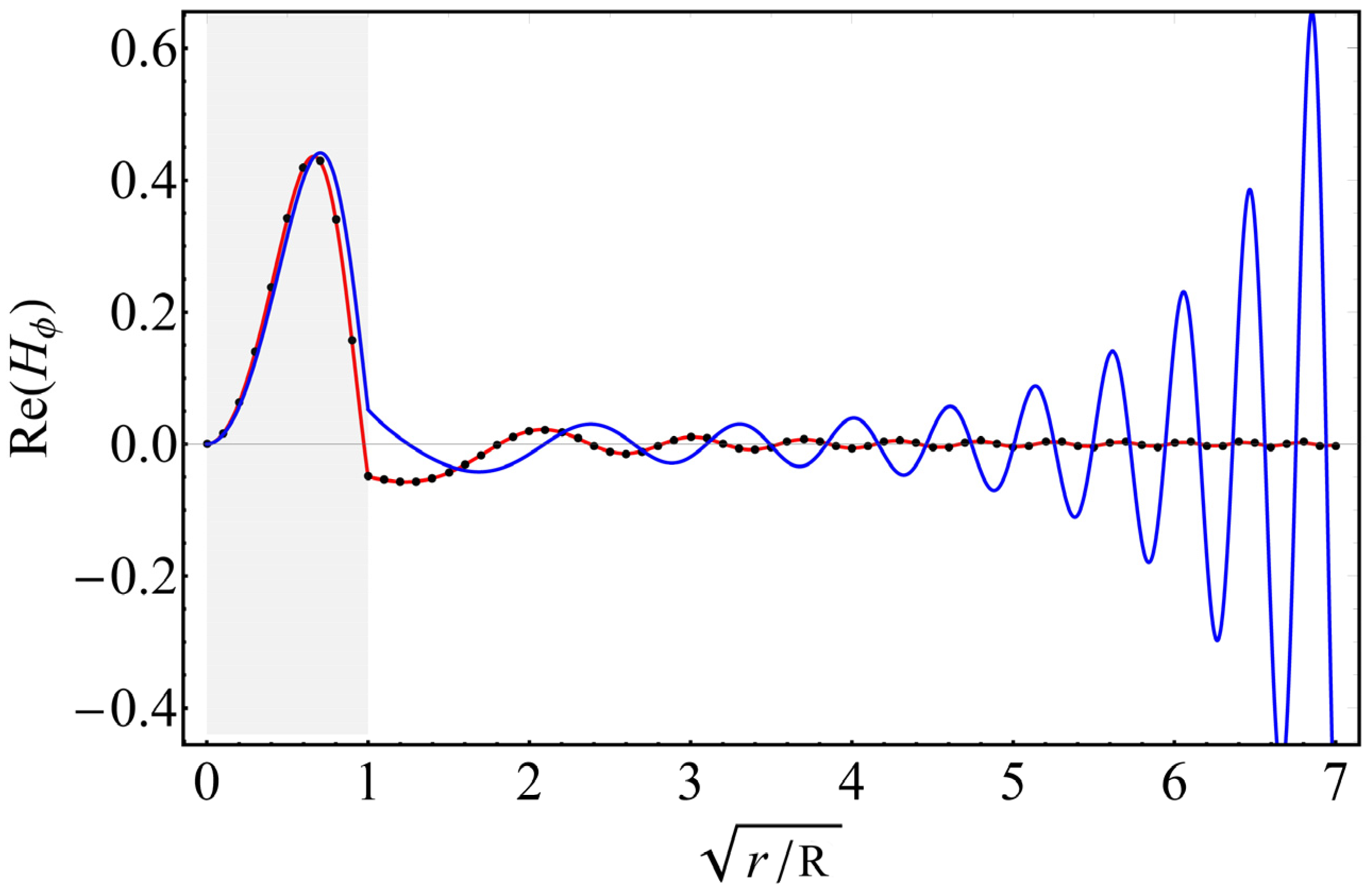
The dispersion Equation (11), along with complex roots, also has real roots, corresponding to perfect nonradiating modes. Figure 1 shows the dependences of on the radius for a perfect nonradiating mode and a usual quasinormal mode with radiation losses.
Figure 1 shows that the quasinormal mode grows exponentially at infinity, while the perfect nonradiating mode goes to zero and has no radiation losses! Inside the resonator, the spatial structures of these modes are similar. It can be seen also from this figure that the spatial structure of the perfect mode does not change practically even in the case of large internal losses (Joule and other). Table 1 shows Q factors of the PTM101 and TM101 modes for a silicon sphere at various wavelengths.
It follows from Table 1 that the Q factors of the perfect modes, even in the case of substantial Joule losses, significantly exceed the Q factors of usual quasinormal modes.
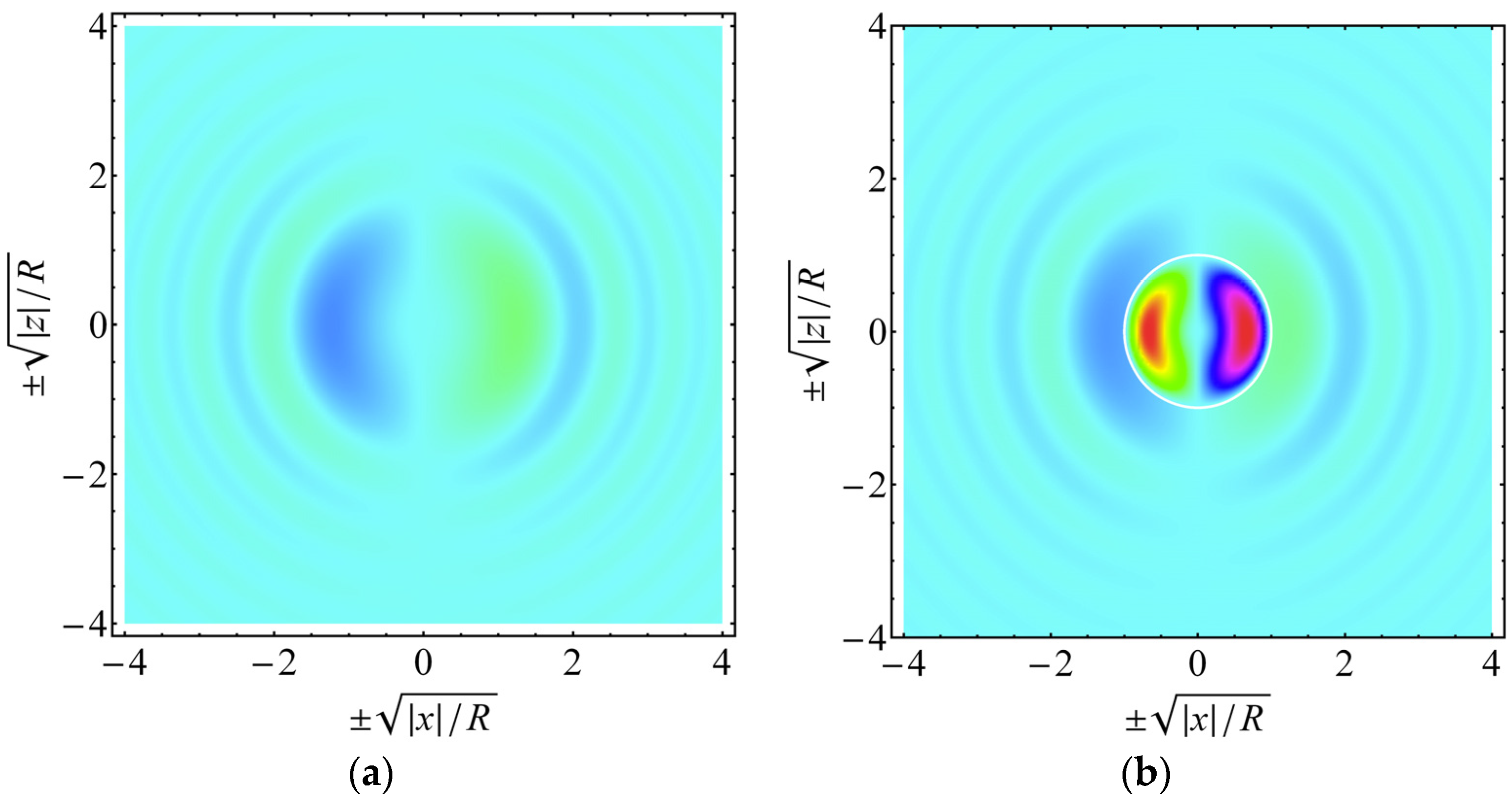
Figure 2 shows the spatial distribution of the excitation field
without any nanoresonator and the full field in the presence of nanoresonator at the frequency of the perfect nonradiating PTM11 mode (see (11)).
Figure 2 shows clearly that the mounting of a nanoparticle into the excitation field (12) does not affect the field outside it; that is, at this frequency, the nanoparticles are invisible.
3.1.2. Manifestation of Perfect Nonradiating Modes in Scattering Experiments
The realization of a spherical standing wave (12) in an experiment is a difficult task, and, therefore, to observe TM perfect nonradiating modes in the sphere, we have performed the Comsol simulations with an incident Bessel beam:
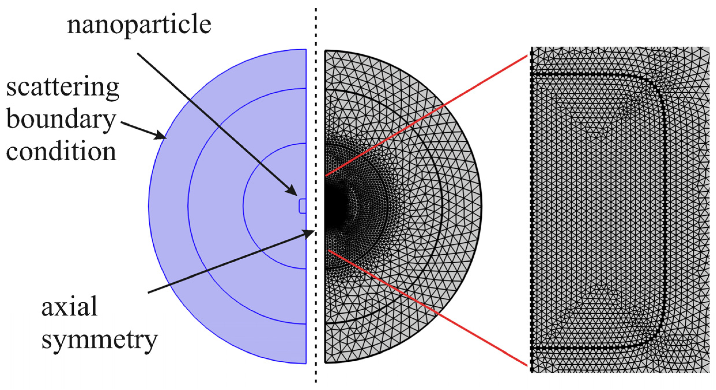
In (13), ρ and z are cylindrical coordinates and α is a conical angle of the Bessel beam. In the vicinity of the origin of coordinates, such a beam approximates the perfect nonradiating mode (12) well. To solve the Maxwell equations within the Comsol Multiphysics software, we used the Radio Frequency interface → Electromagnetic Waves, Frequency Domain → the scattered field formulation. Field (13) was used as a background field. The geometry of the scattering problem and corresponding mesh are shown in Figure 3 and Figure 4.
The results of the simulations are shown in Figure 5.
Figure 5 shows clearly the appearance of an extremely high-quality perfect PTM101 mode in the spectra of a Bessel beam (13) scattered by a sphere. Note that the Q factor of the PTM101 mode is three orders (five orders for standing wave) of magnitude greater than the Q factor of a usual TM101 mode! This figure also shows a significant influence of the spatial structure of the excitation beam on the Q factors of the perfect nonradiating modes.
3.2. TM Perfect Nonradiating Modes in Spheroidall Particles
3.2.1. Analytical Solutions
Nonradiating modes are not a feature of spherical geometry and exist for axisymmetric open dielectric resonators of an arbitrary shape. We have shown rigorously that such modes exist for arbitrary spheroids with semiaxes a and b, having a volume equal to the volume of a sphere of the radius R with a surface described by the equation
The eigenfunctions and eigenvalues of perfect nonradiating modes of such spheroids can be found by expanding the solutions of the Equation (7) over spheroidal functions [34,35]. In the case of TM polarization for a prolate spheroid, a/b > 1, the general axisymmetric solution of Maxwell’s equations [34,35] in the prolate coordinate system (1 < ξ < ∞, −1 < η < 1, 0 < φ < 2π) has the form:
where are the angular spheroidal functions and are the radial spheroidal functions of the first kind, and . For details see Appendix B.
Equating the tangential components of the electric and magnetic fields on the surface of the spheroid (14) and using the orthogonality of angular spheroidal functions, one can find the dispersion equation describing the perfect nonradiating modes:
The dispersion Equation (16) is also valid for an oblate spheroid with the corresponding analytic continuation of spheroidal functions.
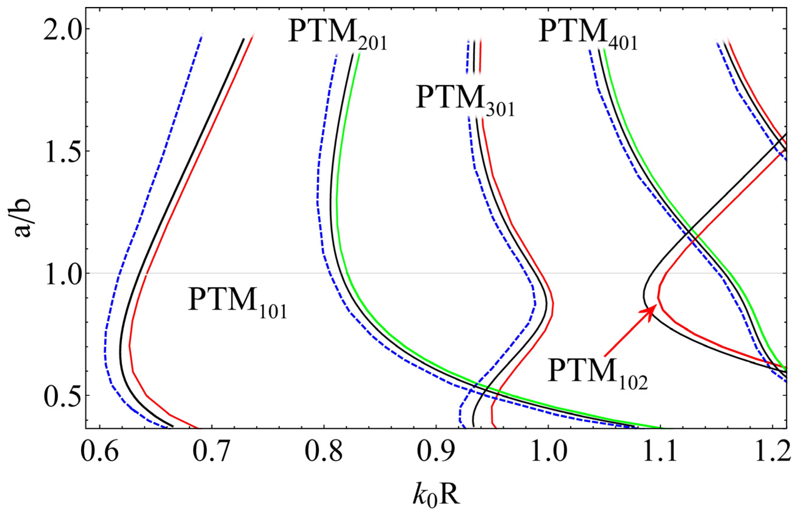
The exact solution of the dispersion Equation (16) for perfect TM modes (PTM) is shown in Figure 6. This figure also shows the dispersion laws of usual TM modes and so-called confined modes [36] with a magnetic field different from zero only inside the nanoparticle and complying with the equations:
and the electric field of the confined modes is zero everywhere.
It can be seen from Figure 6, that for each usual quasinormal mode (blue dashed curves), there are its counterparts in the form of a perfect nonradiating mode (red and green curves), indicating that there are infinitely many perfect nonradiating modes. It should be emphasized here once again that the eigenfrequencies of the perfect nonradiating modes, the solution of (16), are real numbers!
Another interesting fact is that the eigenfrequencies of perfect nonradiating modes are substantially higher than the real parts of frequencies of usual modes . Moreover, it can be argued that the frequencies of confined modes (18), (black curves), appearing in the limit ε → ∞, are always situated between the frequencies of usual and perfect nonradiating modes, . This relationship between frequencies is a manifestation of a very deep connection between confined modes (with fields localized strictly inside the resonator) and perfect nonradiating modes (with fields not localized inside the resonator).
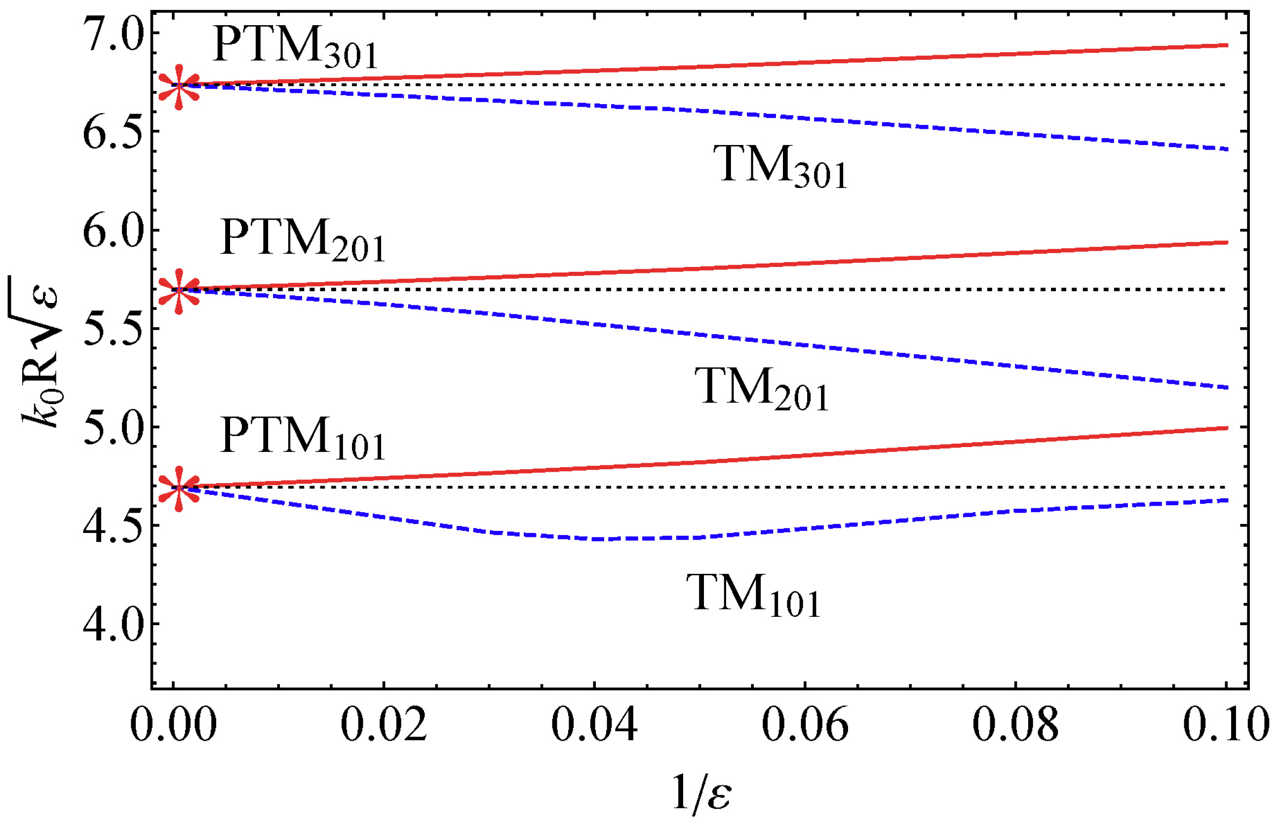
Figure 7 shows the dependence of the frequencies of usual and perfect nonradiating modes on the inverse permittivity.
From Figure 7, it is seen that in the limit ε → ∞, the usual and perfect nonradiating modes merge into confined ones. However, at finite permittivities, this degeneracy is lifted, and confined modes are split into perfect nonradiating modes with infinite Q factors and the usual quasinormal modes with finite Q factors. From Figure 6 and Figure 7 one can clearly see that there is nothing common between the frequencies of perfect nonradiating modes and the frequencies of quasinormal modes.
Such an unambiguous connection between the frequencies of confined modes and perfect nonradiating modes allows us to assert that perfect nonradiating modes with TM polarization definitely exist for any axisymmetric dielectric bodies!
After the eigenvalues are found, the eigenfunctions of the perfect nonradiating modes can be found.
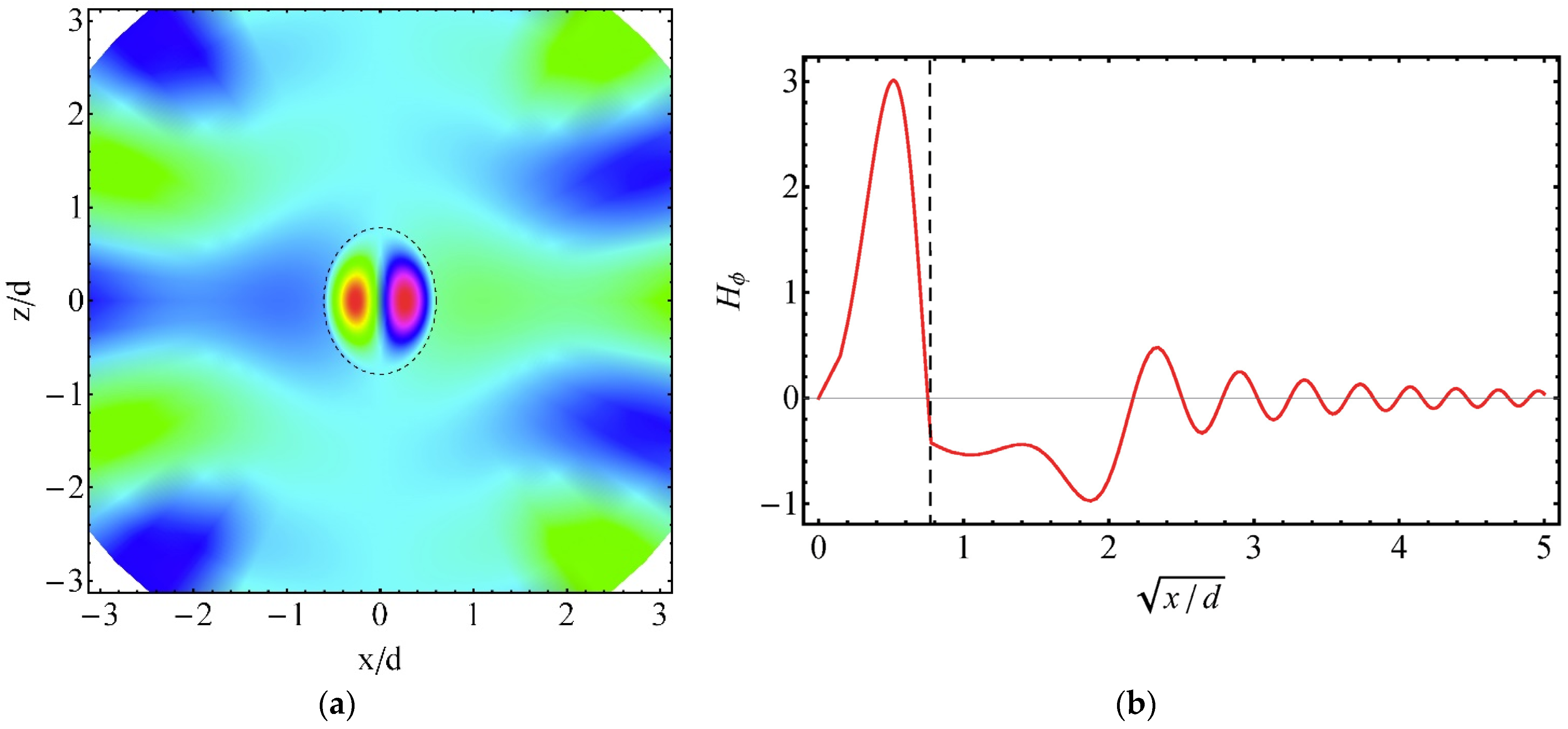
For example, the solution of (15) and (16) for PTM101 mode in a prolate spheroid with ε = 10 and a/b = 1.3 is as follows: k0R = 1.57757, a1 =−7.22705, a3 = 0.0924, a5 = 0.004323, a7 = 0.00019, b1 = 1, b3 = −0.59122, b5 = 1.08884, and b7 = −2.81192 and is shown in Figure 8.
3.2.2. Manifestation of TM Perfect Nonradiating Modes in Scattering Experiments
To demonstrate the great practical importance of the perfect nonradiating modes in spheroids, we have simulated within Comsol Multiphysics software the scattering of an axially symmetric Bessel beam by nanospheroids of different shapes. To observe the even perfect nonradiating modes, we have used an even incident Bessel beam:
In (19), ρ and z are cylindrical coordinates and α is a conical angle of the Bessel beam. In the vicinity of the origin of coordinates, such a beam approximates the perfect nonradiating mode (15) well.
Let us stress that the Comsol simulations are fully independent of our analytical results (16) and (17) and fully confirm them.
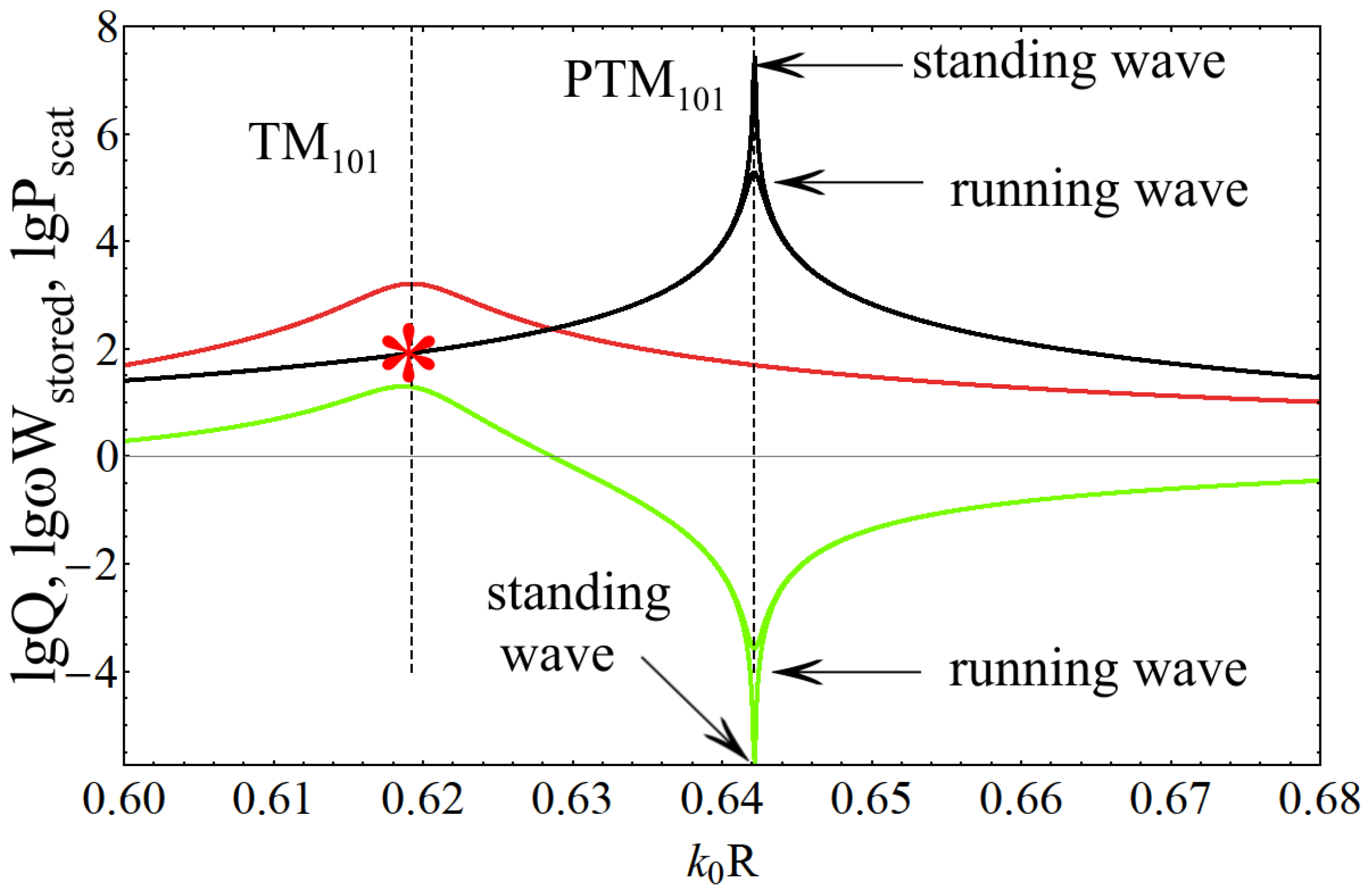
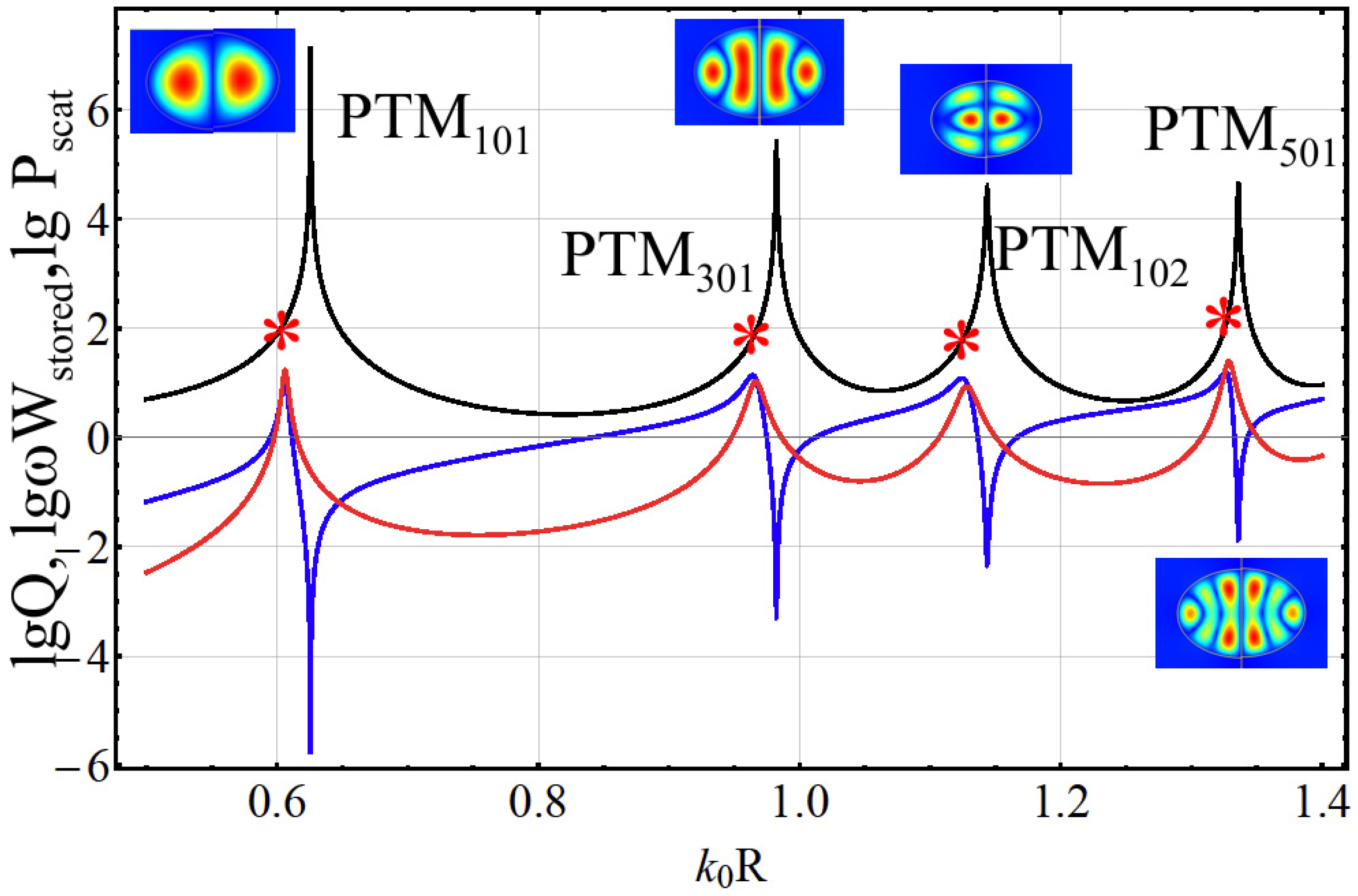
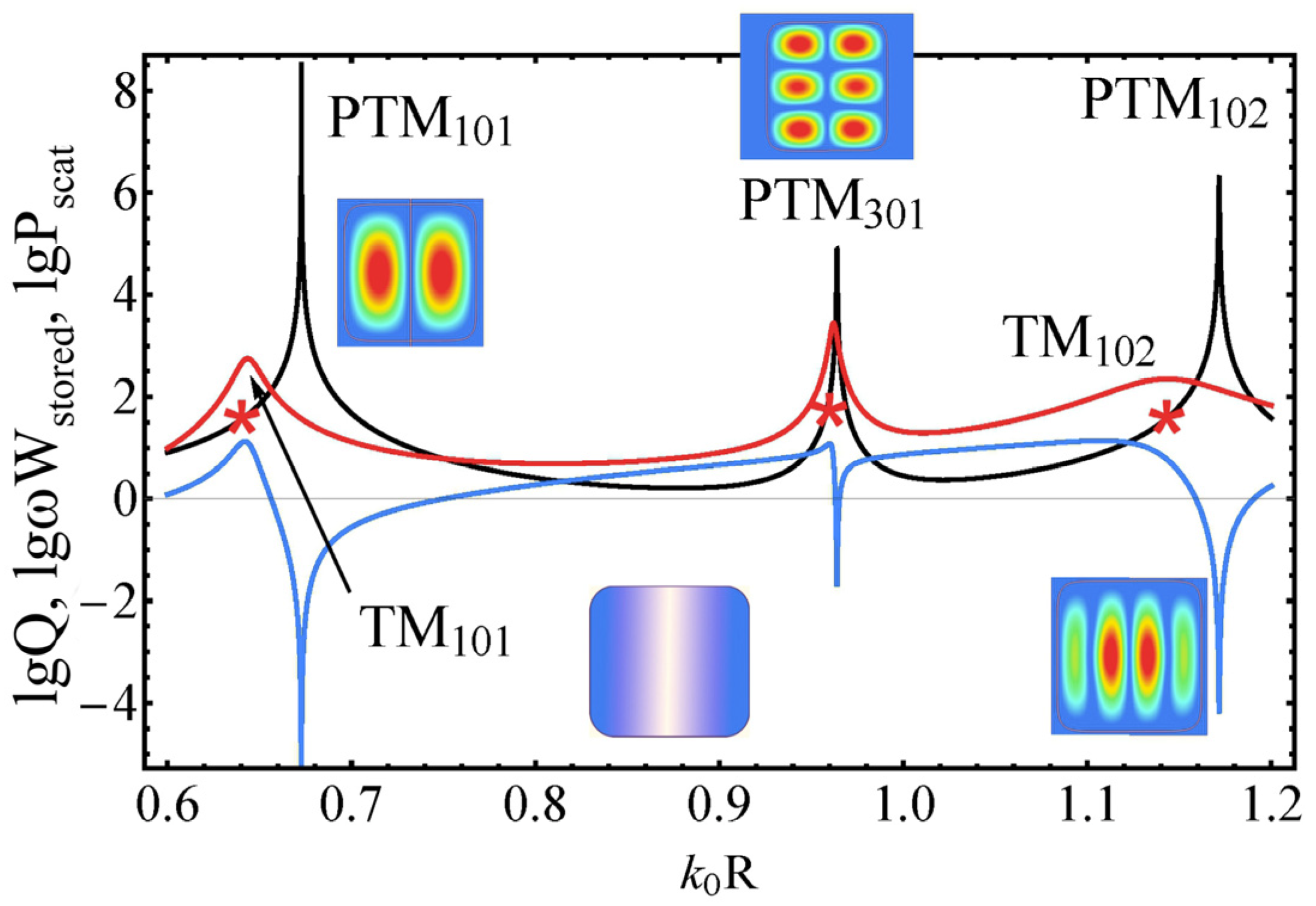
In Figure 9 one can see the simulated dependence of scattered power Pscat, stored energy Wstored, and the generalized radiation quality factor Q = ωWstored/Pscat, on the size parameter of nanospheroids for aspect ratio a/b = 0.7.
Figure 9 clearly shows the presence of perfect nonradiating modes, having Q factors significantly higher than the Q factors of usual quasinormal modes. It can be seen from this figure that, upon excitation (19), all the maxima of the generalized Q factor are due to the perfect nonradiating modes shown in Figure 6 and Figure 7. In this case, the Q factors of usual modes (shown by asterisks) are several orders of magnitude lower than the Q factors of perfect nonradiating modes! Moreover, smart optimization of the excitation beam [27] makes it possible to increase the Q factor of perfect nonradiating modes almost unlimitedly.
3.3. TE Perfect Nonradiating Modes in Spheroidall Particles
3.3.1. Analytical Solutions
In this case, the only nonzero component of the electric field can be written in the form:
Equating the tangential components of the electric and magnetic fields on the surface of the spheroid (14) and using the orthogonality of angular spheroidal functions, one can find the dispersion equation describing the TE perfect nonradiating modes:
which differs from the dispersion Equation (16) only by the absence of ε in the parenthesis.
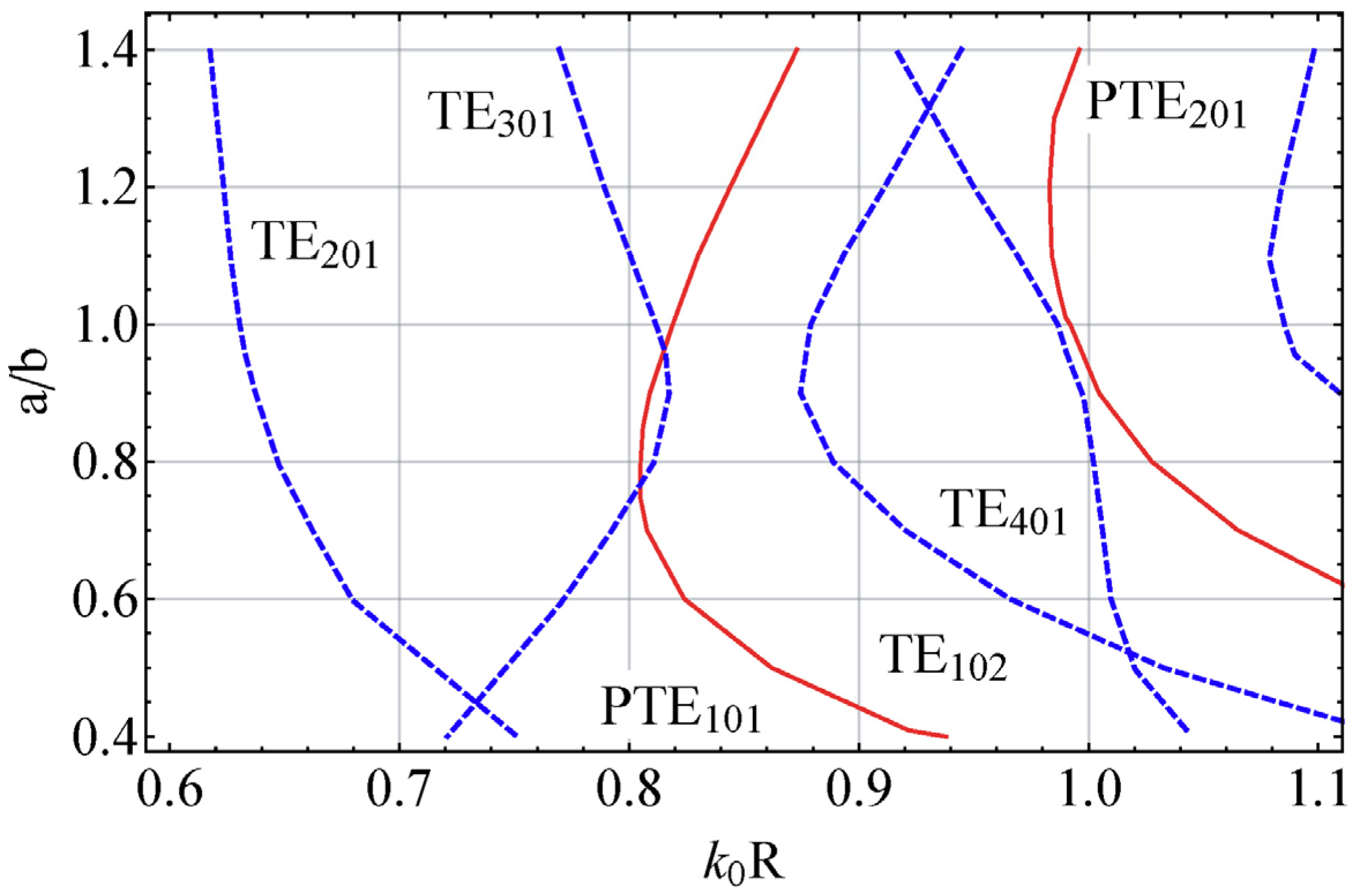
The exact solution of the dispersion Equation (21) for perfect TE modes (PTE) is shown in Figure 10.
From Figure 10 and the structure of the dispersion Equation (21), it follows that the number of perfect nonradiating modes with TE polarization is infinite, as in the case of TM polarization.
It is clearly seen from Figure 10, that the frequencies of the perfect nonradiating modes with TE polarization are located very far from the frequencies of the usual TE modes of similar symmetry, indicating that there is no connection between usual and perfect modes.
3.3.2. Manifestation of TE Perfect Nonradiating Modes in Scattering Experiments
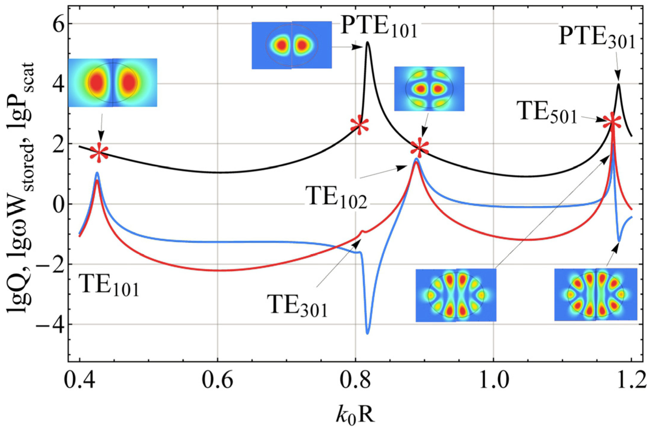
Demonstration of the existence of TE perfect nonradiating modes in scattering spectra is more complicated in comparison with the TM case since perfect modes with TE polarization are not confined modes [36] in the limit ε → ∞. In addition, the frequencies of perfect PTEn,0,1 modes turn out to be close to the frequencies of usual TEn+2,0,1 modes. Therefore, to demonstrate perfect nonradiating TE modes, an incident beam should not excite the usual nearby modes. In particular, to demonstrate the existence of the PTE101 mode (see Figure 11), it is necessary to suppress the excitation of the usual TE301 mode by using an exciting field of the form:
In (22), r and θ are spherical coordinates and jn(x) and are the spherical Bessel functions and the Legendre polynomial, correspondingly.
Figure 11 clearly shows the presence of the perfect nonradiating modes, having Q factors significantly higher than the Q factors of usual modes. Moreover, smart optimization of the excitation beam [27] makes it possible to increase the Q factor of the perfect nonradiating modes unlimitedly (with the neglect of Joule losses in the nanoparticle material, of course).
3.4. TM Perfect Nonradiating Modes in Cylindrical Particles
We have not yet succeeded in finding an analytical solution for perfect nonradiating modes in a dielectric cylinder of a finite height. However, proceeding from the very plausible hypothesis that the existence of perfect modes is associated with the existence of confined modes, we have found the frequencies of perfect nonradiating modes by the Comsol simulation of the scattering of a Bessel beam
by a superspheroid with the surface described by the equation:
For t = 2, this is a sphere. For t = ∞, this is a cylinder with the diameter Dcyl = 2a (∞) and the height Hcyl = 2c (∞).
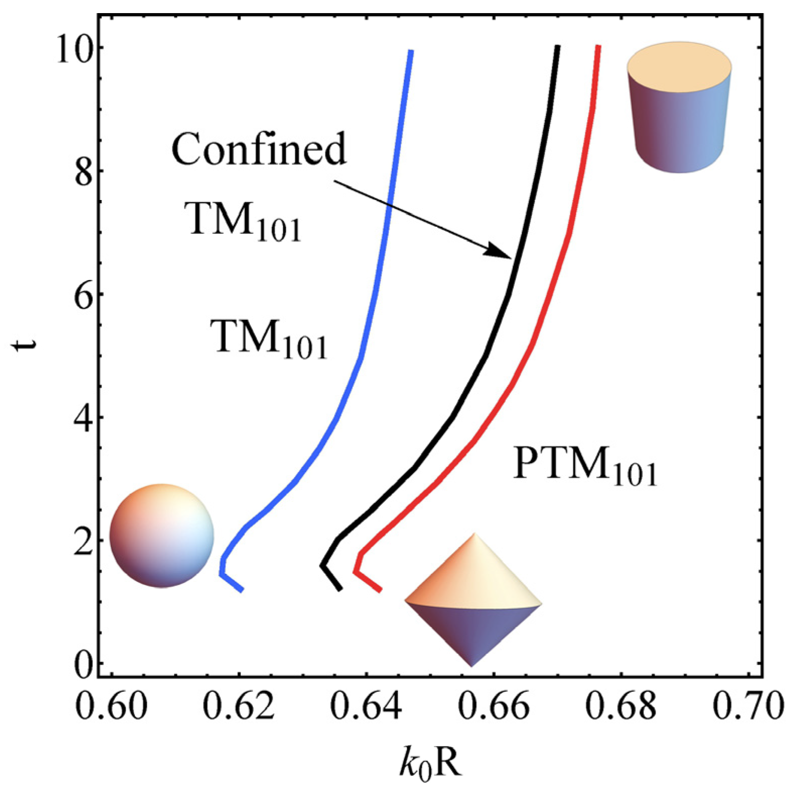
The results of the Comsol simulation are shown in Figure 12.
It is clearly seen from Figure 12 that the frequencies of the perfect nonradiating modes with TM polarization in superspheroids are located very far from the frequencies of the usual modes of similar symmetry, indicating that there is no connection between the usual and perfect modes.
In Figure 13, one can see the dependence of scattered power, stored energy, and generalized Q factor on the size parameter k0R of a superspheroid with shape parameter t = 8, when excited by a Bessel beam (23).
Figure 13 shows that all the maxima of the generalized Q factor with the excitation (23) are due to perfect nonradiating modes, with Q factors of several orders of magnitude higher than the Q factors of usual modes.
4. Discussion
Above, as an example, perfect nonradiating PTM and PTE modes in dielectric spheroidal nanoparticles are considered. However, this approach can be directly generalized to waveguides [37]. Moreover, this approach can be directly generalized to nanoparticles made from double negative (DNG) or chiral metamaterials.
The system of equations for finding perfect nonradiating modes without boundary conditions at infinity (a generalization of the system (7)) in this case has the form:
where E and H are the inductions and the strengths of electric and magnetic fields, correspondingly, ε and μ are the permittivity and the permeability of the chiral medium, and η is the dimensional parameter of chirality. The solution of the system (25) in the case of a chiral spherical resonator can be found using the method described in [38].
However, the existence of perfect nonradiating modes for non-symmetric nanoparticles is still questionable.
Thus, we have put forward the hypothesis of the existence of perfect nonradiating eigenmodes of light in dielectric nanoparticles. These modes are the exact solutions of sourceless Maxwell equations. We have shown rigorously that in the case of axisymmetric particles, such modes always exist and arise at frequencies somewhat higher than the resonance frequencies of usual quasinormal modes.
In a spherical case, the problem of finding perfect nonradiating modes can be reduced to the scattering problem, where it is required to find the parameters of the incident (converging) and scattered (diverging) spherical waves, at which the total energy flux is zero. However, this approach is difficult to generalize in the case of 3D nanoparticles of a more complex shape, since, in this case, the field of the perfect nonradiating mode cannot be represented as a superposition of a priori known converging and diverging waves.
Another approach for finding perfect nonradiating modes can be the analysis of the spatial structure of two arbitrary solutions of sourceless Maxwell equations, E1, H1, and E2, H2 in free unbounded spaces with permittivities ε1, ε2 in order to find a surface S where the tangential components of the fields are equal, . If such a surface can be found, then it can be considered as the surface of a dielectric particle. As a result, if the interior of such a surface is replaced by a substance with a permittivity of ε1, then the field E2 outside this surface will not change, that is, the particle will be invisible (see Figure 2).
As can be seen from the above, perfect nonradiating modes possess fully different physics than quasinormal modes and have no analogs. In particular, they differ from the so-called anapole states [17,20,21,22,23,24,25] in that their field outside the particle is different from zero and has a well-defined expansion over spherical (5) or spheroidal (15) harmonics. These modes also differ from high-Q supercavity modes or quasi-BIC states because perfect modes do not radiate at all. The perfect modes are closest to strange Neumann–Wigner modes [29], but unlike the latter, the optical potential of a nanoparticle, , differs from the vacuum value only in a bounded region of space, fundamentally distinguishing perfect nonradiating modes from Neumann–Wigner modes [29]. In addition, perfect nonradiating modes are vector ones in contrast to the scalar wave functions in quantum mechanics.
Due to the extremely small scattered power and unlimited radiation Q factors, our finding paves the way for the development of new nano-optical devices, with a high concentration of field inside nanoparticles and extremely small radiative losses, including low threshold nanolasers, biosensors, parametric amplifiers, and nanophotonics quantum circuits.
Funding
This research was funded by the Russian Foundation for Basic Research, grant number 20-12-50136.
Institutional Review Board Statement
Not applicable.
Data Availability Statement
Not applicable.
Conflicts of Interest
The authors declare no conflict of interest.
Appendix A
Theory of Perfect Nonradiating Modes in Dielectric Sphere
In the axisymmetric nonmagnetic case m = 0, there is no dependence on φ, and only the azimuthal component of the magnetic field Hφ is nonzero, so inside the sphere one can write [39]
Here, for the spherical harmonics with m = 0, we have used their expression in terms of the Legendre polynomials, Yn0(θ,φ) = Pn(cosθ), k1 = √εk0, where k0 is the wave number in the vacuum, jn are the spherical Bessel functions, and A is the amplitude of the perfect nonradiating mode inside the sphere. Time dependence, ~, is assumed everywhere.
Outside the sphere (in a vacuum, ε = 1), we are looking for a solution in exactly the same nonsingular form (and this is a novelty!) with the replacement k1 →k0:
In (A2), B is the amplitude of a perfect nonradiative mode outside the sphere.
On the boundary of the sphere r = R, the tangential components of the fields must be continuous, that is, for any 0 < θ < π, the following conditions must be met:
Using the orthogonality of the Legendre polynomials, the system of equations that determine the eigenfrequencies of perfect nonradiating modes can be written as:
The nontrivial solutions of (A4), i.e., the perfect nonradiating modes, exist if the determinant of (A4) is equal to zero:
where X = k0R is a size parameter.
For each ε > 1 and n > 1, Equation (A5) has an infinite number of real roots, indicating the existence of perfect nonradiating modes, and where the field distributions take the form:
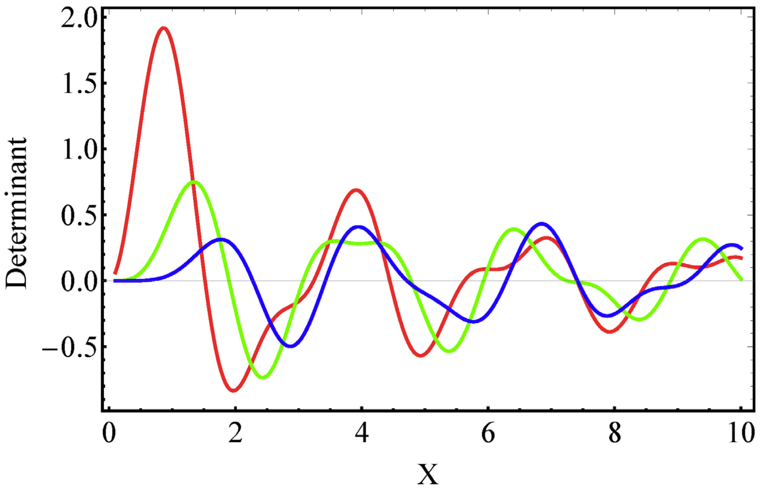
As an example, Figure A1 shows the dependencies of the left side of (A5) on the size parameter X for a sphere with permittivity ε = 10.
Figure A1.
Dependences of the left side of (A5) on the size parameter X = k0R for a sphere with permittivity ε = 10 for n = 1 (red), n = 2 (green), and n = 3 (blue).
Figure A1.
Dependences of the left side of (A5) on the size parameter X = k0R for a sphere with permittivity ε = 10 for n = 1 (red), n = 2 (green), and n = 3 (blue).

Figure A1 shows an infinite set of real roots that correspond to the perfect nonradiating modes.
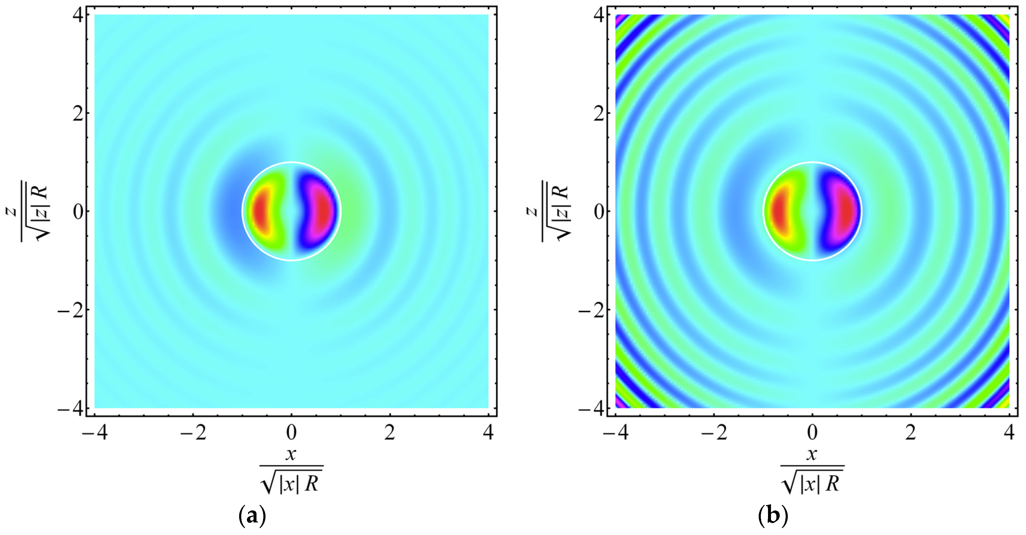
The dependence of the radial part of usual and perfect non-radiating modes on the radius is shown in Figure 1 of the article. Figure A2 shows the spatial distribution of ReHφ in the perfect nonradiating mode and the usual mode in a sphere with ε = 10.
Figure A2.
Spatial distribution of ReHφ in (a) the perfect nonradiating PTM101 mode (k0R = 1.51893) and (b) the usual TM101 mode (k0R = 1.35715−0.160978 i) in a sphere of the radius R with ε = 10.
Figure A2.
Spatial distribution of ReHφ in (a) the perfect nonradiating PTM101 mode (k0R = 1.51893) and (b) the usual TM101 mode (k0R = 1.35715−0.160978 i) in a sphere of the radius R with ε = 10.

It is clearly seen from Figure A2 that the perfect mode exists, has a sensible spatial distribution, and decreases at infinity, while the usual quasinormal mode increases exponentially at infinity.
Thus, the existence of the perfect nonradiating modes in the dielectric sphere has been rigorously proved.
Appendix B
Appendix B.1. Theory of Perfect Nonradiating Modes in Dielectric Spheroids
Apparently, perfect nonradiating modes exist for axisymmetric bodies of an arbitrary shape. It is precisely shown below that such modes exist for arbitrary spheroids with semiaxes a and b, having a volume equal to the volume of a sphere of the radius R and a surface described by the equation:
where t = a/b. For t < 1, we have an oblate spheroid, and for t > 1, it is an elongated one.
The eigenvalues and eigenfunctions of the perfect nonradiating modes of such spheroids can be found by solving sourceless Maxwell equations in the prolate spheroidal coordinates ξ, η, φ [34,35]. In these coordinates, the surface of the spheroid (A7) is determined by the condition:
In spheroidal coordinates, the variables can be separated, and solutions of Maxwell’s equations can be represented as an expansion over spheroidal wave functions.
Appendix B.2. TM Polarization, Non-Magnetic Case
In the case of TM polarization, for a single nonzero component of the magnetic field, one can write
where are the angular spheroidal functions and are the radial spheroidal functions of the first kind [34].
The tangential component of the electric field looks like:
inside nanoparticles, , and
everywhere, . In (A10) and (A11) and elsewhere, .
After multiplication by angular harmonics, integration over η, and application of the orthogonality condition for angular spheroidal functions,
the conditions for the continuity of the magnetic and electric fields at the spheroid boundary ξ = ξ0 take the form:
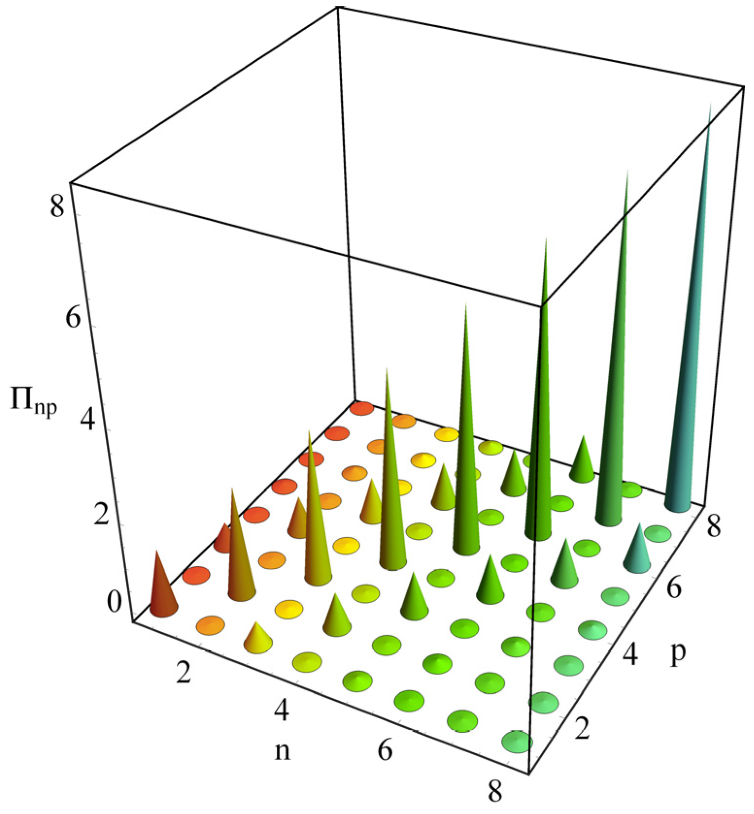
Figure A3 shows the dependence of the overlap integral ∏n,p(c1,c0) of angular spheroidal functions on the indices n, p.
Figure A3 shows that:
- Only modes with the same parity interact with each other;
- For each mode, interaction is essential only with the nearest modes of the same parity, 2k⇔2(k ± 1); 2k + 1⇔2(k ± 1) + 1.
This circumstance simplifies calculations since matrices of finite dimension 3 × 3 can be used to calculate eigenfrequencies with high accuracy.
Eliminating an from (A13) and (A14), we obtain a homogeneous system of equations for the coefficients bp, determining the magnetic field outside the particle:
The compatibility condition of (A15) allows one to find the modes and eigenfrequencies of the perfect nonradiating modes shown in Figure 6 and Figure 7 of the article.
Figure A3.
Dependence of the overlap integral of angular spheroidal functions in an elongated spheroid ∏n,p(c1,c0) on indices. c1 = 4, c0 = c1/ = 0.5657, ε = 50.
Figure A3.
Dependence of the overlap integral of angular spheroidal functions in an elongated spheroid ∏n,p(c1,c0) on indices. c1 = 4, c0 = c1/ = 0.5657, ε = 50.

Appendix B.3. TE Polarization, Non-Magnetic Case
In this case, the only nonzero component of the electric field can be written in the form:
Repeating the reasoning for TM polarization (see Appendix B.2) for the coefficients bp, determining the electric field outside the particle, we obtain a homogeneous system of equations:
that differs from the dispersion Equation (A15) only by the absence of ε in the parenthesis.
References
- Novotny, L.; Van Hulst, N. Antennas for light. Nat. Photon. 2011, 5, 83–90. [Google Scholar] [CrossRef]
- Biagioni, P.; Huang, J.S.; Hecht, B. Nanoantennas for visible and infrared radiation. Rep. Prog. Phys. 2012, 75, 024402. [Google Scholar] [CrossRef] [PubMed] [Green Version]
- Tiguntseva, E.; Koshelev, K.; Furasova, A.; Tonkaev, P.; Mikhailovskii, V.; Ushakova, E.V.; Baranov, D.G.; Shegai, T.; Zakhidov, A.A.; Kivshar, Y.; et al. Room-Temperature Lasing from Mie-Resonant Nonplasmonic Nanoparticles. ACS Nano 2020, 14, 8149. [Google Scholar] [CrossRef] [PubMed]
- Mylnikov, V.; Ha, S.T.; Pan, Z.; Valuckas, V.; Paniagua-Dominguez, R.; Demir, H.V.; Kuznetsov, A.I. Lasing Action in Single Subwavelength Particles Supporting Supercavity Modes. ACS Nano 2020, 14, 7338. [Google Scholar] [CrossRef] [PubMed]
- Zheng, K.; Zhang, Z.; Qin, F.; Xu, Y. Invisible Mie scatterer. Opt. Lett. 2021, 46, 5248–5251. [Google Scholar] [CrossRef]
- Liu, Z.; Zhou, Y.; Guo, Z.; Zhao, X.; Luo, M.; Li, Y.; Wu, X. Ultrahigh Q-Guided Resonance Sensor Empowered by Near Merging Bound States in the Continuum. Photonics 2022, 9, 852. [Google Scholar] [CrossRef]
- Barreda, A.I.; Sanz, J.M.; Gonzalez, F. Using linear polarization for sensing and sizing dielectric nanoparticles. Opt. Express 2015, 23, 9157. [Google Scholar] [CrossRef]
- García-Cámara, B.; Gómez-Medina, R.; Sáenz, J.J.; Sepúlveda, B. Sensing with magnetic dipolar resonances in semiconductor nanospheres. Opt. Express 2013, 23, 23007. [Google Scholar] [CrossRef] [Green Version]
- Barreda, A.; Vitale, F.; Minovich, A.; Ronning, C.; Staude, I. Applications of Hybrid Metal-Dielectric Nanostructures: State of the Art. Adv. Photonics Res. 2022, 3, 2100286. [Google Scholar] [CrossRef]
- Grinblat, G.; Li, Y.; Nielsen, M.P.; Oulton, R.F.; Maier, S.A. Efficient third harmonic generation and nonlinear subwavelength imaging at a higher-order anapole mode in a single germanium nanodisk. ACS Nano 2017, 11, 953–960. [Google Scholar] [CrossRef]
- Hsu, C.W.; Zhen, B.; Lee, J.; Chua, S.-L.; Johnson, S.G.; Joannopoulos, J.D.; Soljačic, M. Observation of trapped light within the radiation continuum. Nature 2013, 499, 188. [Google Scholar] [CrossRef] [PubMed] [Green Version]
- Hsu, C.; Zhen, B.; Stone, A.; Joannopoulos, J.D.; Soljačic, M. Bound states in the continuum. Nat. Rev. Mater. 2016, 1, 16048. [Google Scholar] [CrossRef] [Green Version]
- Koshelev, K.; Favraud, G.; Bogdanov, A.; Kivshar, Y.; Fratalocchi, A. Nonradiating photonics with resonant dielectric nanostructures. Nanophotonics 2019, 8, 725. [Google Scholar] [CrossRef]
- Carletti, L.; Koshelev, K.; de Angelis, C.; Kivshar, Y. Giant nonlinear response at the nanoscale driven by bound states in the continuum. Phys. Rev. Lett. 2018, 121, 33903. [Google Scholar] [CrossRef] [Green Version]
- Rybin, M.V.; Koshelev, K.L.; Sadrieva, Z.F.; Samusev, K.B.; Bogdanov, A.A.; Limonov, M.F.; Kivshar, Y.S. High-Q supercavity modes in subwavelength dielectric resonators. Phys. Rev. Lett. 2017, 119, 243901. [Google Scholar] [CrossRef] [Green Version]
- Odit, M.; Koshelev, K.; Gladyshev, S.; Ladutenko, K.; Kivshar, Y.; Bogdanov, A. Observation of supercavity modes in subwavelength dielectric resonators. Adv. Mater. 2021, 33, 2003804. [Google Scholar] [CrossRef]
- Zel’dovich, Y.B. Electromagnetic interaction with parity violation. JETP 1957, 6, 1184. [Google Scholar]
- McLean, J.S.; Foltz, H. The Relationship between Cartesian Multipoles and Spherical Wavefunction Expansions with Application to Wireless Power Transfer. In Proceedings of the Antenna Measurement Techniques Association Symposium (AMTA), Newport, RI, USA, 2–5 November 2020; pp. 1–6. [Google Scholar]
- Radescu, E., Jr.; Vaman, G. Cartesian Multipole Expansions and Tensorial Identities. Prog. Electromagn. Res. B 2012, 36, 89. [Google Scholar] [CrossRef] [Green Version]
- Yang, Y.; Bozhevolnyi, S.I. Nonradiating anapole states in nanophotonics: From fundamentals to applications. Nanotechnology 2019, 30, 204001. [Google Scholar] [CrossRef]
- Manna, U.; Sugimoto, H.; Eggena, D.; Coe, B.; Wang, R.; Biswas, M.; Fujii, M. Selective excitation and enhancement of multipolar resonances in dielectric nanospheres using cylindrical vector beams. J. Appl. Phys. 2020, 127, 033101. [Google Scholar] [CrossRef]
- Parker, J.A.; Sugimoto, H.; Coe, B.; Eggena, D.; Fujii, M.; Scherer, N.F.; Gray, S.K.; Manna, U. Excitation of Nonradiating Anapoles in Dielectric Nanospheres. Phys. Rev. Lett. 2020, 124, 097402. [Google Scholar] [CrossRef] [PubMed]
- Luk’yanchuk, B.; Paniagua-Domínguez, R.; Kuznetsov, A.I.; Miroshnichenko, A.E.; Kivshar, Y.S. Hybrid anapole modes of high-index dielectric nanoparticles. Phys. Rev. A. 2017, 95, 063820. [Google Scholar] [CrossRef]
- Wei, L.; Xi, Z.; Bhattacharya, N.; Urbach, H.P. Excitation of the radiationless anapole mode. Optica 2016, 3, 799. [Google Scholar] [CrossRef] [Green Version]
- Lu, Y.; Xu, Y.; Ouyang, X.; Xian, M.; Cao, Y.; Chen, K.; Li, X. Cylindrical vector beams reveal radiationless anapole condition in a resonant state. Opto-Electron. Adv. 2021, 5, 210076. [Google Scholar] [CrossRef]
- Diaz-Escobar, E.; Bauer, T.; Pinilla-Cienfuegos, E.; Barreda, Á.I.; Griol, A.; Kuipers, L.; Martínez, A. Radiationless anapole states in on-chip photonics. Light Sci. Appl. 2021, 10, 204. [Google Scholar] [CrossRef]
- Klimov, V. Manifestation of extremely high-Q pseudo-modes in scattering of a Bessel light beam by a sphere. Opt. Lett. 2020, 45, 4300. [Google Scholar] [CrossRef]
- Bohren, C.; Huffmann, D. Absorption and Scattering of Light by Small Particles; John Wiley: New York, NY, USA, 1983. [Google Scholar]
- von Neumann, J.; Wigner, E.P. Uber merkwiirdige diskrete Eigenwerte. Phys. Z. 1929, 30, 465. [Google Scholar]
- Arai, M.; Uchiyama, J. On the von Neumann and Wigner Potentials. J. Differ. Equ. 1999, 157, 348. [Google Scholar] [CrossRef] [Green Version]
- Schinke, C.; Peest, P.C.; Schmidt, J.; Brendel1, R.; Bothe, K.; Vogt, M.R.; Kröger, I.; Winter, S.; Schirmacher, A.; Lim, S.; et al. Uncertainty analysis for the coefficient of band-to-band absorption of crystalline silicon. AIP Adv. 2015, 5, 67168. [Google Scholar] [CrossRef] [Green Version]
- Weiting, F.; Yixun, Y. Temperature effects on the refractive index of lead telluride and zinc selenide. Infrared Phys. 1990, 30, 371. [Google Scholar] [CrossRef]
- Krishnamoorthy, H.N.S.; Adamo, G.; Yin, J.; Savinov, V.; Zheludev, N.I.; Soci, C. Infrared dielectric metamaterials from high refractive index chalcogenides. Nat. Comm. 2020, 11, 1692. [Google Scholar]
- Meixner, J.; Schäfke, F.W. Mathieusche Funktionen und Sphäroidfunktionen mit Anwendungen auf Physikalische und Technische Probleme; Grundlehren der mathematischen Wissenschaften; Springer: Berlin/Heidelberg, Germany, 1954; Volume 71, 432p. [Google Scholar]
- Li, L.-W.; Kang, X.-K.; Leong, M.-S. Spheroidal Wave Functions in Electromagnetic Theory; John Wiley & Sons, Inc.: Hoboken, NJ, USA, 2002. [Google Scholar]
- van Bladel, J. On the resonances of a dielectric resonator of very high permittivity. IEEE Trans. Microw. Theory Tech. 1975, MTT-23, 199–208. [Google Scholar] [CrossRef]
- Klimov, V.V.; Guzatov, D.V. Perfect Nonradiating Modes in Dielectric Nanofiber with Elliptical Cross-Section. Available online: https://arxiv.org/abs/2204.13327v2 (accessed on 2 May 2022).
- Guzatov, D.V.; Klimov, V.V. The influence of chiral spherical particles on the radiation of optically active molecules. New J. Phys. 2012, 14, 123009. [Google Scholar] [CrossRef]
- Stratton, J.A. Electromagnetic Theory; McGraw-Hill Book Company: New York, NY, USA; London, UK, 1941; 557p. [Google Scholar]
Figure 1.
The dependence of on the radius for the usual TM101 mode (blue, k0R = 1.22332–0.12557 i, ε = 12), for the perfect nonradiating PTM101 mode ((10), red, k0R = 1.36687, ε = 12) and for the perfect nonradiating PTM101 mode in a sphere with large losses ((10), black dots, k0R = 1.36568–0.0323 i, ε = 12 + 0.5 i).

Figure 2.
(a) Spatial distribution of the excitation field (12) at the frequency of the perfect nonradiating mode PTM11 and (b) full field (10) in the presence of nanoparticle (n = 1, k0R = 1.36687, ε = 12).
Figure 2.
(a) Spatial distribution of the excitation field (12) at the frequency of the perfect nonradiating mode PTM11 and (b) full field (10) in the presence of nanoparticle (n = 1, k0R = 1.36687, ε = 12).

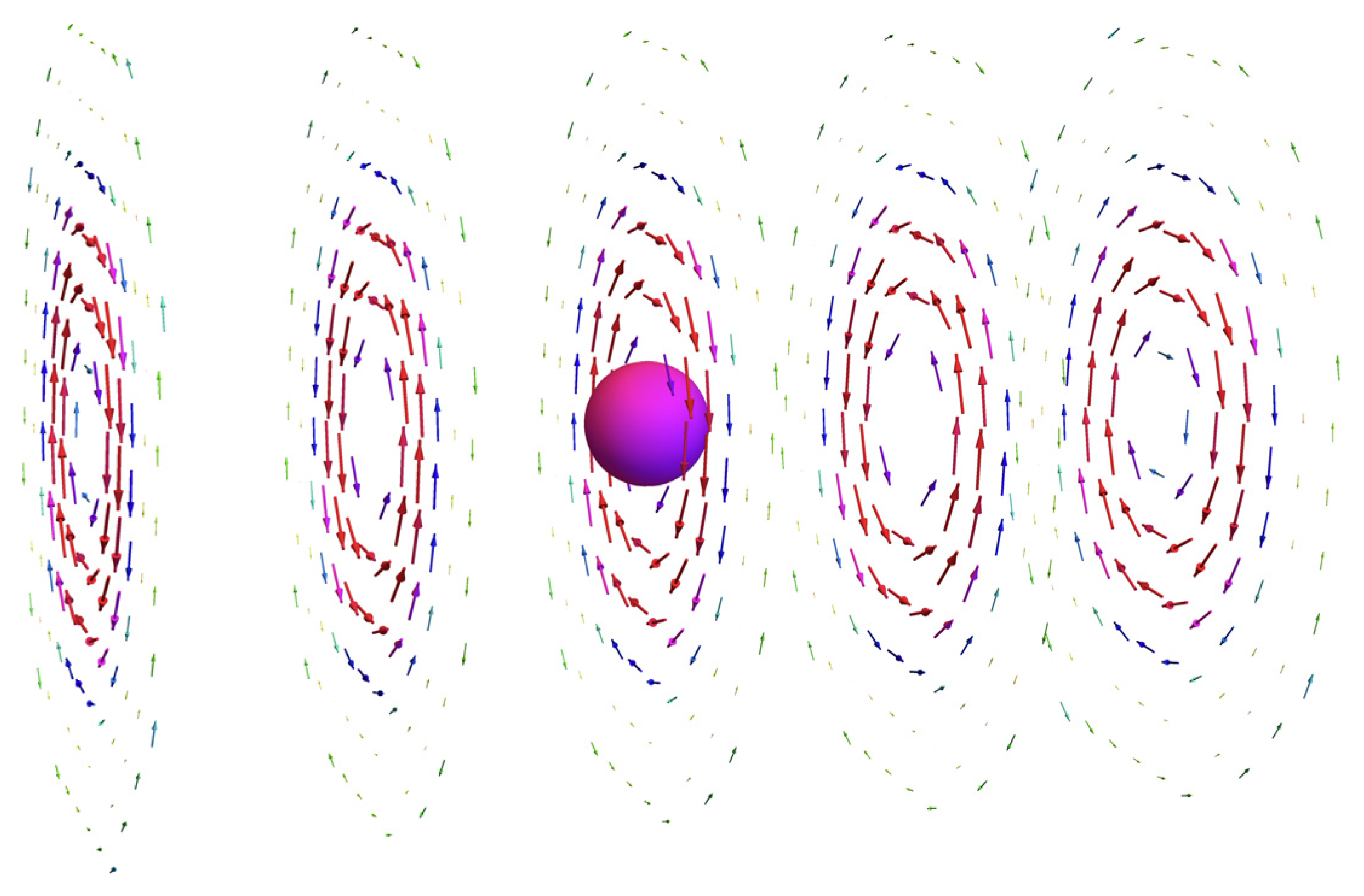
Figure 3.
A nanoparticle inside an incident Bessel beam (13). Arrows show ReHφ distribution.

Figure 4.
Geometry and a mesh of the Comsol simulation.

Figure 5.
The dependence of scattered power Pscat (green), stored energy Wstored (red), and generalized radiation quality factor Q = ωWstored/Pscat (black) on the size parameter of a sphere obtained within the Comsol simulation. TM excitation (13), α = atan (2), ε = 50 (Bi2Te3). The asterisk on the red curve shows the Q factor value of the TM101 mode.

Figure 6.
Perfect nonradiating TM modes (PTM) of spheroids with ε = 50 (Bi2Te3) as a function of the size parameter k0R and the spheroid aspect ratio, a/b. Red and green curves stand for odd and even perfect nonradiating modes, blue dashed lines correspond to usual quasinormal modes. Black curves show the frequencies of confined modes (18), ωn,confined = k0nc.

Figure 7.
Dependence of for usual (blue dashed curves, TM) and perfect nonradiating modes (red curves, PTM) on 1/ε for a prolate spheroid with a/b = 1.3. The red asterisks and black dashed lines indicate confined modes (18).
Figure 7.
Dependence of for usual (blue dashed curves, TM) and perfect nonradiating modes (red curves, PTM) on 1/ε for a prolate spheroid with a/b = 1.3. The red asterisks and black dashed lines indicate confined modes (18).

Figure 8.
(a) Spatial distribution of Hφ (x,z) and (b) the dependence of Hφ (x,z = 0) on x (right) in the PTM101 mode in a prolate spheroid with ε = 10, k0R = 1.57757, k0d = 2.4, a/b = 1.3.
Figure 8.
(a) Spatial distribution of Hφ (x,z) and (b) the dependence of Hφ (x,z = 0) on x (right) in the PTM101 mode in a prolate spheroid with ε = 10, k0R = 1.57757, k0d = 2.4, a/b = 1.3.

Figure 9.
The dependence of logarithms of scattered power Pscat (blue), stored energy Wstored (red), and radiation quality factor Q = ωWstored/Pscat (black) on the size parameter of an oblate spheroid with a/b = 0.7 obtained within the Comsol simulation. TM symmetric excitation (19), α = π/4, ε = 50 (Bi2Te3). The insets show the distribution of |Hφ| in perfect nonradiating modes. All maxima correspond to perfect nonradiating modes! The red asterisks on the black curve show the Q factor of the usual quasinormal modes.

Figure 10.
Perfect nonradiating TE modes of spheroids with ε = 50 as a function of the size parameter k0R and the aspect ratio, a/b. Red curves stand for TE perfect nonradiating modes (PTE) and blue dashed lines correspond to usual quasinormal TE modes.
Figure 10.
Perfect nonradiating TE modes of spheroids with ε = 50 as a function of the size parameter k0R and the aspect ratio, a/b. Red curves stand for TE perfect nonradiating modes (PTE) and blue dashed lines correspond to usual quasinormal TE modes.

Figure 11.
The dependence of logarithms of scattered power (blue), stored energy (red), and generalized quality factor Q = ωWstored/Pscat (black) on the size parameter of nanoparticles simulated within Comsol Multiphysics. TE excitation (22), ξ = −9.915, ε = 50, a/b = 0.8 (oblate spheroid). The insets show the distribution of |Eφ| corresponding to the maxima of stored energy or Q-factor. The asterisks on the black curve show the Q factor values of the usual modes.

Figure 12.
Perfect nonradiating PTM modes of superspheroids with ε = 50 as a function of the size parameter, k0R, and the shape parameter, t. The red curve stands for PTM101 perfect nonradiating mode (PTM) and the blue line corresponds to the usual TM101 mode. The black curve corresponds to the confined (ε → ∞) TM101 mode (18).

Figure 13.
The dependence of logarithms of scattered power (blue), stored energy (red), and radiation quality factor Q = ωWstored/Pscat (black) on the size parameter of a superspheroid with D/H = 0.96, t = 8 obtained as a result of the Comsol simulation. TM symmetric excitation (23), ε = 50, α = π/4. The insets show the field distribution of the perfect nonradiating modes and the cross-section of the investigated superspheroid. All maxima correspond to perfect nonradiating modes! The stars on the black curve show the Q factor values of the usual modes.


Table 1.
Q factors of the PTM101 and TM101 modes in the Si sphere.
| Wavelength, nm | Si Permittivity | QPTM101 | QTM101 |
|---|---|---|---|
| 500 | 18.3932 + 0.416393 i | 42 | 32 |
| 600 | 15.4524 + 0.145612 i | 101 | 36 |
| 800 | 13.4615 + 0.0386382 i | 327 | 32 |
| 1000 | 12.7806 + 0.00350493 i | 3402 | 30 |
| 1200 | 12.4045 + 9.79398 × 10⁻⁷ i | 1.2 × 10⁷ | 27 |
Publisher’s Note: MDPI stays neutral with regard to jurisdictional claims in published maps and institutional affiliations. |
© 2022 by the author. Licensee MDPI, Basel, Switzerland. This article is an open access article distributed under the terms and conditions of the Creative Commons Attribution (CC BY) license (https://creativecommons.org/licenses/by/4.0/).
Share and Cite
MDPI and ACS Style
Klimov, V. Perfect Nonradiating Modes in Dielectric Nanoparticles. Photonics 2022, 9, 1005. https://doi.org/10.3390/photonics9121005
AMA Style
Klimov V. Perfect Nonradiating Modes in Dielectric Nanoparticles. Photonics. 2022; 9(12):1005. https://doi.org/10.3390/photonics9121005
Chicago/Turabian StyleKlimov, Vasily. 2022. "Perfect Nonradiating Modes in Dielectric Nanoparticles" Photonics 9, no. 12: 1005. https://doi.org/10.3390/photonics9121005
Note that from the first issue of 2016, this journal uses article numbers instead of page numbers. See further details here.