Discussion on Piston-Type Phase Ambiguity in a Coherent Beam Combining System


Abstract
:1. Introduction
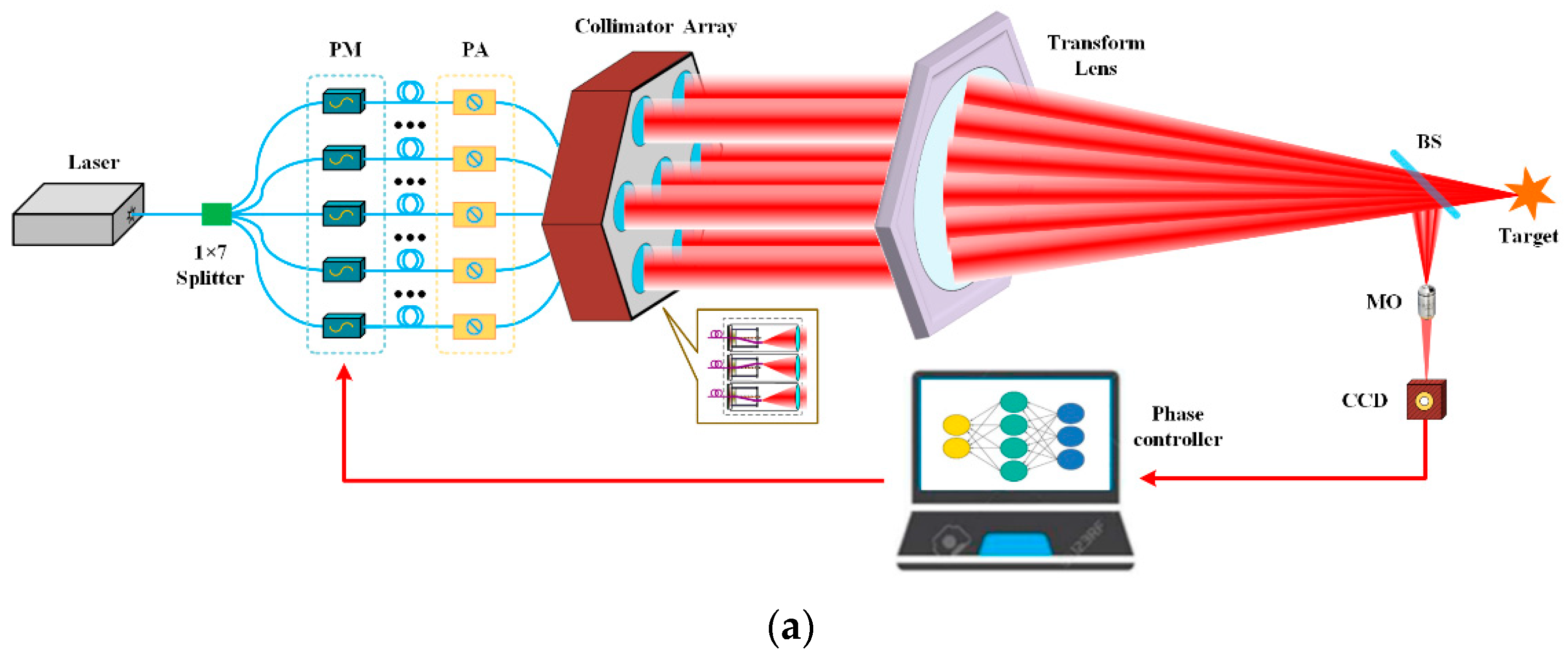
2. Principle
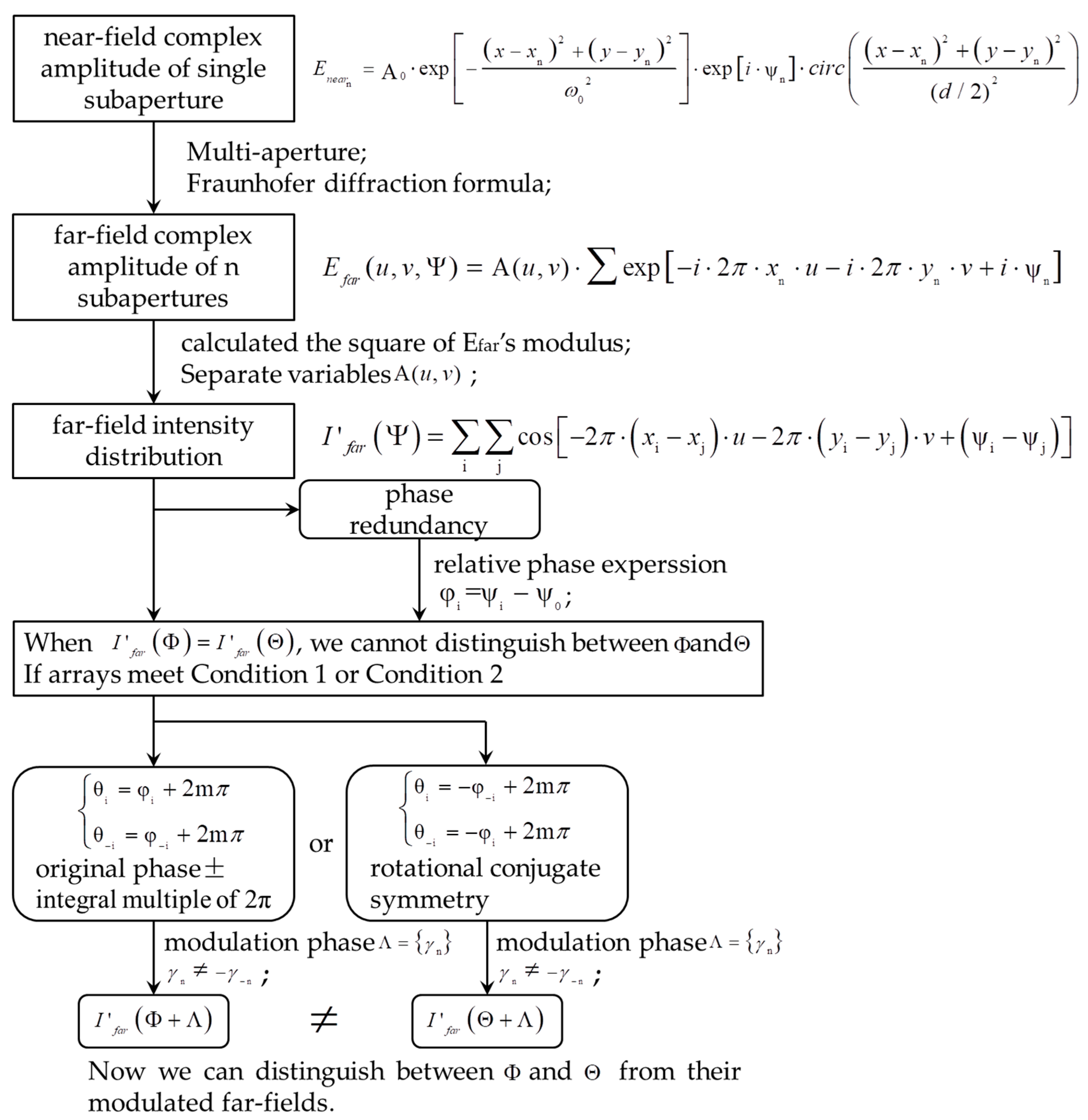
2.1. Discussion on Piston-Type Phase Ambiguity
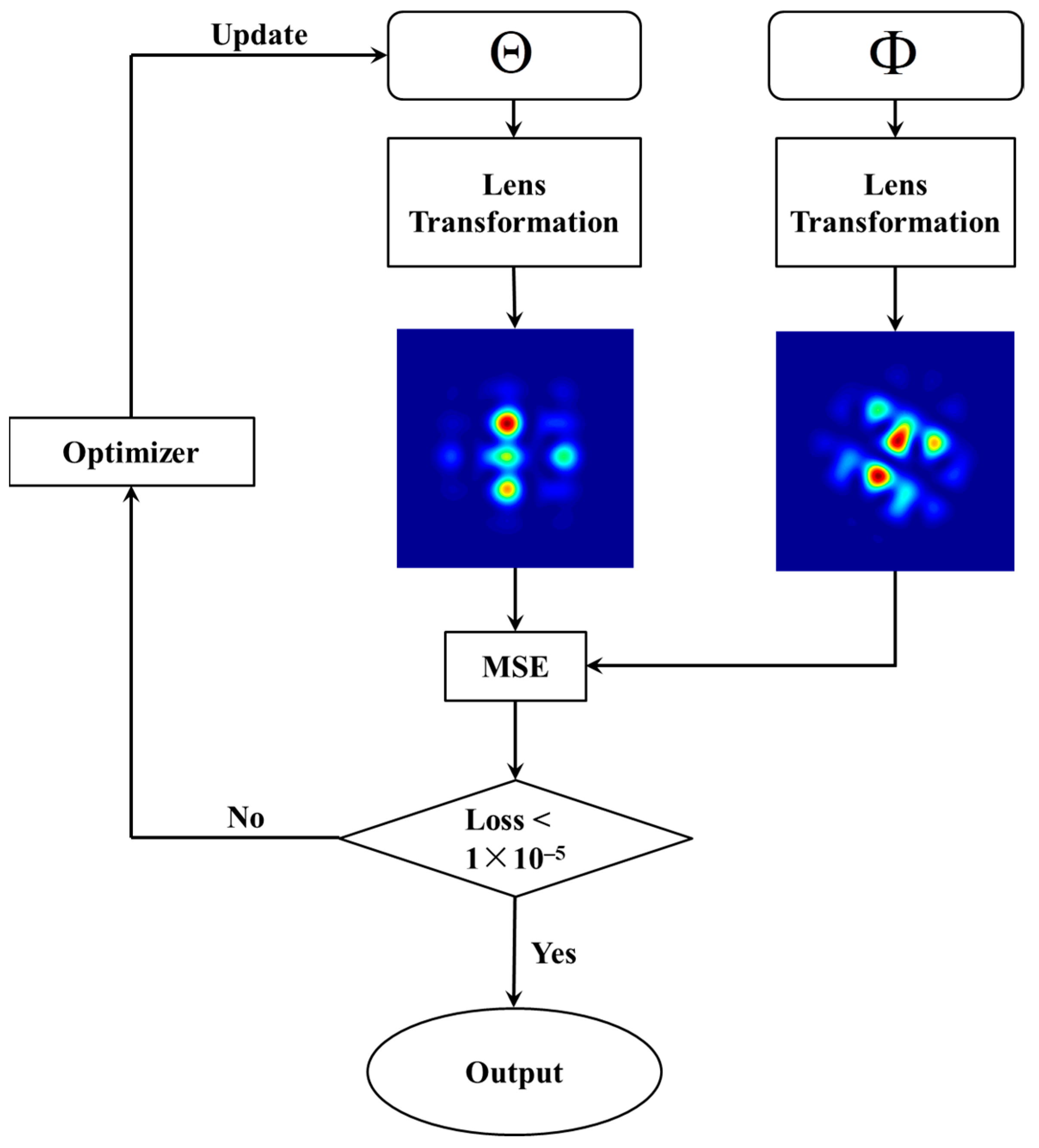
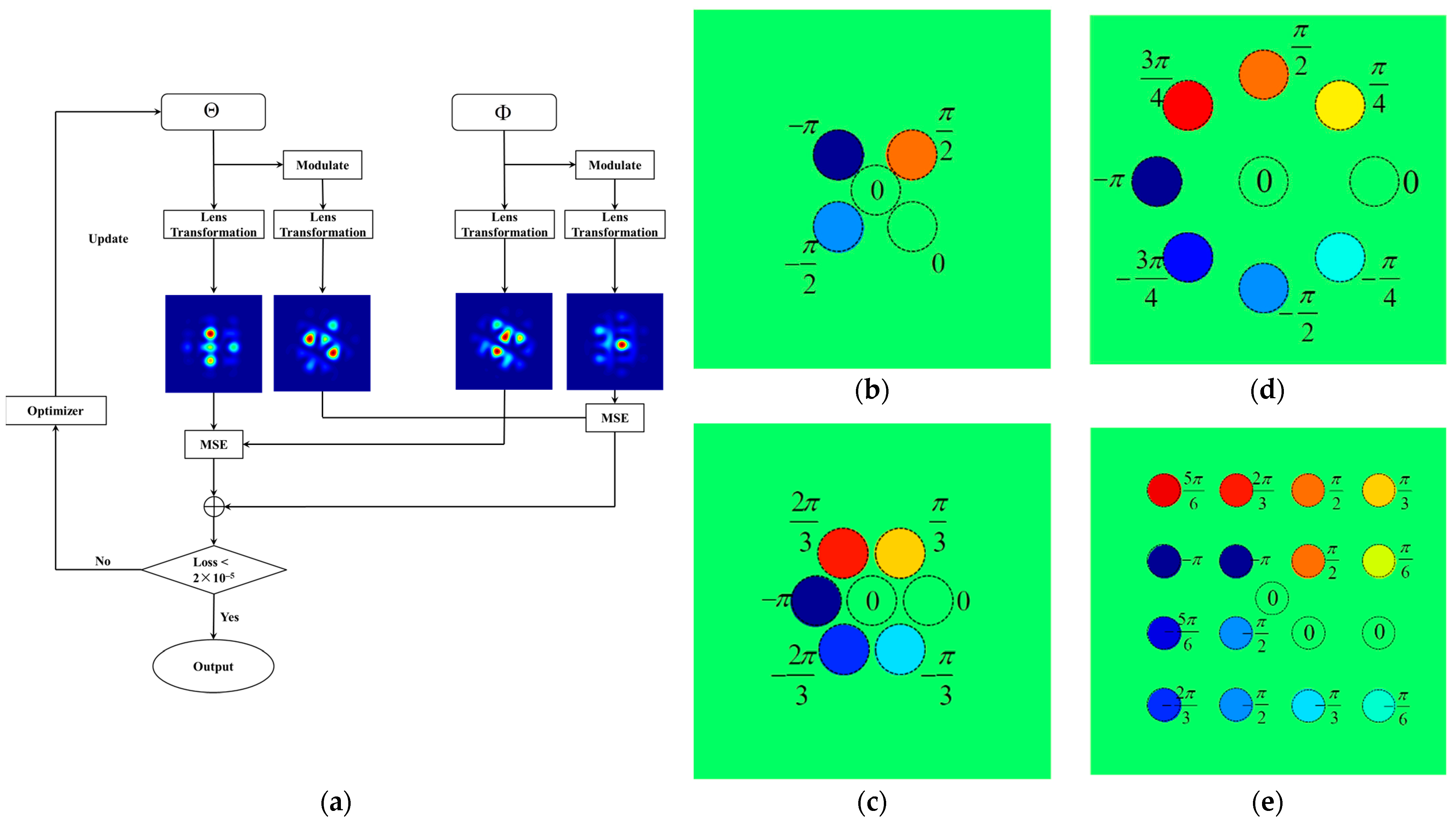
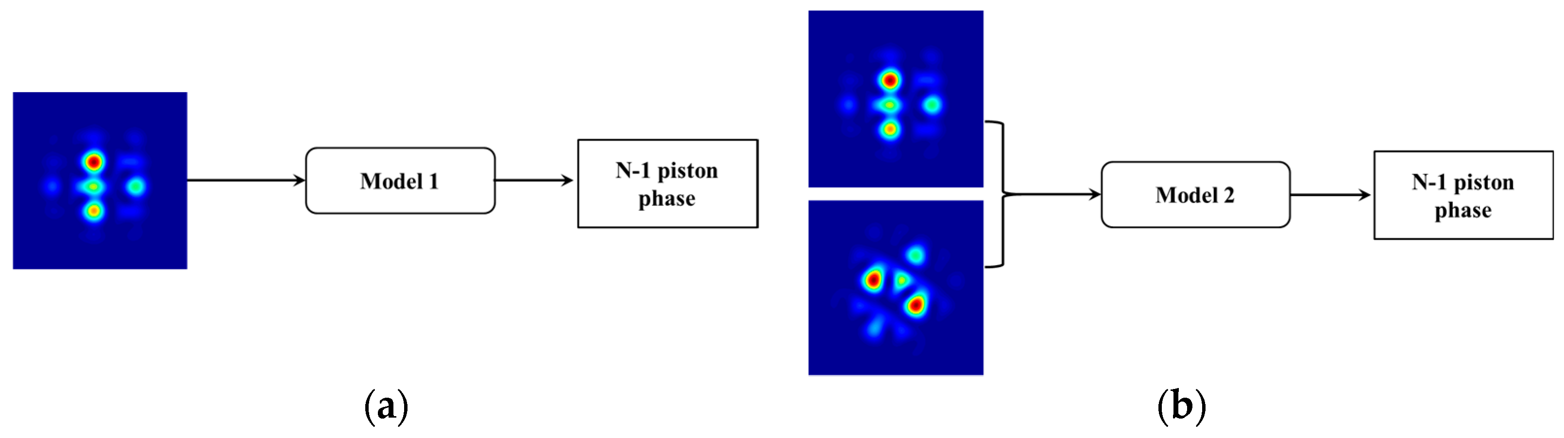
2.2. Solution to Piston-Type Phase Ambiguity
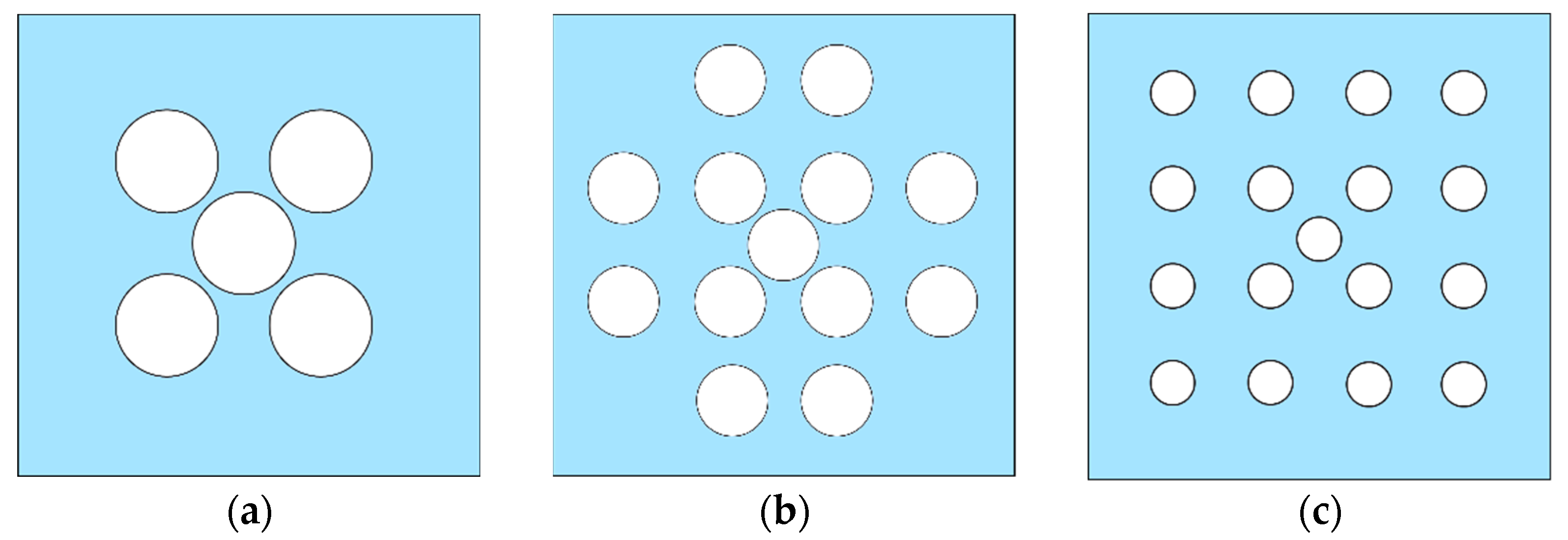
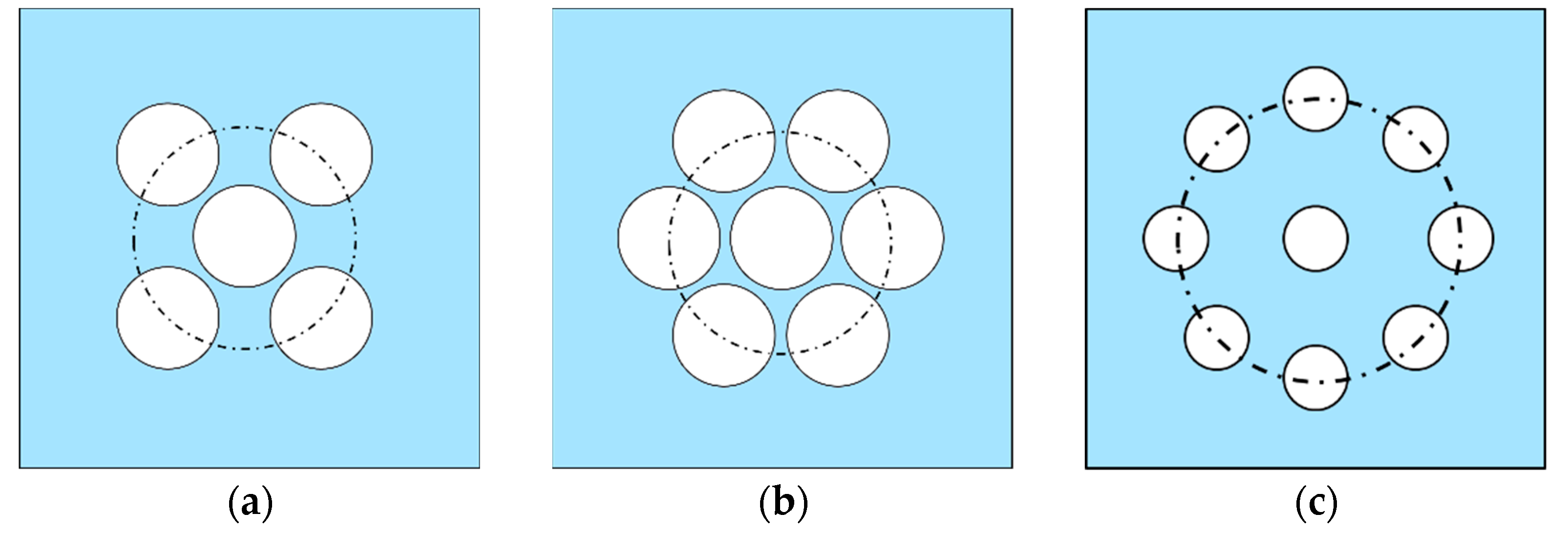
2.3. Discussion on Scalability
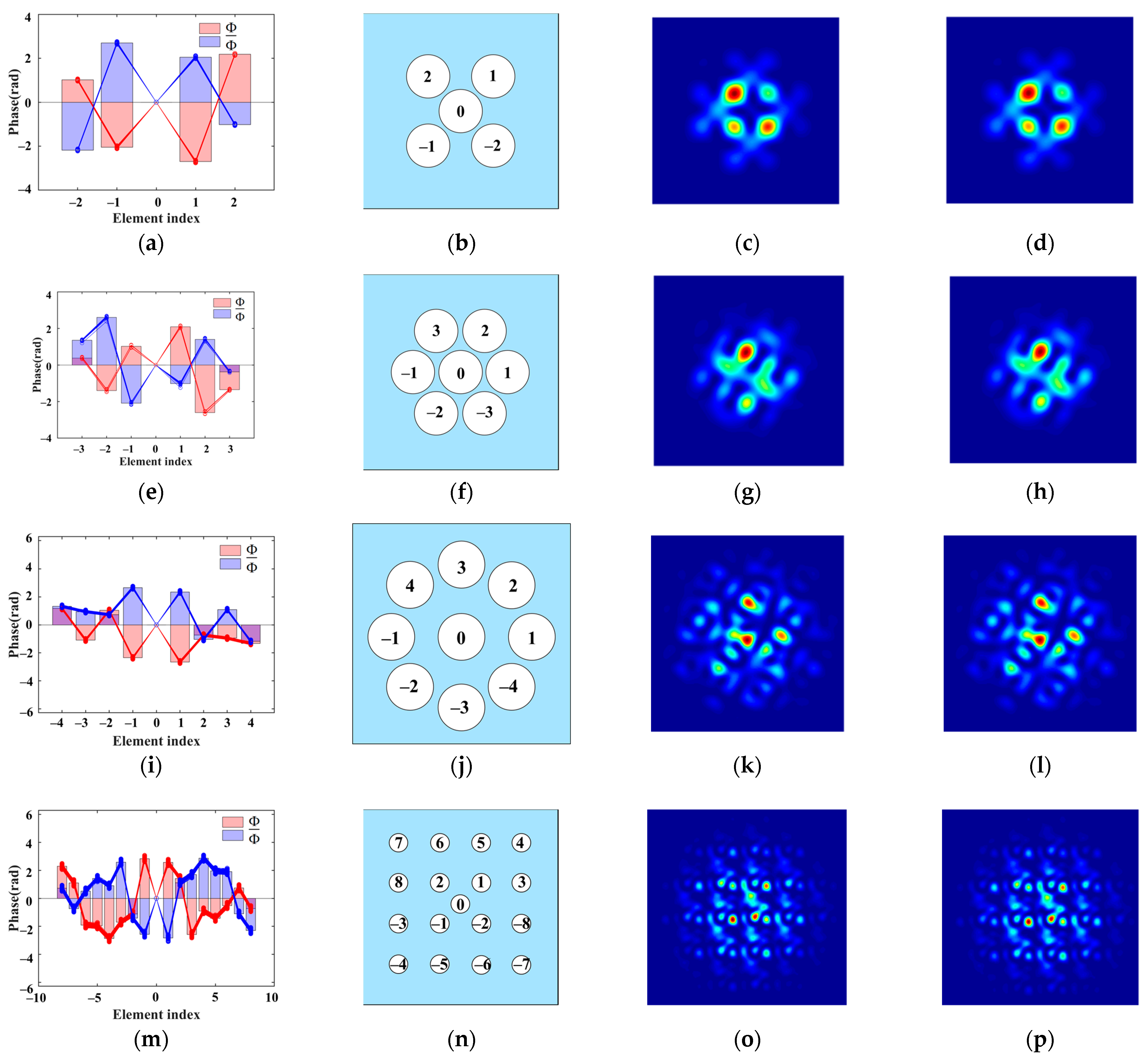
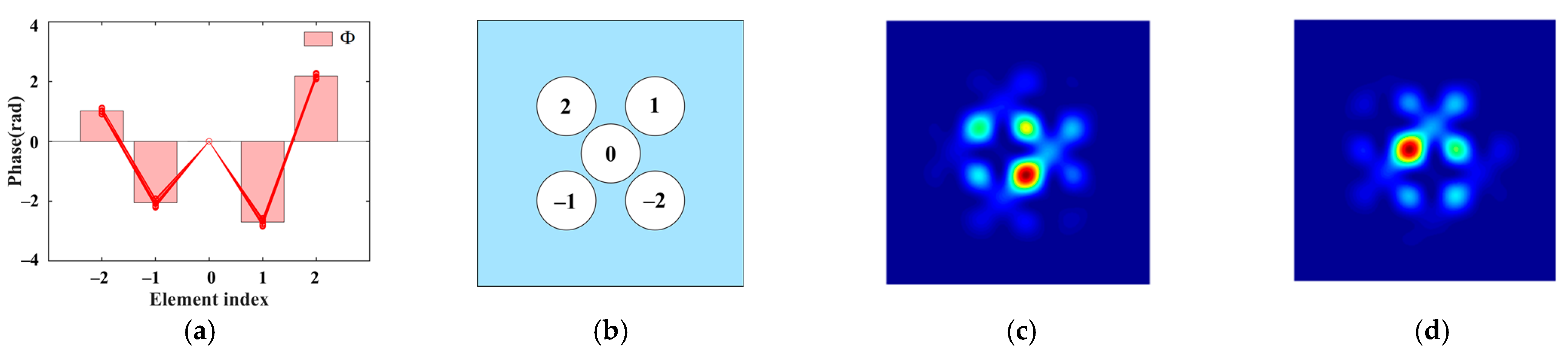
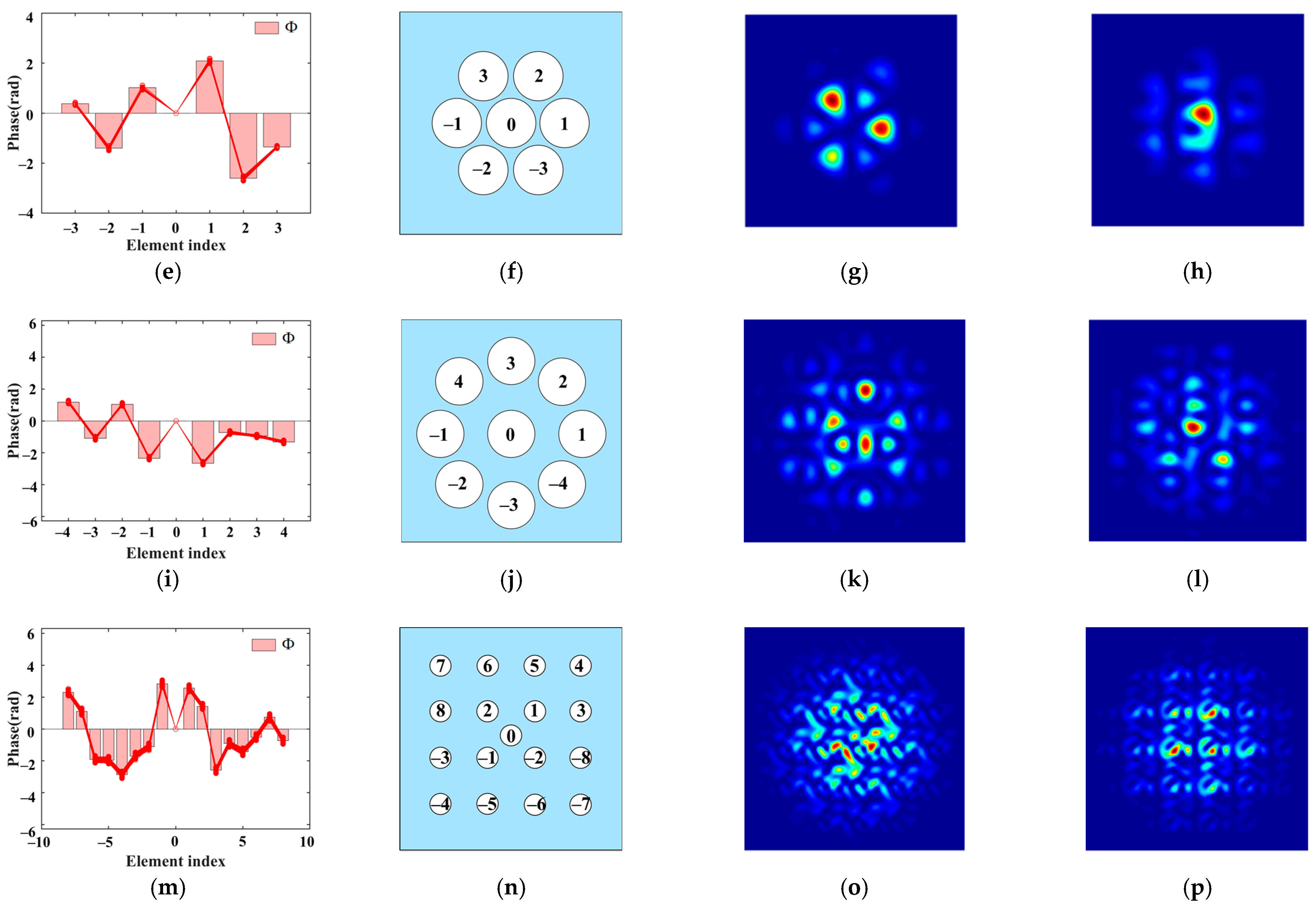
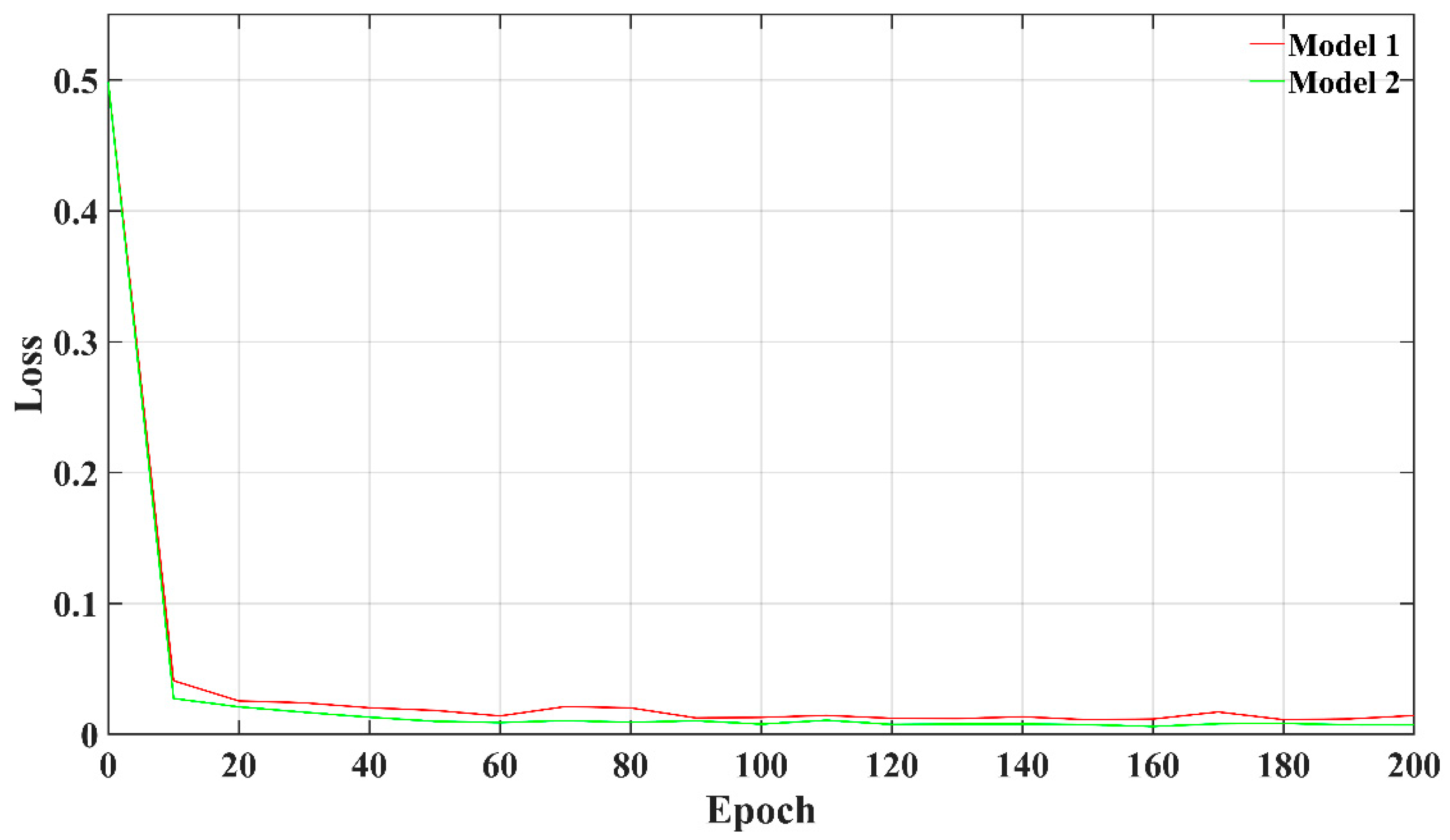
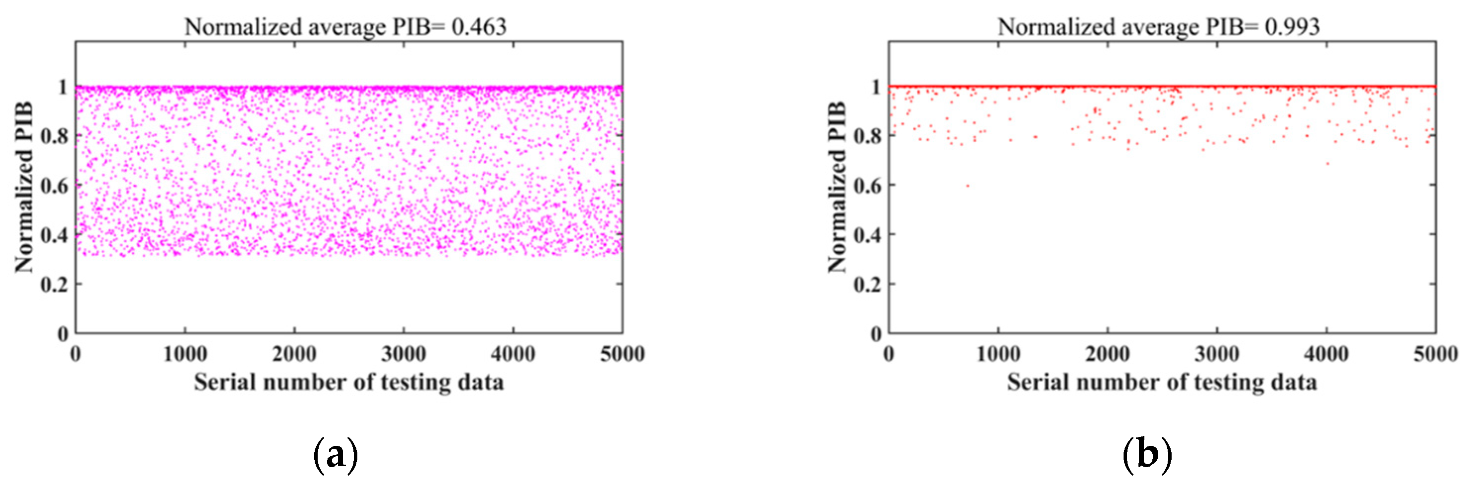
3. Simulation and Result Analysis
4. Impact of Piston-Type Phase Ambiguity
5. Conclusions
Supplementary Materials
Author Contributions
Funding
Data Availability Statement
Conflicts of Interest
Appendix A
Appendix B
Appendix C


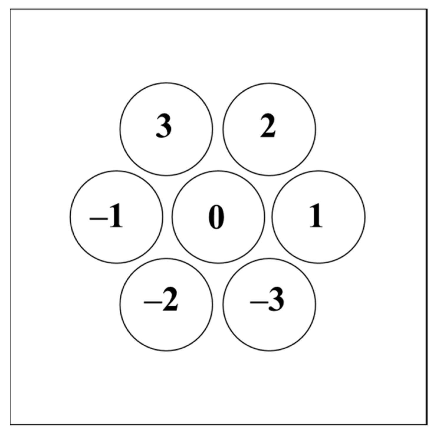
| Element Index | |||||||
|---|---|---|---|---|---|---|---|
| −3 | −2 | −1 | 0 | 1 | 2 | 3 | |
| Coordinate representation (xi, yi) | ) | ) | (−2l, 0) | (0, 0) | (2l, 0) | ) | ) |
| Components with Different Frequency | ||
|---|---|---|
| cos (−2π(4l)u) | 2cos () | 2cos () |
| sin (−2π(4l)u) | −2sin () | −2sin () |
| cos (−2π(2l)u − 2π(2l)v) | 2cos () | 2cos () |
| sin (−2π(2l)u − 2π(2l)v) | −2sin () | −2sin () |
| cos (−2π(−2l)u − 2π(2l)v) | 2cos () | 2cos () |
| sin (−2π(−2l)u − 2π(2l)v) | −2sin () | −2sin () |
| cos (−2π(3l)u − 2π(l)v) | cos ()+ cos () | cos () + cos () |
| sin (−2π(3l)u − 2π(l)v) | sin () − sin () | sin () − sin () |
| cos (−2π(2l)v) | cos () + cos () | cos () + cos () |
| sin (−2π(2l)v) | sin () − sin () | sin () − sin () |
| cos (−2π(−3l)u − 2π(l)v) | cos () + cos () | cos () + cos () |
| sin (−2π(−3l)u − 2π(l)v) | sin () − sin () | sin () − sin () |
| cos (−2π(2l)u) | cos () + cos () + cos () + cos () | cos () + cos () + cos () + cos () |
| sin (−2π(2l)u) | sin () − sin () + sin () − sin () | sin () − sin () + sin () − sin () |
| cos (−2π(l)u − 2π(l)v) | cos () + cos () + cos () + cos () | cos () + cos () + cos () + cos () |
| sin (−2π(l)u − 2π(l)v) | sin () − sin () + sin () − sin () | sin () − sin () + sin () − sin () |
| cos (−2π(−l)u − 2π(l)v) | cos () + cos () + cos () + cos () | cos () + cos () + cos () + cos () |
| sin (−2π(−l)u − 2π(l)v) | sin () − sin () + sin () − sin () | sin () − sin () + sin () − sin () |
| 1 | 7 | 7 |
Appendix D
Appendix E

References
- Fan, T.Y. Laser beam combining for high-power, high-radiance sources. IEEE J. Sel. Top. Quantum Electron. 2005, 11, 567–577. [Google Scholar] [CrossRef]
- Peng, C.; Liang, X.; Liu, R.; Li, W.; Li, R. High-precision active synchronization control of high-power, tiled-aperture coherent beam combining. Opt. Lett. 2017, 42, 3960–3963. [Google Scholar] [CrossRef]
- Vorontsov, M.; Filimonov, G.; Ovchinnikov, V.; Polnau, E.; Lachinova, S.; Weyrauch, T.; Mangano, J. Comparative efficiency analysis of fiberarray and conventional beam director systems in volume turbulence. Appl. Opt. 2016, 55, 4170–4185. [Google Scholar] [CrossRef] [PubMed]
- Cheng, X.; Wang, J.L.; Liu, C.H.; Wang, L.; Lin, X.D. Fiber Positioner Based on Flexible Hinges Amplification Mechanism. J. Korean Phys. Soc. 2019, 75, 45–53. [Google Scholar] [CrossRef]
- Chen, J.; Wang, T.; Zhang, X.; Sun, Z.; Jiang, Z.; Yao, H.; Chen, P.; Zhao, Y.; Jiang, H. Free-space transmission system in a tunable simulated atmospheric turbulence channel using a high-repetition-rate broadband fiber laser. Appl. Opt. 2019, 58, 2635–2640. [Google Scholar] [CrossRef]
- Geng, C.; Li, F.; Zuo, J.; Liu, J.; Yang, X.; Yu, T.; Jiang, J.; Li, X. Fiber laser transceiving and wavefront aberration mitigation with adaptive distributed aperture array for free-space optical communications. Opt. Lett. 2020, 45, 1906–1909. [Google Scholar] [CrossRef] [PubMed]
- Liu, R.; Peng, C.; Wu, W.; Liang, X.; Li, R. Coherent beam combination of multiple beams based on near-field angle modulation. Opt. Express 2018, 26, 2045–2053. [Google Scholar] [CrossRef]
- Weyrauch, T.; Vorontsov, M.; Mangano, J.; Ovchinnikov, V.; Bricker, D.; Polnau, E.; Rostov, A. Deep turbulence effects mitigation with coherent combining of 21 laser beams over 7 km. Opt. Lett. 2016, 41, 840–843. [Google Scholar] [CrossRef]
- Su, R.; Ma, Y.; Xi, J. High-efficiency coherent synthesis of 60-channel large array element fiber laser. Infrared Laser. Eng. 2019, 48, 331. [Google Scholar]
- Adamov, E.V.; Aksenov, V.P.; Atuchin, V.V.; Dudorov, V.V.; Kolosov, V.V.; Levitsky, M.E. Laser beam shaping based on amplitude-phase control of a fiber laser array. OSA Contin. 2021, 4, 182–192. [Google Scholar] [CrossRef]
- Chang, H.; Chang, Q.; Xi, J.; Hou, T.; Su, R.; Ma, P.; Wu, J.; Li, C.; Jiang, M.; Ma, Y.; et al. First experimental demonstration of coherent beam combining of more than 100 beams. Photon. Res. 2020, 8, 1943. [Google Scholar] [CrossRef]
- Shekel, E.; Vidne, Y.; Urbach, B. 16kW single mode CW laser with dynamic beam for material processing. Fiber Lasers XVII Technol. Syst. Int. Soc. Opt. Photonics 2020, 11260, 1126021. [Google Scholar] [CrossRef]
- Prieto, C.; Vaamonde, E.; Diego-Vallejo, D.; Jimenez, J.; Urbach, B.; Vidne, Y.; Shekel, E. Dynamic laser beam shaping for laser aluminium welding in e-mobility applications. Procedia CIRP 2020, 94, 596–600. [Google Scholar] [CrossRef]
- Zhi, D.; Ma, Y.; Tao, R.; Zhou, P.; Wang, X.; Chen, Z.; Si, L. Highly efficient coherent conformal projection system based on adaptive fiber optics collimator array. Sci. Rep. 2019, 9, 2783. [Google Scholar] [CrossRef] [PubMed]
- Mailloux, R.J. Phased Array Antenna Handbook; Artech House: Norwood, MA, USA, 2017. [Google Scholar]
- Li, F.; Geng, C.; Huang, G.; Yang, Y.; Li, X. Wavefront sensing based on fiber coupling in adaptive fiber optics collimator array. Opt. Express 2019, 27, 8943–8957. [Google Scholar] [CrossRef] [PubMed]
- Vorontsov, M.A.; Kolosov, V. Target-in-the-loop beam control: Basic considerations for analysis and wave-front sensing. JOSA A 2005, 22, 126–141. [Google Scholar] [CrossRef]
- Sun, J.; Hosseini, E.S.; Yaacobi, A.; Cole, D.; Leake, G.; Coolbaugh, D.; Watts, M.R. Two-dimensional apodized silicon photonic phased arrays. Opt. Lett. 2014, 39, 367–370. [Google Scholar] [CrossRef]
- Stamnes, J.J. Waves in Focal Regions: Propagation, Diffraction and Focusing of Light, Sound and Water Waves; Routledge: London, UK, 2017. [Google Scholar]
- Shay, T.M.; Benham, V.; Baker, J.T.; Sanchez, A.D.; Pilkington, D.; Lu, C.A. Self-Synchronous and Self-Referenced Coherent Beam Combination for Large Optical Arrays. IEEE J. Sel. Top. Quantum Electron. 2007, 13, 480–486. [Google Scholar] [CrossRef]
- Ma, Y.; Wang, X.; Leng, J.; Xiao, H.; Dong, X.; Zhu, J.; Du, W.; Zhou, P.; Xu, X.; Si, L.; et al. Coherent beam combination of 108 kW fiber amplifier array using single frequency dithering technique. Opt. Lett. 2011, 36, 951–953. [Google Scholar] [CrossRef]
- Müller, M.; Aleshire, C.; Stark, H.; Buldt, J.; Steinkopff, A.; Klenke, A.; Tünnermann, A.; Limpert, J. 10.4 kW coherently-combined ultrafast fiber laser. Opt. Lett. 2020, 45, 3083–3086. [Google Scholar] [CrossRef] [PubMed]
- Chosrowjan, H.; Furuse, H.; Fujita, M.; Izawa, Y.; Kawanaka, J.; Miyanaga, N.; Hamamoto, K.; Yamada, T. Interferometric phase shift compensation technique for high-power, tiled-aperture coherent beam combination. Opt. Lett. 2013, 38, 1277–1279. [Google Scholar] [CrossRef]
- Fsaifes, I.; Daniault, L.; Bellanger, S.; Veinhard, M.; Bourderionnet, J.; Larat, C.; Lallier, E.; Durand, E.; Brignon, A.; Chanteloup, J.C. Coherent beam combining of 61 femtosecond fiber amplifiers. Opt. Express 2020, 28, 20152. [Google Scholar] [CrossRef] [PubMed]
- Vorontsov, M.A.; Sivokon, V.P. Stochastic parallel-gradient-descent technique for high-resolution wave-front phase-distortion correction. J. Opt. Soc. Am. A 1998, 15, 2745–2758. [Google Scholar] [CrossRef]
- Geng, C.; Luo, W.; Tan, Y.; Liu, H.; Mu, J.; Li, X. Experimental demonstration of using divergence cost-function in SPGD algorithm for coherent beam combining with tip/tilt control. Opt. Express 2013, 21, 25045–25055. [Google Scholar] [CrossRef] [PubMed]
- Hou, T.; An, Y.; Chang, Q.; Ma, P.; Li, J.; Huang, L.; Zhi, D.; Wu, J.; Su, R.; Ma, Y.; et al. Deep-learning-assisted, two-stage phase control method for high-power mode-programmable orbital angular momentum beam generation. Photon. Res. 2020, 8, 715. [Google Scholar] [CrossRef]
- Liu, R.; Peng, C.; Liang, X.; Li, R. Coherent beam combination far-field measuring method based on amplitude modulation and deep learning. Chin. Opt. Lett. 2020, 18, 041402. [Google Scholar] [CrossRef]
- Tünnermann, H.; Shirakawa, A. Deep reinforcement learning for tiled aperture beam combining in a simulated environment. J. Phys. Photonics 2021, 3, 015004. [Google Scholar] [CrossRef]
- Shpakovych, M.; Maulion, G.; Kermene, V.; Boju, A.; Armand, P.; Desfarges-Berthelemot, A.; Barthélemy, A. Experimental phase control of a 100 laser beam array with quasi-reinforcement learning of a neural network in an error reduction loop. Opt. Express 2021, 29, 12307–12318. [Google Scholar] [CrossRef]
- Harvey, J.E.; Rockwell, R.A. Performance Characteristics of Phased Array And Thinned Aperture Optical Telescopes. Opt. Eng. 1988, 27, 279762. [Google Scholar] [CrossRef]
- Baron, F.; Cassaing, F.; Blanc, A.; Laubier, D. Cophasing a wide field multi-aperture array by phase-diversity: Influence of aperture redundancy and dilution. Astron. Telesc. Instrum. 2003, 4852, 663–673. [Google Scholar] [CrossRef]
- Zhang, D.; Zhang, F.; Pan, S. Grating-lobe-suppressed optical phased array with optimized element distribution. Opt. Commun. 2018, 419, 47–52. [Google Scholar] [CrossRef]
- Lei, J.; Yang, J.; Chen, X.; Zhang, Z.; Fu, G.; Hao, Y. Experimental demonstration of conformal phased array antenna via transformation optics. Sci. Rep. 2018, 8, 3807. [Google Scholar] [CrossRef] [Green Version]
- Wang, H.; He, B.; Yang, Y.; Zhou, J.; Zhang, X.; Liang, Y.; Sun, Z.; Song, Y.; Wang, Y.; Zhang, Z. Beam quality improvement of coherent beam combining by gradient power distribution hexagonal tiled-aperture large laser array. Opt. Eng. 2019, 58, 066105. [Google Scholar] [CrossRef]
- Zhi, D.; Zhang, Z.; Ma, Y.; Wang, X.; Chen, Z.; Wu, W.; Zhou, P.; Si, L. Realization of large energy proportion in the central lobe by coherent beam combination based on conformal projection system. Sci. Rep. 2017, 7, 2199. [Google Scholar] [CrossRef] [PubMed]
- Zuo, J.; Li, F.; Geng, C.; Zou, F.; Jiang, J.; Liu, J.; Yang, X.; Yu, T.; Huang, G.; Fan, Z. Experimental Demonstration of Central-Lobe Energy Enhancement Based on Amplitude Modulation of Beamlets in 19 Elements Fiber Laser Phased Array. IEEE Photonics J. 2021, 13, 1500113. [Google Scholar] [CrossRef]
- Dolph, C.L. A Current Distribution for Broadside Arrays Which Optimizes the Relationship between Beam Width and Side-Lobe Level. Proc. IRE 1946, 34, 335–348. [Google Scholar] [CrossRef]
- Goodman, J.W. Introduction to Fourier Optics; McGraw-Hill: New York, NY, USA, 2003; ISBN 978-0071142571. [Google Scholar]
- Kingma, D.P.; Ba, J. Adam: A Method for Stochastic Optimization. arXiv, 2015; arXiv:1412.6980. [Google Scholar]


Publisher’s Note: MDPI stays neutral with regard to jurisdictional claims in published maps and institutional affiliations. |
© 2022 by the authors. Licensee MDPI, Basel, Switzerland. This article is an open access article distributed under the terms and conditions of the Creative Commons Attribution (CC BY) license (https://creativecommons.org/licenses/by/4.0/).
Share and Cite
Jia, H.; Zuo, J.; Bao, Q.; Geng, C.; Luo, Y.; Tang, A.; Jiang, J.; Li, F.; Ren, J.; Li, X. Discussion on Piston-Type Phase Ambiguity in a Coherent Beam Combining System. Photonics 2022, 9, 49. https://doi.org/10.3390/photonics9010049
Jia H, Zuo J, Bao Q, Geng C, Luo Y, Tang A, Jiang J, Li F, Ren J, Li X. Discussion on Piston-Type Phase Ambiguity in a Coherent Beam Combining System. Photonics. 2022; 9(1):49. https://doi.org/10.3390/photonics9010049
Chicago/Turabian StyleJia, Haolong, Jing Zuo, Qiliang Bao, Chao Geng, Yihan Luo, Ao Tang, Jing Jiang, Feng Li, Jianpeng Ren, and Xinyang Li. 2022. "Discussion on Piston-Type Phase Ambiguity in a Coherent Beam Combining System" Photonics 9, no. 1: 49. https://doi.org/10.3390/photonics9010049