1. Introduction
Dispersion parameter of fiber is quite important in the fiber industry. There are many methods to measure the dispersion. Most of them measure the refractive index and achieve the group velocity dispersion and third order dispersion with the derivative and second derivative of the index. The pulse delay method [
1,
2] measures the time of the light with different wavelengths to pass though the fiber to calculate the refractive index. As at each wavelength a monochromatic source is needed, the method is complex with the increase of the number of sampling point to achieve high accuracy. Phase shifting method [
3] introduces an amplitude modulation after the light source and detects the modulation phase of the light after passing through the fiber. However, when the dispersion of fiber is very large, the difference of the phase and the reference phase will also be very large. In order to detect the exact phase, the step of the wavelength should be small enough, which may be costly and cumbersome. Interference method [
4,
5] can measure small dispersion, but when the length of the sample fiber is changed, the length of the reference has to, annoyingly, be changed. Using cross-correlation frequency resolved optical gating [
6], a complex behavior of orthogonal polarization modes that is different in normal and anomalous dispersion regions of the photonic crystal fiber (PCF) can be revealed. However, this method is only suitable for PCF because it estimates PCF dispersion based on interplay between nonlinear and dispersive effects during supercontinuum generation in the PCF. Optical coherence tomography can also be used to measure the refractive index of a sample. Actually, it can even provide a precise index measurement of biological tissue [
7]. However, due to the short coherence length of OCT light source, the sample cannot be too large. This is also a problem with conventional OCT dispersion measurements. Method of fingerprint-spectral wavelength-to-time mapping can measure the dispersion with high accuracy, but it employs mode-locked fiber laser as the light source, which is costly [
8], and has a fiber length limit of 0.5–100 km. Another method using transfer function [
9] is developed to indirectly measure only the third order dispersion via a sequence of iterations and needs a double-sideband suppressed carrier, variable optical delay line, optical spectrum processor and network analyzer to measure the dispersion, which is quite cumbersome, high-cost and time-consuming. While in many cases, what is really concerned is the general dispersion properties of media such as long-distance optical fibers over a wide wavelength range.
Up until now, there has been a lack of technique enabling fast and simple measurement of both the group velocity dispersion and third order dispersion of large dynamic range with high precision by utilizing a single cheap light source.
In this letter, we propose a novel technique to obtain all the dispersion parameters with no need for an ultra-wideband laser or mode-locked fiber laser. Also, by using optical computing optical coherence tomography (OC-OCT or OC
2T) [
10], we do not need any derivative operation and many index measurements. In this method, the fiber under test (FUT) is not placed in the interferometer and therefore its length has no theoretical limit. As a result, our method has large range of measurement. Therefore, we develop a new method based on OC
2T to measure dispersion for the first time. Our method provides a low-cost and simple dispersion measurement method with relatively high accuracy.
Unlike conventional OCT, OC
2T utilizes the dispersion as the method to implement optical computing to get the imaging signal and restrain the conjugate signal as well [
11]. Therefore, the dispersion and the signal have an intrinsic relationship in OC
2T. This implies a new feasibility to measure the dispersion based on OCT signal. Later, we will firstly illustrate the relationship of the fiber dispersion and the signals in OC
2T and give a simple way to measure the dispersion.
2. Methods
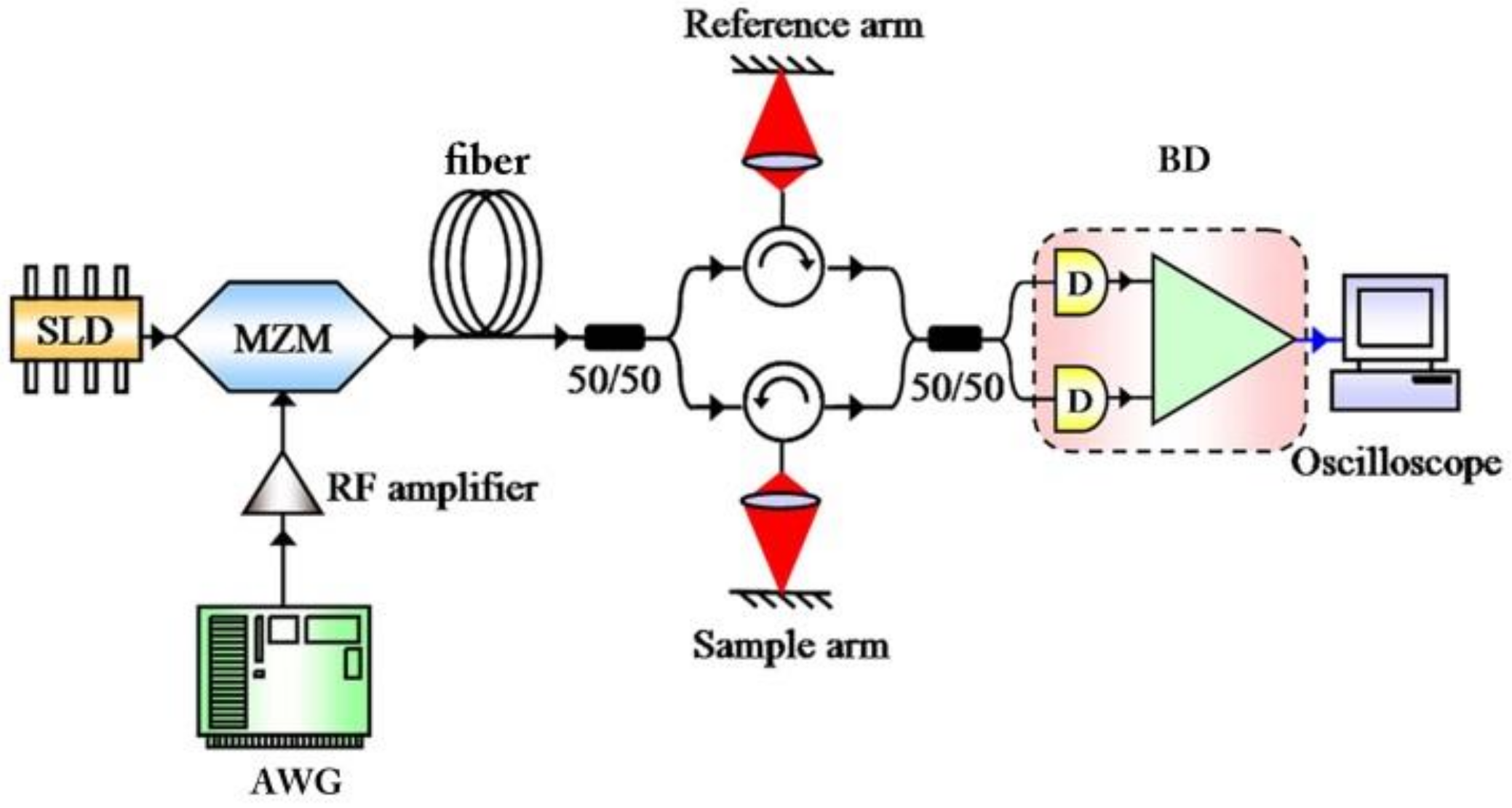
The optical design of the OC
2T is shown in
Figure 1. In the experiment, we use an LED as the light source with a center wavelength of 1550 nm and FWHM of 40 nm. The bandwidth of BD is 20 GHz. The complex amplitude of light from SLD is expressed as:
where
t is the time variable,
ω the frequency of light,
ω0 is the center frequency and
S0 is a constant. γ = (2ln2)
1/2λ
02/(cπΔλ) describes the bandwidth of the light in angular frequency and Δ
λ is the FWHM bandwidth in wavelength.
An MZM is used to modulate the light. The modulation function
m(
t) is generated by an arbitrary waveform generator (AWG). The signal after MZM is:
where
m2(
t) = [1 + cos(
at2)]/2 and
a is a constant. In the experiment, the parameter
a is 1.6 × 10
−17 s
−2.
A section of fiber is used as dispersion media after MZM. We define the optical pathlength:
where
L,
n and
ω0 are fiber length, refractive index and center frequency of light, respectively. While
n0,
βL and
βL2 are refractive index at
ω0, group-velocity dispersion and third order dispersion of the fiber, respectively.
The signal after fiber is:
T is the duration of the modulation signal
m(
t).
Therefore, the signal passes through the interference and reaches the balanced detector [
9]:
ns represents the sample refractive index, Δ
l the optical path difference,
l the length of the dispersion media and
βl the group velocity dispersion of the insert media.
rs,
rr represent the reflectivity of the sample and reference arm, and
z the distance between the imaging point and the surface of the sample.
As a mirror is used as the sample, i.e.,
z = 0, we have:
We neglect the DC background in Equation (6) and rewrite the signal of the OC
2T system as:
As shown in Equation (7), the signal appeared at
α2 = ±
β2, the first term appeared at
α2 =
β2 may be defined as the signal, and thus the second term appeared at
α2 = −
β2 as its conjugate. As
α2 is in direct proportion to the group-velocity dispersion, the value of group dispersion will be reflected in the position of the signal. Hence:
Based on Equation (8), the signal position
t′ is proportional to Δ
l, and the scale factor is associated with the group-velocity dispersion of the fiber. Therefore, we can calculate the group-velocity dispersion by measure the relationship between Δ
l and
t′:
Now we consider the axial resolution of the signals. Because there is no dispersion difference between the sample arm and reference arm, we have
β3 = 0 and the resolution is affected by
α3. As the value of
α3 is a function of the third order dispersion
βl2 and the position of the signal
t′, the signal at different
t′ will have different resolution, and the change of resolution is determined by
βl2. As both signals are Gaussian shape, the axial resolution of the signal and its conjugate are their FWHMs:
where δ
z0′ = (2ln2)
λ02/(πΔ
λ) is exactly the axial resolution of traditional OCT
Based on Equation (10), the resolution of OC
2T changes with
α3 and
α3 is a variable of
t′ and third order dispersion
βL2. To measure the resolution, we can calculate the third order dispersion of the fiber.
Although we can only calculate the absolute value of α3 from Equation (11), the sign is easy to determine, because α3 linearly changes with t′ and is always positive at t′ = 0. Therefore, we can calculate the third order dispersion by Equation (11).
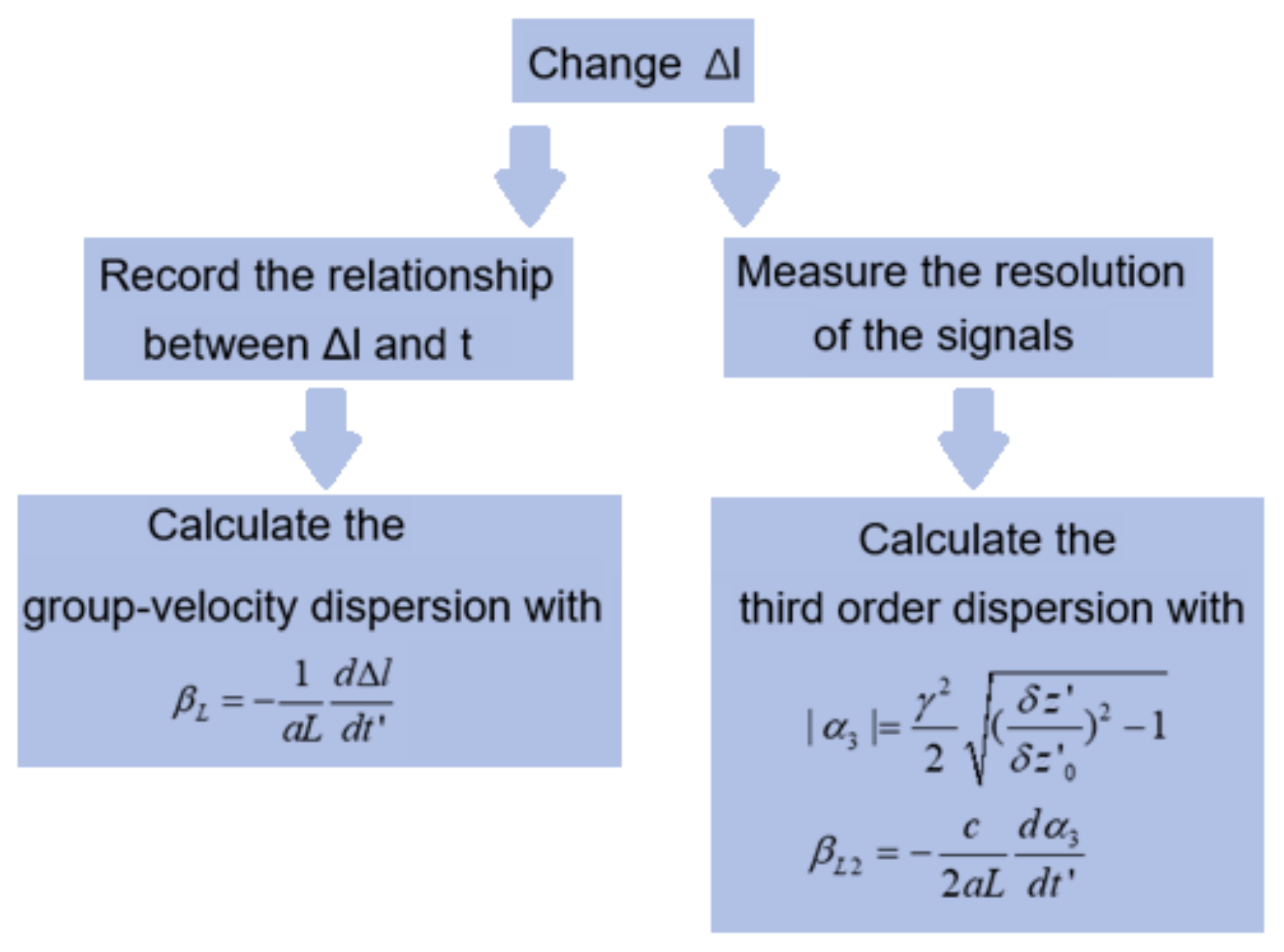
The flow chart is shown in
Figure 2. The fiber under test is placed after MZM. We then change the optical path difference between the reference arm and sample arm Δ
l and record the signal position
t′ and resolution
δz′. Finally, we can calculate the group-velocity dispersion and third order dispersion by Equations (8) and (11).
3. Experiments Result
We measure the dispersion parameter of 10 km of single mode fiber (SMF, βL = 6.5 × 10⁻¹⁸ s, βL2 = 2.2 × 10⁻³² s2) to prove the ability of our method.
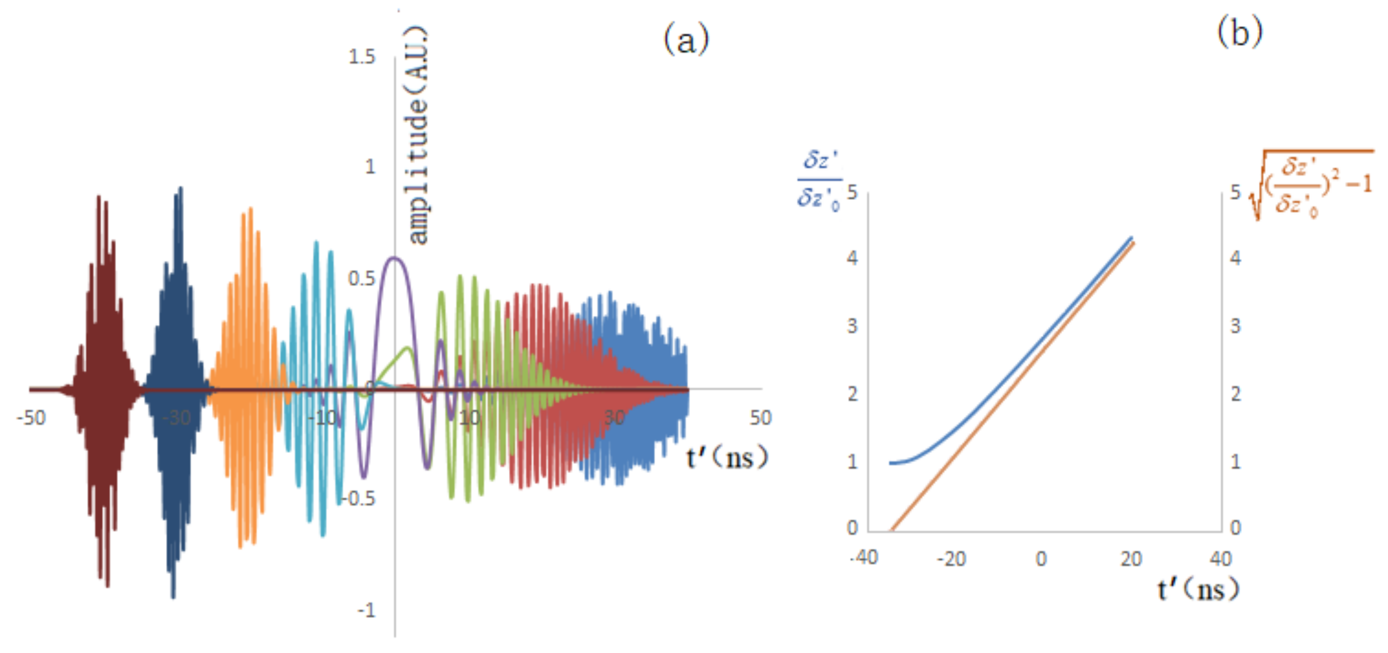
In order to verify the experiment result, we first use the same parameters of our experiment to do the simulation, as shown in
Figure 3. We measure the broadening of the simulation signals and find that [(
δz′/
δz0′)
2−1]
1/2 is linear with
t′, which is consistent with the theory.
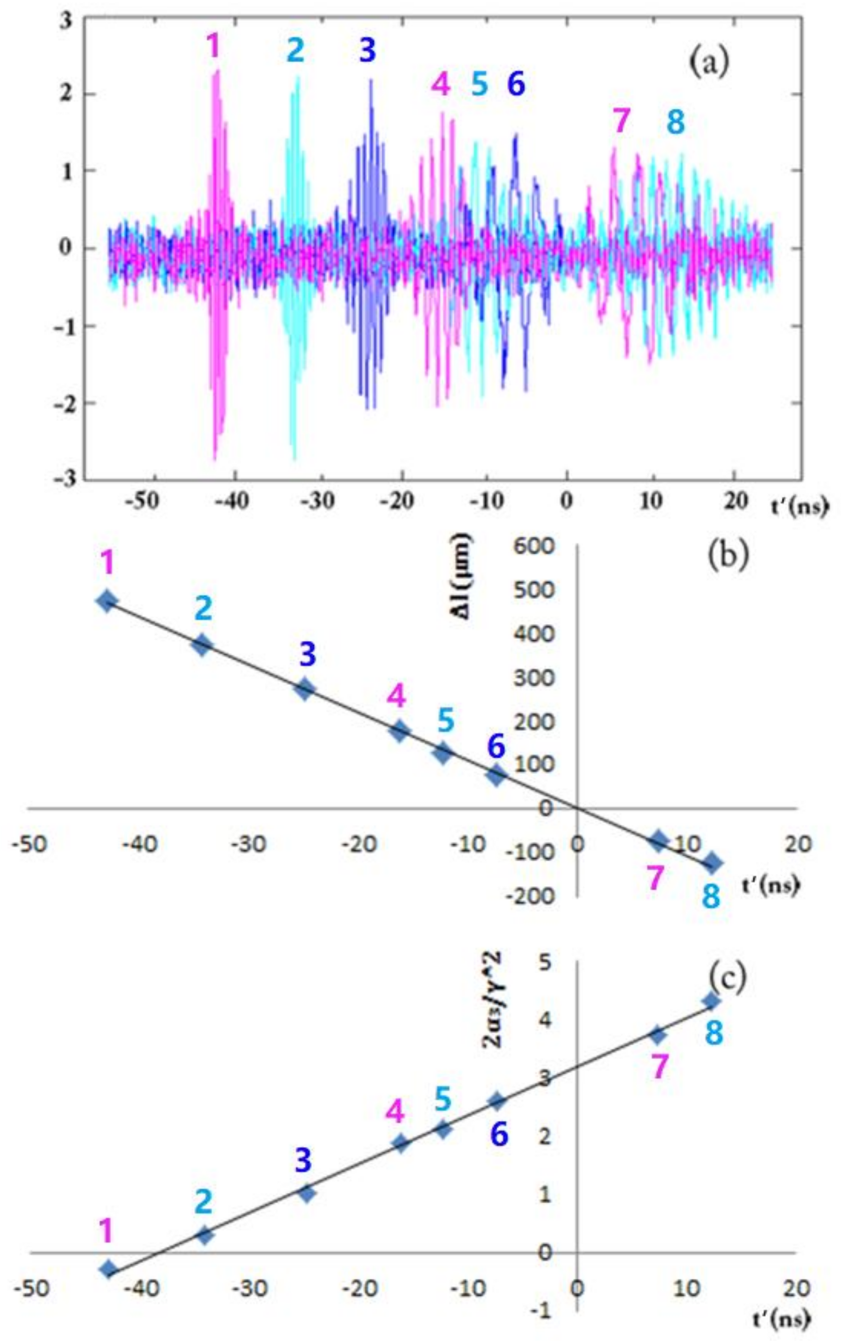
Figure 4 shows the experiment result, where we measured the signal at different
t′ by changing the optical path difference Δ
l. In
Figure 4a, we can see that the position and the width of the signal are changing with the optical path difference Δ
l. In
Figure 4b,c, we prove experimentally that the optical path difference Δ
l and
α3 are linear with
t′, which is in consistent with the theoretical results. We find the relationship between Δ
l and
t′ in
Figure 4b and calculate the slope d(Δ
l)/d
t′ = −(10.9 ± 0.6) μm/ns. The group-velocity dispersion can be deduced from Equation (7):
The third order dispersion can also be calculated by measuring the resolution broadening. We measure the resolution and calculate 2|
α3|/
γ2 = [(
δz′/
δz0′)
2 − 1]
1/2, as shown in
Figure 4c. The slope 2/
γ2 ∗ d(
α3)/d
t′ = −(0.084 ± 0.004) ns
−1. Therefore, the third order dispersion can be obtained from Equation (8):
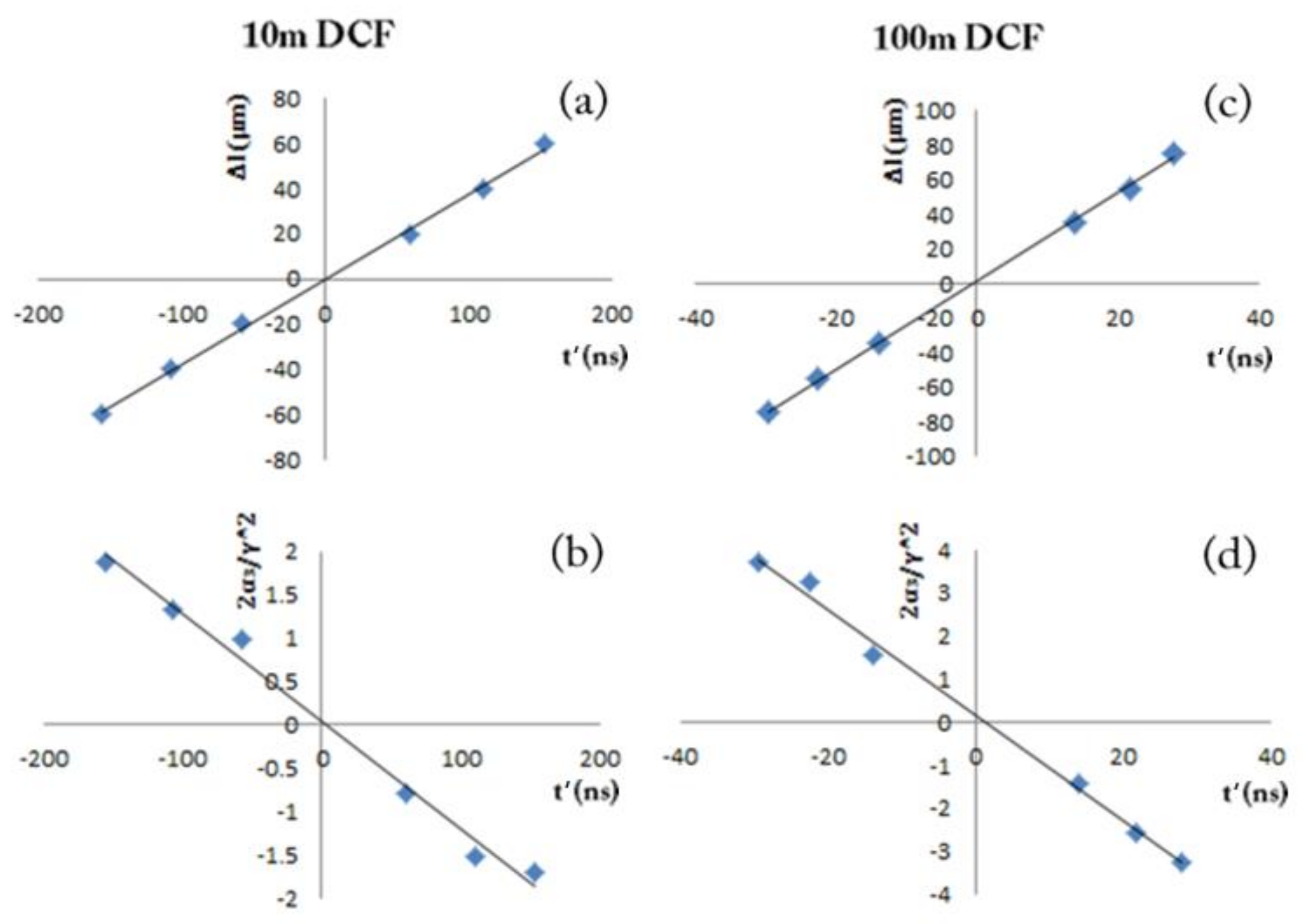
We also measure the dispersions of some dispersion compensating fibers (DCF) with different lengths (DCF-G.655/250, WuHan ChangFei,
βL = −1.4 × 10
−16 s,
βL2 = −3.2 × 10
−30 s
2) to further evaluate our method experimentally, as shown in
Figure 5. We can see that our method can measure the dispersion of short fibers even if the fiber is only 10 m long.
As our method is computationally simple, we can calculate the slope by LINEST function in Excel. The LINEST function uses the least square method.
The comparison of dispersion parameters measured with our method and the theoretical value was shown in
Table 1. In the table, the measurement results of our method are in good agreement with the factory specifications.
4. Discussion
As shown in
Table 1, both the group velocity dispersion and the third order dispersion are well in agreement with nominal value. Also, we can find that relative uncertainty is smaller if the sample has larger dispersion
βl ∗ L or
βl2 ∗
L, i.e., longer length or larger dispersion parameter.
The instrument cost and complexity of our method are far less than those of pulse delay method, but our method can achieve comparable accuracy when we measure 10,000 m SMA. Although our method has relatively large error when measuring the group-velocity dispersion of short fibers, similar to other methods such as the pulse delay method, we can still measure the third order dispersion with higher accuracy than conventional methods even if the fiber is only 10 m long.
The measurement accuracy of the group-velocity dispersion mainly depends on the uncertainty of each point to measure Δ
l and
t′. Because Δ
l is changed by a translation stage which has an accuracy of as high as 1 μm, its uncertainty can be neglected. The uncertainty of the signal position
t′ is half of the resolution. Therefore, we have:
The uncertainty of the third order dispersion mainly comes from the measurement error of resolution broadening and
t′. As the uncertainty of resolution broadening is affected by the distortion of modulation and signal detection, which is complicated to measure, we thus use the standard deviation of the slope of linear regression as an estimate. So, we have:
.
Compared with the traditional methods, our measurement system is simple and easy to set up. Also, both group velocity dispersion and the third order dispersion can be measured, and the results are well in agreement with nominal value. Our method is more compact and low-cost than conventional methods such as the pulse delay method and interference method because they employ a lot of mono-chromatic sources or reference arms with different lengths. Also, we obtain the group-velocity dispersion and the third order dispersion by calculating the slope of the signal position and resolution at different t′. Therefore, even if some measuring points have large error, the slope does not change that much. This implies that the measurement with our method is more robust and has good stability.
The comparisons between our method and some conventional methods are shown in
Table 2.
The phase shifting method has a limited dynamic range caused by the need of a single period of the phase modulation, while the interference method has its dynamic range limit around the length of the reference arm. Our method can measure the dispersion of fibers of any lengths, because the fiber under test (FUT) is not placed in the interferometer and therefore its length has no theoretical limit. However, the minimum value which is suitable for measurement is limited by the measurement accuracy. As already discussed, when measuring the group-velocity dispersion of short fibers, our method can still implement measurements, but with relatively large errors. Therefore, our method is more suitable for measuring samples with group-velocity dispersion larger than 10 m DCF. However, as for the third order dispersion, our method can obtain reliable results even if the fiber is only 10 m long.
In the following study, we will further improve the measurement accuracy and enable the method to measure even smaller dispersion. The SNR of the OC2T system will be further improved so that the position and resolution of the signal can be more precise. As a result, the standard deviation of the slope of linear regression will be smaller and the measurement accuracy can be further improved.

 ,
, 


