Article

Tensor Dictionary Learning with an Enhanced Sparsity Constraint for Sparse-View Spectral CT Reconstruction

1
State Key Laboratory for Electronic Testing Technology, North University of China, Taiyuan 030051, China
2
School of Software, Shanxi Agricultural University, Taigu District, Jinzhong 030800, China
3
Ping An Technology, U.S. Research Laboratory, Palo Alto, CA 94306, USA
*
Author to whom correspondence should be addressed.
Photonics 2022, 9(1), 35; https://doi.org/10.3390/photonics9010035
Submission received: 14 December 2021 / Revised: 31 December 2021 / Accepted: 5 January 2022 / Published: 8 January 2022
(This article belongs to the Special Issue X-ray Luminescence and Fluorescence)

Abstract

:
Spectral computed tomography (CT) can divide collected photons into multi-energy channels and gain multi-channel projections synchronously by using photon-counting detectors. However, reconstructed images usually contain severe noise due to the limited number of photons in the corresponding energy channel. Tensor dictionary learning (TDL)-based methods have achieved better performance, but usually lose image edge information and details, especially from an under-sampling dataset. To address this problem, this paper proposes a method termed TDL with an enhanced sparsity constraint for spectral CT reconstruction. The proposed algorithm inherits the superiority of TDL by exploring the correlation of spectral CT images. Moreover, the method designs a regularization using the L0-norm of the image gradient to constrain images and the difference between images and a prior image in each energy channel simultaneously, further improving the ability to preserve edge information and subtle image details. The split-Bregman algorithm has been applied to address the proposed objective minimization model. Several numerical simulations and realistic preclinical mice are studied to assess the effectiveness of the proposed algorithm. The results demonstrate that the proposed method improves the quality of spectral CT images in terms of noise elimination, edge preservation, and image detail recovery compared to the several existing better methods.

1. Introduction

Computed tomography (CT) can provide intramural organ tissue and structure information via a nondestructive imaging technology, which has been extensively employed in medical diagnosis, industrial detection, and archaeology [1,2]. However, traditional CT still cannot satisfy many practical requirements due to its limitations. First, it uses the energy integration detectors and performs poorly at identifying the energy of X-ray photon, leading to energy-dependent information missing. Second, the reconstructed images often suffer from strong beam hardening artifacts [3,4]. Moreover, it increases radiation risk because multiple scans are needed to obtain multiple energy projections [5,6]. To solve the limitations, spectral CT (also known as multi-energy CT) has attracted increasing attention because of its superiority in material decomposition, lesion detection, and tissue characterization [7,8]. Dual-energy CT (DECT) is a common and typical spectral CT that collects projections using two different X-ray spectral. However, most DECT scanners utilize energy-integrating detectors and there inevitably exists spectral overlap, which reduces the energy resolution [9]. Recently, the photon counting detector-based spectral CT has gained considerable attention; it divides the received photons into multiple energy channels and generates multi-channel projections at the same time, providing more spectral information than the DECT [10]. Nevertheless, because of the limited number of photons in the corresponding energy channel, single-channel projections are usually affected by severe quantum noise, leading to low signal-to-noise ratio (SNR) measurements [11]. Therefore, how to improve the image quality of PCD-based spectral CT has become a hot research topic.
A large number of spectral CT reconstruction algorithms have been developed to improve the quality of images from the contaminated projections. At the very beginning, some traditional methods were used for spectral CT reconstruction. In 2012, Xu et al. regarded the spectral projection data as a traditional dataset and reconstructed an image in a single energy channel independently using TV regularization [12]. Subsequently dictionary learning was utilized for the reconstruction of spectral CT [13,14,15]. Zhao et al. proposed an iterative reconstruction algorithm of spectral breast CT based on tight frames [16]. Reconstruction methods such as the above only consider the sparsity in the spatial domain and ignore the sparsity in the spectral channel domain. To link the correlation between different channels, Kim et al. the proposed low rank (LR) algorithm for spectral CT [17]. By combining TV and LR constraints, the TVLR method showed a significant improvement compared to the TV-only algorithm [18]. Rigie et al. developed an algorithm based on total nuclear variation regularization to maintain image features for spectral CT reconstruction [19]. In 2014, Semerci et al. proposed a spectral CT reconstruction algorithm combining a nuclear norm based on tensor and TV [20]. Gao et al. modeled a spectral CT image as the superposition of a low-rank and a sparse matrix, and employed a reconstruction algorithm based on a framework PRISM (prior rank, intensity, and sparsity model) [21]. Subsequently, the PRISM was improved by combining it with the higher-dimensional tensor approach [22]. Wu et al. combined a weighted adaptive TV regularization and image-spectral tensor factorization for photo-counting CT imaging [23]. To utilize the non-local similarity in the spatial domain, Wu et al. considered the correlation and non-local similarity among energy channels simultaneously, then proposed a cube matching frame based on the spatial-spectral domain [24]. Later, Hu et al. proposed an algorithm based on tensor combining the similarity with the spectral-image domain [25]. While the above methods improve the spectral CT image quality greatly, if a high-quality prior image containing the full energy spectrum is introduced, the quality of the reconstructed image will be further improved [26,27,28].
Tensor dictionary learning (TDL) is an extension of traditional vectorized dictionary learning [29]. Concretely speaking, the TDL method extracts tensor patches from the image tensor to train a tensor-based dictionary, which is used to sparsely represent image tensor patches during an iterative reconstruction process. Because TDL fully integrates sparsity in both spatial and spectral dimensions, the noise and artifacts in reconstructed images can be effectively suppressed [30]. The TDL-based method has been widely used in hyperspectral images; Peng et al. employed decomposable non-local TDL to denoise multi-spectral image [31]. Gong et al. proposed a low-rank tensor dictionary learning method for hyperspectral image denoising and achieved better denoising results [32]. Then in the CT reconstruction field, Tan et al. considered the relevance among atoms and across phases and trained a tensor spatial-temporal dictionary for dynamic CT reconstruction [33]. Zhang et al. utilized the correlation of images from different energy channels and developed TDL for spectral CT reconstruction [30]. While the TDL method improves the image quality by exploring the correlation of spectral CT images, it may decrease the ability of edge protection under the situation of sparse view and low dose [34]. Recently, the image gradient L0-norm, as an important regularization term, has been widely applied to image smoothing, image segmentation, and image restoration [35,36,37]. Subsequently, it has gained great attention in CT reconstruction, especially in reconstructing limited-view, sparse-view, and low-dose CT images, which has a better performance in maintaining image edge, reducing artifacts, and suppressing noise than the image gradient L1-norm. The main reason is that the image gradient L0-norm calculates the number of non-zero pixels instead of penalizing the large image gradient magnitudes. Therefore, it is more suitable to protect edge information.
In this work, inspired by the pioneering study of TDL, and to address the limitation of the TDL-based method for spectral CT reconstruction, this paper introduced the L0-norm of image gradient and a prior image to the TDL model to further enhance the ability to recover subtle image structures effectively. The proposed algorithm inherits the superiority of the TDL method. Moreover, the algorithm designs a regularization using the image gradient L0-norm and a prior image in each energy channel simultaneously. The regularization term not only constrains the sparsity of a single image to improve the ability to preserve edge information and reduce noise, but also introduces a prior image combining with the image gradient L0-norm to constrain the difference among images to guide the protection of subtle image details.
The main contribution of this work has three aspects. First, the L0-norm of the image gradient is introduced to the TDL-based model to improve the edge retention ability. Second, the prior image is used to enhance the detail recovery ability under the constraint of the image gradient L0-norm. Third, an efficient split-Bregman algorithm is utilized to address the objective minimization model.
The rest of this article is organized as follows. Section 2 briefly introduces related mathematical foundations and basic theories. Section 3 presents the solution of the proposed mathematical model in this paper. In Section 4, numerical simulation and preclinical mouse dataset experiments are carried out. Finally, we present a conclusion and discussion in the last section.

2. Fundamental Theory Methods

2.1. Tensor Dictionary Learning

A tensor is a multi-dimensional data array. An N-order tensor is written as χ I 1 × I 2 × × I k × × I N , where Ik is the length of the kth dimension (k = 1, 2, …N). Elements of χ are denoted as x i 1 i 2 i N ( 1 i k I k , k = 1 , 2 , N ) . Especially when N = 1, tensors are vectors, and when N = 2, tensors are matrices. A tensor can multiply with a vector or a matrix. The mode-k product of a tensor χ by a matrix P J × I k is expressed as χ × k P I 1 × × I k 1 × J × × I k + 1 × × I N , whose element is calculated by i k = 1 I k x i 1 i 2 i N p j i k . In this work, we only consider a third-order tensor, and suppose χ ( n ) N 1 × N 2 × N 3 (n = 1, 2, …N) to be a third-order tensor. The TDL can be regarded as solving the following problems:
arg min D , α n n = 1 N | | χ ( n ) D × 4 α n | | F 2 , s . t . | | α n | | 0 L
where D = { D ( k ) } R N 1 × N 2 × N 3 × K (k = 1, 2, … K) is a tensor dictionary that could be trained by utilizing the K-CPD algorithm [38], K represents the number of atoms in the dictionary, αn is the coefficient vectors, L is the sparsity level, ||•||F and ||•||0 represent Frobenius-norm and L0-norm. Equation (1) could be addressed by using the alternating direction method of multipliers (ADMM) [39]. Firstly, the multi-linear orthogonal matching pursuit (MOMP) method is used to update sparse coefficient vectors αn while fixing the tensor dictionary D. The second step is to update the tensor dictionary D with fixed sparse coefficient vectors αn. According to the alternating update methods, the optimal D and the corresponding αn can be obtained at the same time.

2.2. TDL for Spectral CT Reconstruction

The TDL model for spectral CT reconstruction could be denoted as follows [30]:
arg min x , α j , n j 1 2 c = 1 C | | A x c p c | | 2 2 + λ 2 ( j | | Ε j ( χ ) D n × 4 n j D × 4 α j | | F 2 + j ν j | | α j | | 0 )
where χ N 1 × N 2 × C are third-order reconstructed image tensors, where N1 and N2 represent width and height of the reconstructed image, respectively; P J 1 × J 2 × C are projection data tensors, where J1 is the number of the detector and J2 is the projection views. C represents the energy channels. xc and pc are the vectorized cth image and projection, respectively, A is the system matrix, nj is the mean vector of every channel, the operator Ej is utilized to extract the jth small tensor block from χ, where the size of the tensor block is M·M·C, αj represents the sparse representation coefficient of the corresponding tensor block. D = { D ( k ) } M × M × C × K represents the trained tensor dictionary; D n = { D ( k ) } M × M × C × C denotes the mean removal process. λ is a key parameter balancing the data fidelity and the sparse representation; the parameter vj is used to balance the representation accuracy and sparse level. To avoid repetition, the solution of Equation (2) is described in the next section. Because the system matrix A depends on system geometry, a different scanning strategy will generate a different A, which will affect the values of parameter λ. To solve the problem, we rewrite λ as follows:
λ = η C i 1 = 1 N 1 i 2 = 1 N 2 [ A T A ] i 1 i 2 j c = 1 C i 1 = 1 N 1 i 2 = 1 N 2 [ E j T E j ] i 1 i 2
where η is a scale parameter, which balances the data fidelity term and a sparse representation regularization term.

2.3. L0-Norm of the Image Gradient

To enhance the image sparsity, the image gradient L0-norm was employed to limited and sparse view CT reconstruction problems. The image gradient L0-norm counts the number of non-zero components, which could be defined as:
| | x | | 0 = q ψ ( | ( x x ) q | + | ( y x ) q | )
where q (q = 1, 2, … N1 × N2) denotes the location of the (n1, n2)th element in the image. (xx)q and (yx)q represent (x(n1, n2) − x(n1 − 1, n2)) and (x(n1, n2) − x(n1, n2 − 1)), respectively. Ψ is a counting operation and can be expressed as follows:
ψ ( | ( x x ) q | + | ( y x ) q | ) = { 1   if   | ( x x ) q | + | ( y x ) q | 0 0   otherwise
From Equation (5), it can be seen that the image gradient L0-norm ignores the gradient magnitude. In other words, larger gradient values are not penalized by L0-norm, which means that edge information and subtle structures can be better preserved.

3. Methods

3.1. Mathematical Model

Tensor dictionary learning fully considers the spectral CT image similarity of different channels and achieves better performance in reconstructing images, but it may fail to obtain good edge information and small structures from such a sparse-view case. Therefore, we introduce the image gradient L0-norm due to its advantages in not penalizing larger gradient values. Different from [34], it is noted that if a high-quality prior image containing the full energy spectrum is introduced, the quality of the reconstructed image will be further improved. Then we integrate a prior image combining with image gradient L0-norm to constrain the difference among images to guide the protection of subtle image details. Thus, the mathematical model of our algorithm is defined as follows:
arg min x , α j , n j 1 2 c = 1 C | | A x c p c | | 2 2 + c = 1 C ( a | | x c | | 0 + ( 1 a ) | | ( x c x p r i o r ) | | 0 ) + λ 2 ( j | | Ε j ( X ) D n × 4 n j D × 4 α j | | 2 2 + j ν j | | α j | | 0 )
where xprior is a prior image reconstruction from all energy channels’ projection data; a ∈ [0, 1] is a scalar that balances the first and second terms in Equation (6).

3.2. Solution

Because Equation (6) has three variables, we divide it into three sub-problems:
Sub-problem 1:
X m + 1 = arg min x 1 2 c = 1 C | | A x c p c | | 2 2 + c = 1 C ( a 1 | | x c | | 0 + a 2 | | ( x c x p r i o r ) | | 0 ) + λ 2 ( j | | Ε j ( X ) D n × 4 n j m D × 4 α j m | | 2 2 )
Sub-problem 2:
n j m + 1 = arg min n j λ 2 ( j | | Ε j ( X m + 1 ) D n × 4 n j D × 4 α j m | | 2 2 )
Sub-problem 3:
α j m + 1 = arg min α j λ 2 ( j | | Ε j ( X m + 1 ) D n × 4 n j m + 1 D × 4 α j | | 2 2 + j ν j | | α j | | 0 )
For sub-problems 2 and 3, they can be easily addressed using the same method in paper [30]; therefore, we only focus on the discussion about sub-problem 1. Equation (7) contains the L0-norm and the sparse representation based on the tensor dictionary, which is a non-convex and NP-hard problem. To effectively address this problem, we firstly introduce two auxiliary variables bc1 and bc2; Equation (7) can be rewritten as a constrained optimization model:
arg min x , { b c 1 , b c 2 } c = 1 C 1 2 c = 1 C | | A x c p c | | 2 2 + c = 1 C ( a 1 | | b c 1 | | 0 + a 2 | | b c 2 | | 0 ) + λ 2 ( j | | Ε j ( X ) D n × 4 n j m D × 4 α j m | | 2 2 ) , s . t . x c = b c 1 , x c x p r i o r = b c 2 , c = 1 , C
where bc1 and bc2 are auxiliary matrices in R N 1 × N 2  for the cth energy channel. Then, the scaled augmented Lagrangian function of problem (10) [40] can be converted into an unconstrained mathematical model as follows:
arg min x , { b c 1 , b c 2 } c = 1 C , { t c 1 , t c 2 } c = 1 C 1 2 c = 1 C | | A x c p c | | 2 2 + c = 1 C ( a 1 | | b c 1 | | 0 + a 2 | | b c 2 | | 0 ) + λ 2 ( j | | Ε j ( X ) D n × 4 n j m D × 4 α j m | | 2 2 ) + θ 1 2 c = 1 C | | x c b c 1 t c 1 | | 2 2 + θ 2 2 c = 1 C | | x c x p r i o r b c 2 t c 2 | | 2 2
where tc1 and tc2 are auxiliary matrices in N 1 × N 2 for the cth energy channel, and θ1 and θ2 represent two Lagrangian multipliers for the energy channel. We further divide problem (11) into three steps by using the split-Bregman (SB) algorithm:
Step 1:
X m + 1 = arg min x 1 2 c = 1 C | | A x c P c | | 2 2 + λ 2 ( j | | Ε j ( X ) D n × 4 n j m D × 4 α j m | | 2 2 ) + θ 1 2 c = 1 C | | x c b c 1 m t c 1 m | | 2 2 + θ 2 2 c = 1 C | | x c x p r i o r b c 2 m t c 2 m | | 2 2
Step 2:
{ b c 1 } m + 1 = arg min { b c 1 } c = 1 C c = 1 C a 1 | | b c 1 | | 0 + θ 1 2 c = 1 C | | x c m + 1 b c 1 t c 1 m | | 2 2
{ b c 2 } m + 1 = arg min { b c 2 } c = 1 C c = 1 C a 2 | | b c 2 | | 0 + θ 2 2 c = 1 C | | x c m + 1 x p r i o r b c 2 t c 2 m | | 2 2
Step 3:
t c 1 m + 1 = t c 1 m ( x c m + 1 b c 1 m + 1 ) , c = 1 , , C
t c 2 m + 1 = t c 2 m ( x c m + 1 x p r i o r b c 2 m + 1 ) , c = 1 , , C
A separable surrogate method could be used to solve the problem of Equation (12) as follows:
x i j c m + 1 = x i j c m ( [ A T A ] i j + λ [ j Ε j T Ε j ] i j m + θ 1 + θ 2 ) 1 ( [ A T ( A x c P c ) ] i j + θ 1 ( x c m b c 1 m t c 1 m ) i j + θ 2 ( x c m x p r i o r b c 2 m t c 2 m ) i j + λ [ j Ε j T ( Ε j ( X m ) D n × 4 n j m D × 4 α j m ) ] i j c )
To unify the parameter θ and λ, therefore, θ could be given as following:
θ k = σ k C i 1 = 1 N 1 i 2 = 1 N 2 [ A T A ] i 1 i 2 j c = 1 C i 1 = 1 N 1 i 2 = 1 N 2 [ E j T E j ] i 1 i 2 , k = 1 , 2
The problem of step 2 includes a minimization problem of L0-norm, leading to a non-convex and NP-hard problem. Here we use an approximate method proposed in this paper [35]. Since Equations (13) and (14) are similar, we will only discuss (14) which is equivalent to the following problem:
{ b c 2 } m + 1 = arg min { b c 2 } c = 1 C c = 1 C | | x c m + 1 x p r i o r b c 2 t c 2 m | | 2 2 + c = 1 C 2 a 2 θ 2 | | b c 2 | | 0
According to the approximate method [41], two ancillary variables (uck, vck) related to the gradients (x(bc2k), y(bc2k)) are introduced. Therefore, Equation (19) can be converted into the following problems:
arg min { b c 2 } , { u c k , v c k } c = 1 C | | x c m + 1 x p r i o r b c 2 t c 2 m | | 2 2 + γ 2 c = 1 C k ψ ( | u c k | + | v c k | ) + τ 2 c = 1 C ( ( x ( b c 2 k ) u c k ) 2 + ( y ( b c 2 k ) v c k ) 2 )
where γ 2 = 2 a 2 / θ 2 is a smoothing parameter, which affects the image details and image edge preservation. τ2 is used to balance the similarity between (uck, vck) and (x(bc2k), y(bc2k)). Because Equation (20) has three variables, we continue to employ the SB algorithm to calculate the variables and fix others. Equation (20) can be further divided into the following two parts:
Part 1:
{ ( u c k ) r + 1 , ( v c k ) r + 1 } = arg min { u c k , v c k } c = 1 C k ( ( x ( b c 2 k ) r u c k ) 2 + ( y ( b c 2 k ) r v c k ) 2 ) + γ 2 τ 2 c = 1 C k ψ ( | u c k | + | v c k | )
Part 2:
{ b c 2 r + 1 } = arg min { b 2 } c = 1 C | | x c m + 1 x p r i o r b c 2 t c 2 m | | 2 2 + τ 2 c = 1 C k ( ( x ( b c 2 k ) ( u c k ) r + 1 ) 2 + ( y ( b c 2 k ) ( v c k ) r + 1 ) 2 )
For Equation (21), it is easy to get that the energy function reaches its minimum, and the optimal condition as follows:
( ( u c k ) r + 1 , ( v c k ) r + 1 ) = { ( 0 , 0 ) , ( x ( b c 2 k ) r ) 2 + ( y ( b c 2 k ) r ) 2 γ 2 τ 2 ( x ( b c 2 k ) r , y ( b c 2 k ) r ) , o t h e r w i s e
where τ2 is adjusted automatically in iterations starting from small values τ02; each time it is multiplied by k2. This scheme can effectively speed up the convergence speed. τ1 is related to the problem of Equation (13) and has the same process. τ1, τ2 and τmax have fixed values of 2γ1, 2γ2 and 105, respectively. k1 and k2 are set to 1.5 and 1.1, which has a good balance between efficiency and performance. The l0-norm of the image gradient algorithm is shown in Algorithm 1.
Algorithm 1 The l0-norm of image gradient algorithm
Input:B1m, B2m, γ1, γ2, τ1(0) = 2γ1, τ2(0) = 2γ2, τmax = 105, k1, k2
for c = 1:C
    while (τ1 ≤ τmax)
        do
         Update   { ( u c k ) r + 1 , ( v c k ) r + 1 } same as Equation (23);
        Update B1r+1 same as Equation (24);
        τ1 = k1τ1, r = r + 1
    end while
    while (τ2 ≤ τmax)
    do
         Update   { ( u c k ) r + 1 , ( v c k ) r + 1 } using Equation (23);
        Update B2r+1 using Equation (24);
        τ2 = k2τ2, r = r + 1
    end while
    B1m+1 = B1r, B2m+1 = B2r
end for
Output: Return intermediate result B1m+1, B2m+1
To solve the optimization problem of Equation (22), we consider a fast method [42], which combines the convolution theorem of Fourier transform and the diagonalized derivative operator. By this method, the solution of the Equation (22) can be expressed as follows:
{ b c 2 r + 1 } = c F 1 { F ( x c m + 1 x p r i o r t c 2 m ) + τ 2 ( F * ( x ) F ( u r + 1 ) + F * ( y ) F ( v r + 1 ) ) F ( 1 ) + τ 2 ( F * ( x ) F ( x ) + F * ( y ) F ( y ) ) }
where F and F* represent Fourier transform and conjugate Fourier transform, respectively. Finally, the corresponding pseudo-code is shown in Algorithm 2.
Algorithm 2 The pseudocodes of the proposed algorithm
Input: parameters: η, ε, K, L, a, σ1, σ2. Initialization of X(0),
B← 0, T← 0; xprior reconstructing from broad-spectrum projection data
Part I: Dictionary training
Normalize the projection data;
Reconstruct image from normalized projection utilizing FBP;
Extract patches and train a global tensor dictionary D
Part II: Image reconstruction
     while not satisfy the stopping criteria
     do
     Update χ m + 1 based on Equation (17);
     Update B1m+1, B2m+1 using Algorithm 1;
     Update T1m+1, T2m+1 using Equations (15) and (16);
     Update nm+1 based on Equation (8);
     Update αm+1 using MOMP algorithm;
     Positive constraint on χ m + 1 ;
      end while
     Denormalize the image tensor.
     Output: reconstructed image X

4. Results

To validate the feasibility and effectiveness of our algorithm, we conduct a large number of experiments based on numerical simulations and a preclinical dataset. The conventional FBP, TV minimization, TV combining with low rank (TVLR), and TDL are implemented and compared. For all the iterative algorithms, the initial images are set to zero and all of them are stopped after 150 iterations because they have all converged. Specially, we make use of the ordered subset SART (OS-SART) algorithm to accelerate the convergence speed (the subset number is selected as 10) in this paper. For global tensor dictionary training of the TDL and our method, we employ the full-view projection-based FBP reconstruction results. The results of numerical simulations and pre-clinical datasets show that the proposed algorithm is superior to other algorithms in terms of finer structure restoration, image edge preservation, and noise reduction.

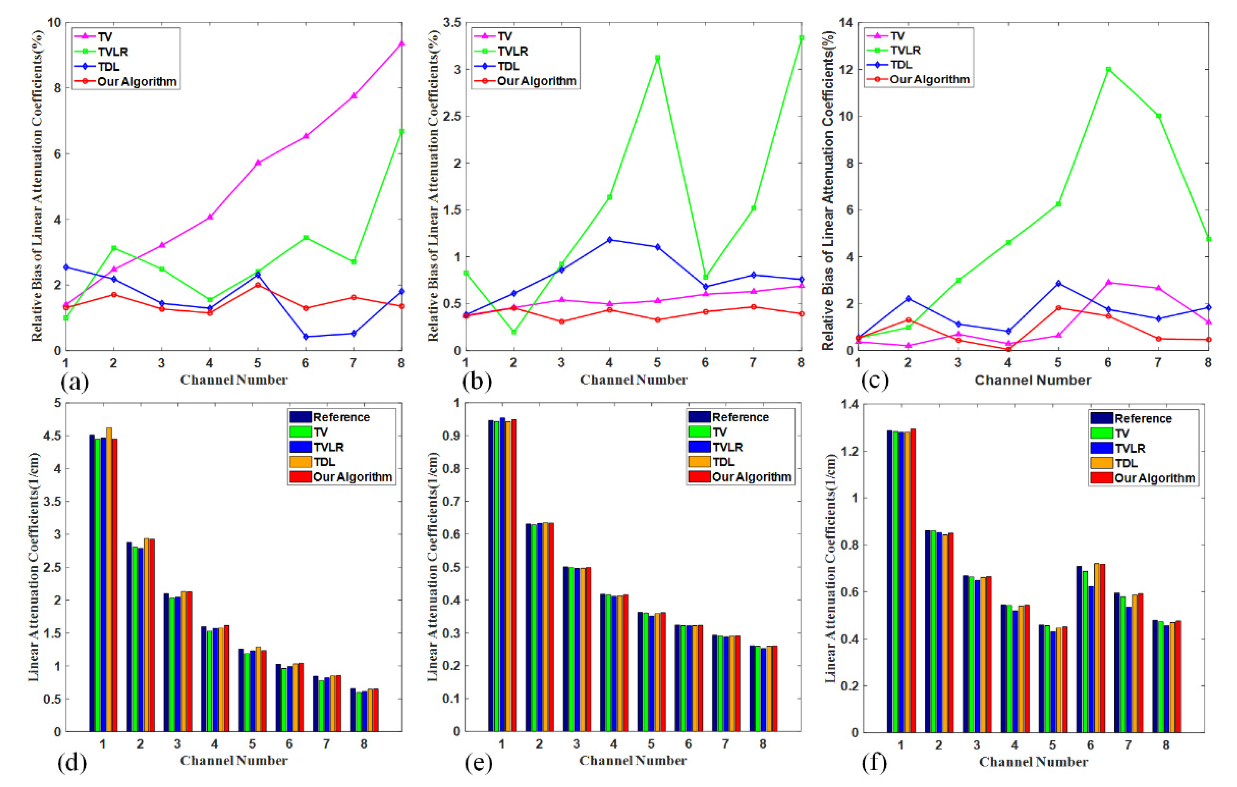
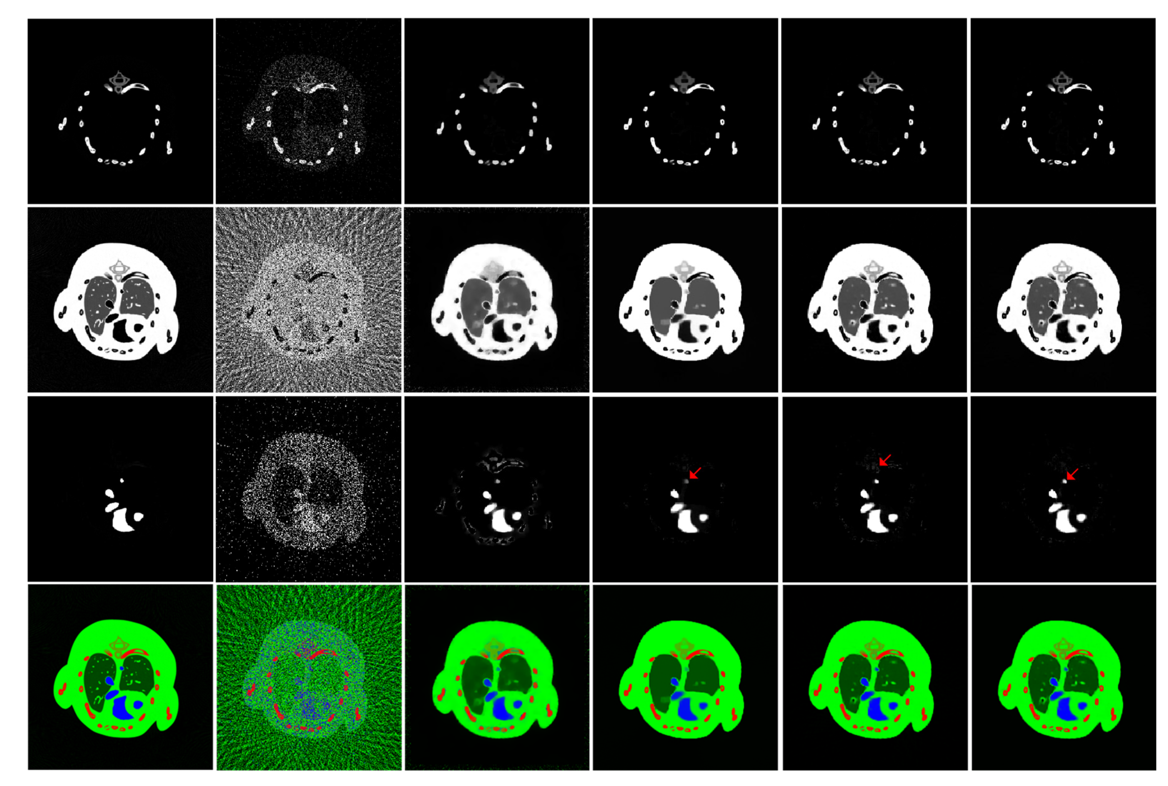
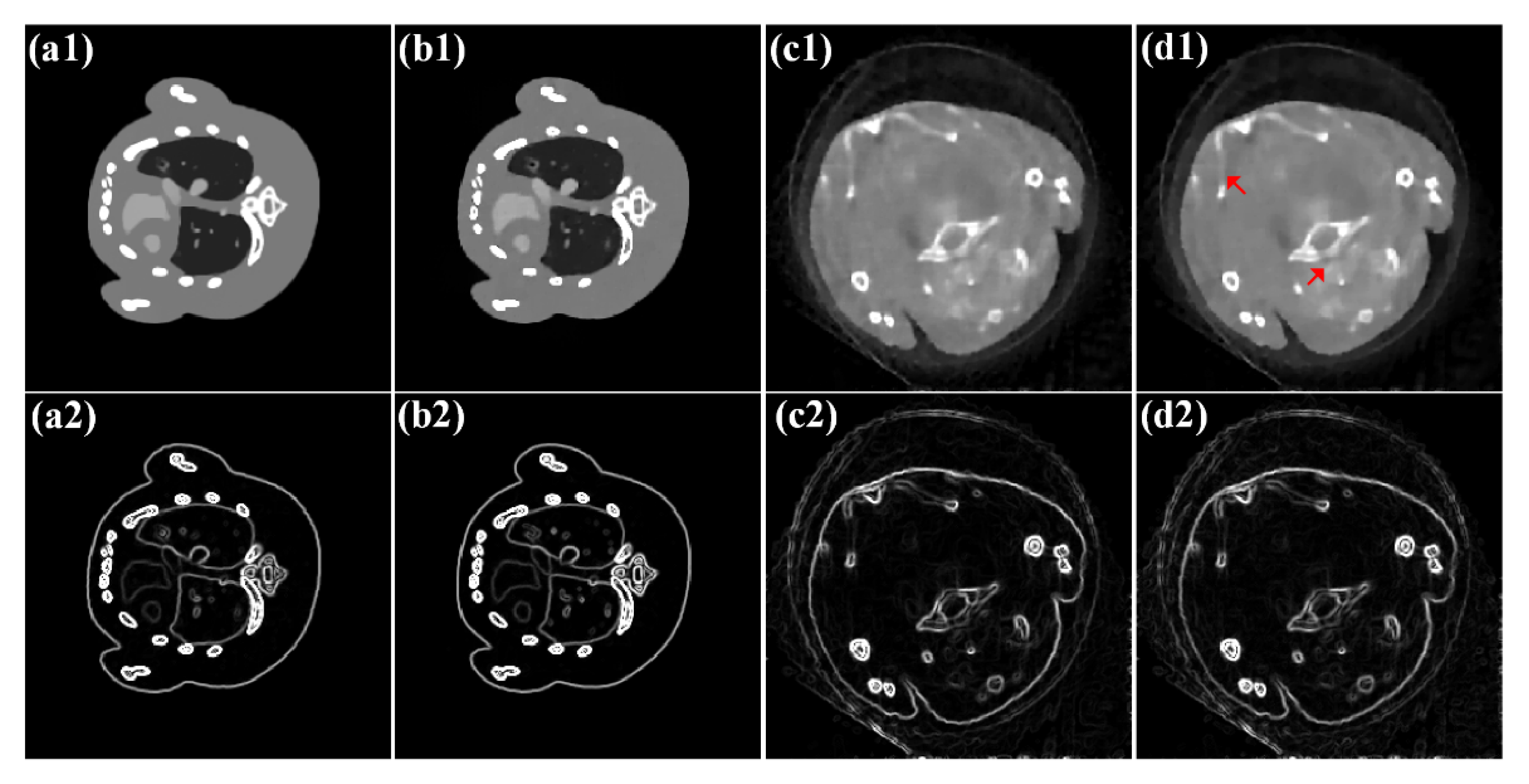
4.1. Numerical Simulation Study

In the simulation study, a digital mouse thoracic phantom with 1.2% iodine contrast agent added into the blood circulation, as shown in Figure 1a,b, is utilized to compare the results of all reconstruction methods. The voltage of the X-ray source is 50 kVp and the energy spectrum is divided into eight channels, [16, 22) keV, [22, 25) keV, [25, 28) keV, [28, 31) keV, [31, 34) keV, [34, 37) keV, [37, 41) keV, [41, 50) keV, as shown in Figure 1c. An equi-distant fan beam calculation is used. The distances from the X-ray source to the PCD are 180 mm, while the distances from the X-ray source to the rotation center are 132 mm. The detector system contains 512 units; each unit is 0.1 mm. Over a full scanning, 640 projections were collected. The reconstructed image tensor size is 256 × 256 × 8, where each pixel covers an area of 0.15 × 0.15 mm2. The number of photons in one X-ray path is 5000. In the numerical simulations, in order to quantitatively assess the image quality, the root mean square error (RMSE), structural similarity (SSIM) [43], and feature similarity (FSIM) [44] are calculated and compared.
To demonstrate the feasibility of the proposed algorithm for sparse-view projections in improving the quality of the reconstructed image, 160 and 80 views are extracted from a full scan. Ground truth images are reconstructed by the OS-SART algorithm with noise-free full scan projections. For briefness, this work only shows two representative energy channel such as the first and eighth channels. In this paper, the parameters have been optimized and selected through numerous experiments empirically. In the case of 160 projections, we set parameters as follows: ε = 1.3 × 10⁻³, a = 0.5, σ1 = 4.3, σ2 = 6.5, K = 1024, L = 11, η = 1.1. The reconstructed images from 160 views by using FBP, TV, TVLR, TDL, and our method are displayed in Figure 2. In Figure 2, the first row is the results of the different reconstruction methods for the first channel; the third row is for the eighth channel. To better compare the details of reconstructed images, we select the regions of interest (ROIs) and enlarge them to further display the results. The ROIs are marked by red and yellow boxes as shown in the first column in Figure 2. The enlarged results are shown in the second and fourth row of Figure 2. In the case of 80 projections, we set the parameters as follows: ε = 1.7 × 10⁻³, a = 0.5, σ1 = 6.2, σ2 = 9.1, K = 1024, L = 9, η = 1.3. The reconstructed images from 80 views by using different algorithms are shown in Figure 3. The first row is the results of the different reconstruction methods for the first channel; the third row is for the eighth channel. We also select the same position of ROIs and enlarge them for different algorithms.
From Figure 2 and Figure 3, we can intuitively get the conclusion that our algorithm is good at preserving image edge and recovering image finer structure than other algorithms. Concretely speaking, the results reconstructed from the FBP algorithm contain serious noise and obvious artifacts, as shown in (b1,b2). TV and TVLR results suffer from the image blurring and details missing as shown in (c1,c2) and (d1,d2). The results of TDL are better than the other methods as shown in (e1,e2). Yet from (f1,f2), it could be seen that our approach does well in maintaining subtle details and suppressing the noise effectively. The results can be clearly observed in the ROIs by the arrows, which point out some small image structures.
To facilitate comparison of the numerical accuracy of reconstructed images, we compare the image profiles of two representative regions, which are shown as a red line and a yellow line in Figure 1 left, to verify the accuracy of different algorithms in reconstructing images. The analysis results from 80 views are shown in Figure 4. The first and second rows are the first and eighth channels, respectively. From the first column to the last column, the profile results are a red line and a yellow line in the reconstructed images. The comparison algorithm is displayed in the legend. From the Figure 4, we could observe that the image profile reconstructed by TV produces large oscillation, especially in the eighth channel. Other algorithms obtain better results than TV. However, from the two representative regions, it could be observed that our algorithm has the best reconstruction accuracy.
To further demonstrate the superiority of our algorithm in preserving image edge and recovering subtle structures clearly, we compare gradients of the reconstructed images from 80 views, as shown in Figure 5. The first row is the first energy channel and the second row is the eighth energy channel. We select the region of edge changed dramatically as the ROIs, which are marked by the yellow rectangle. From the magnified ROIs, it could be observed that our method obtains better performance in edge preservation, especially in the eighth energy channel as pointed out by the green arrow. The red arrow shows a minor structure, it can be observed that our method dose well in recovering it both low energy channel and high energy channel. In order to compare algorithms from numerical indicators, we utilize three common indicators to evaluate such as RMSE, SSIM, and FSIM. The results are displayed in Table 1. From the Table, it can be clearly observed that the proposed algorithm has a better performance among the three indicators, which further demonstrates the superiority of our method.
Figure 6 displays the mean value and relative deviation of each channel in the bone, soft tissue, and iodine-enhanced areas for the selected iterative reconstruction method. For simplicity, we only show the results for 80 views. The relative deviation is computed as the absolute deviation divided by the average value of the corresponding reference value in the energy channel. The reference mean values of tissues (bone, soft, and iodine) are computed by the FBP algorithm from noise-free projection data. The TV algorithm smooths subtle structures in the bone regions and causes the largest relative deviation (up to 9.3% in channel 8), followed by TVLR (6.7% in channel 8). The proposed method achieves the most accurate and the relative deviations, which are below about 2% in all channels. The next one is the TDL method. For the soft tissues, TVLR gets the largest relative deviation with 3.3% in channel 8, followed by TDL with 0.65%. Meanwhile our algorithm and the TV algorithm are only below 0.62%. Regarding the iodine contrast agent, it can be seen from (c) that TVLR has the greatest relative deviation in channel 6 with 12%, due to the spectral flattening effect near the K-edge of iodine. The values from other algorithms are no more than 3%. In particular, the relative deviations of iodine from the proposed algorithm are below 2%.
In addition, to validate the competence of the proposed algorithm for material decomposition, the reconstructed spectral CT images from 80 views by FBP, TV, TVLR, TDL, and our algorithm are decomposed into three basis materials (bone, soft tissue, and iodine contrast agent) utilizing the material decomposition algorithm based on the image domain [45]. Figure 7 displays the decomposed results and the corresponding color images. It is observed from the third row that our method and TDL achieve the best accurate iodine regions, while other methods wrongly classify some pixels as iodine components. However, for the soft tissues, it is seen from the second row that the performance of our method is better than other competing methods.

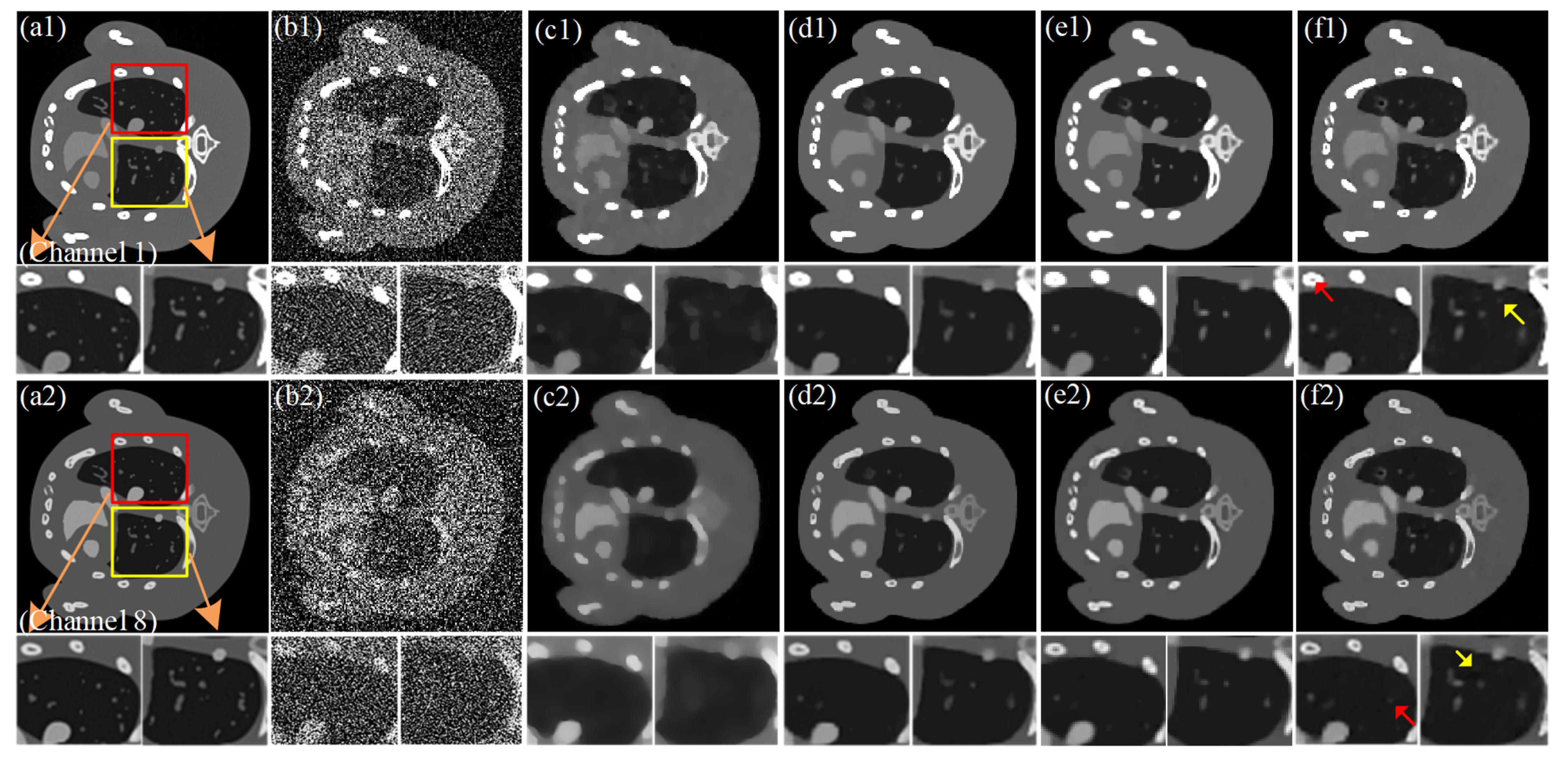
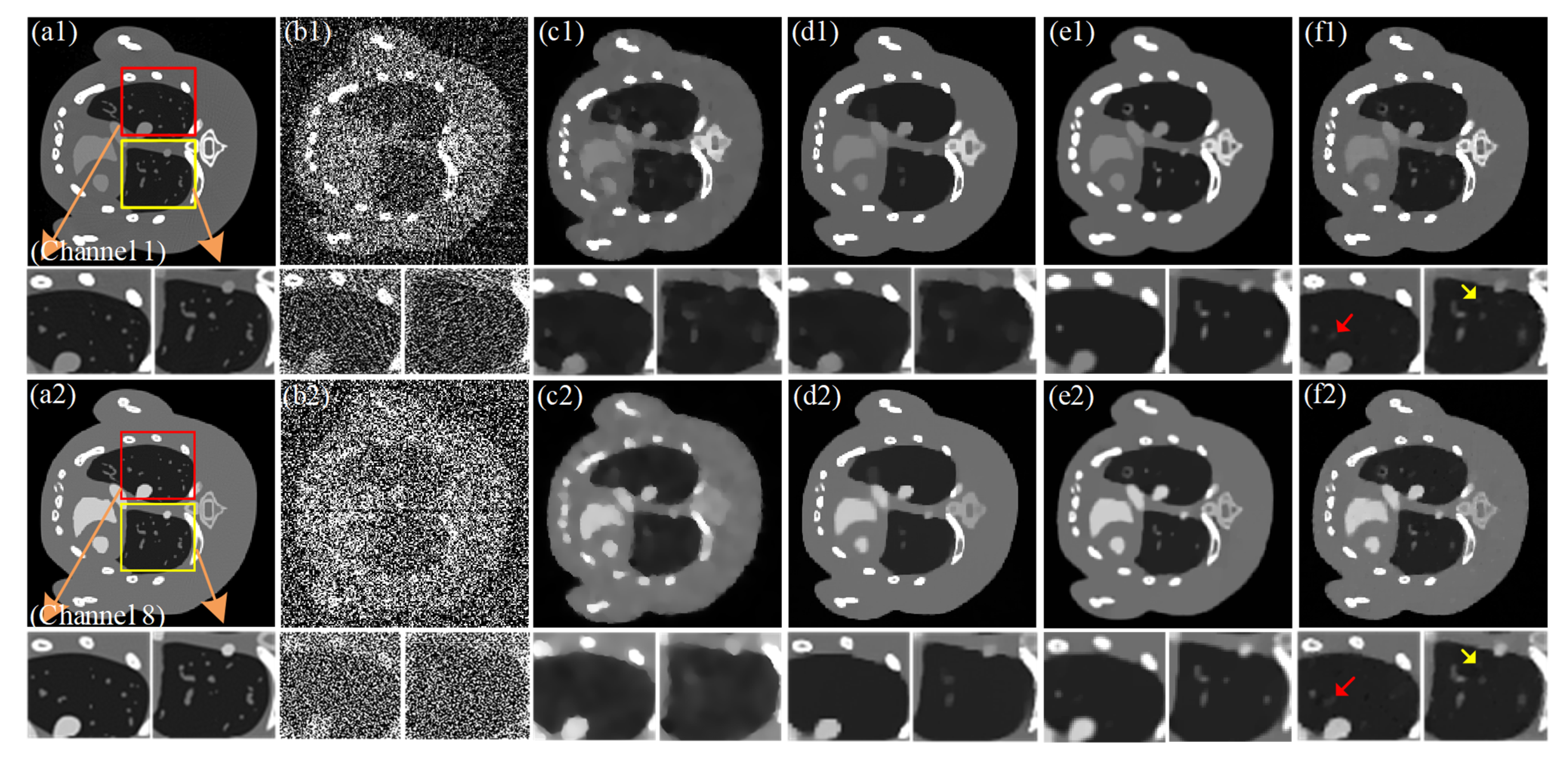
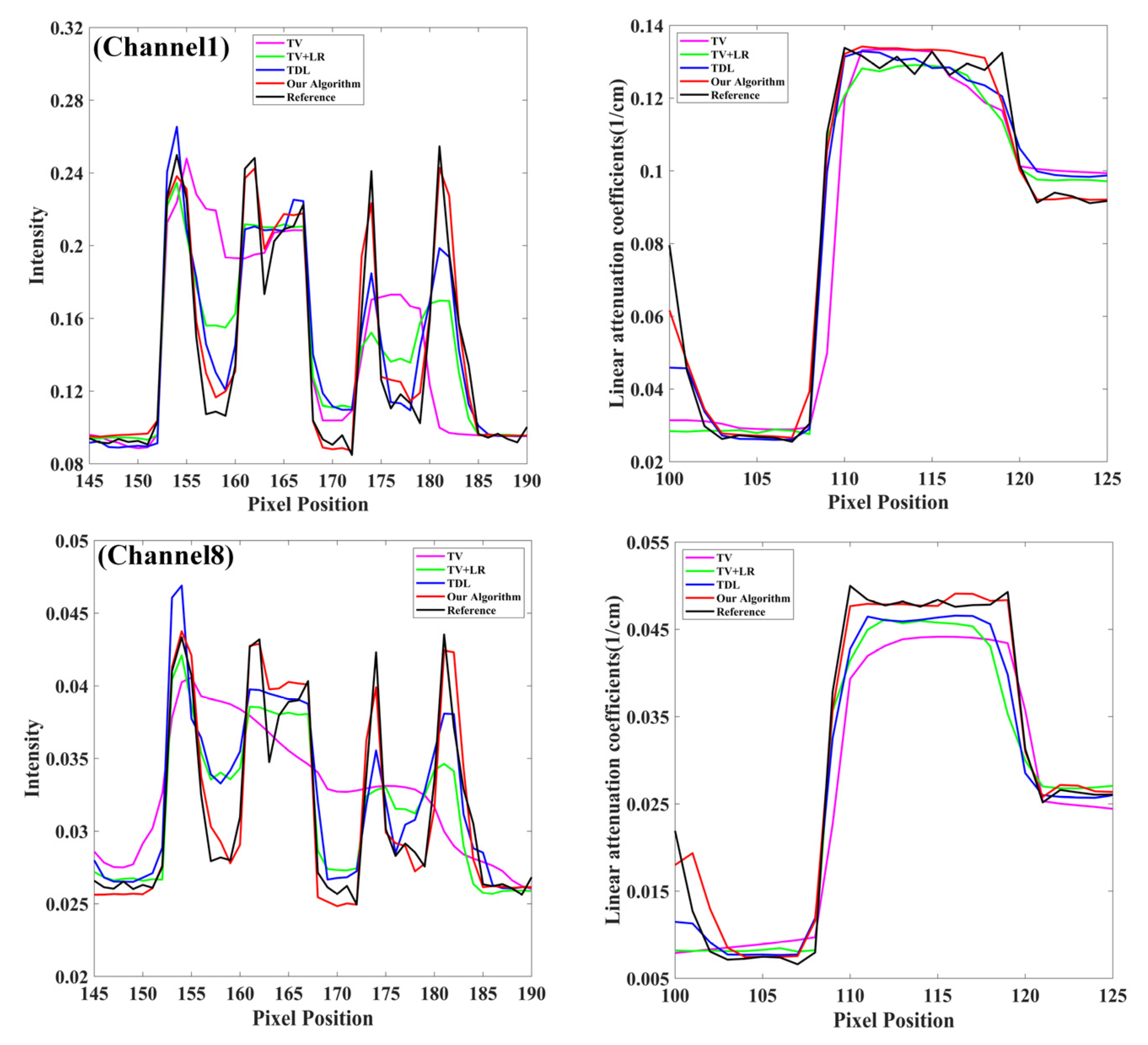
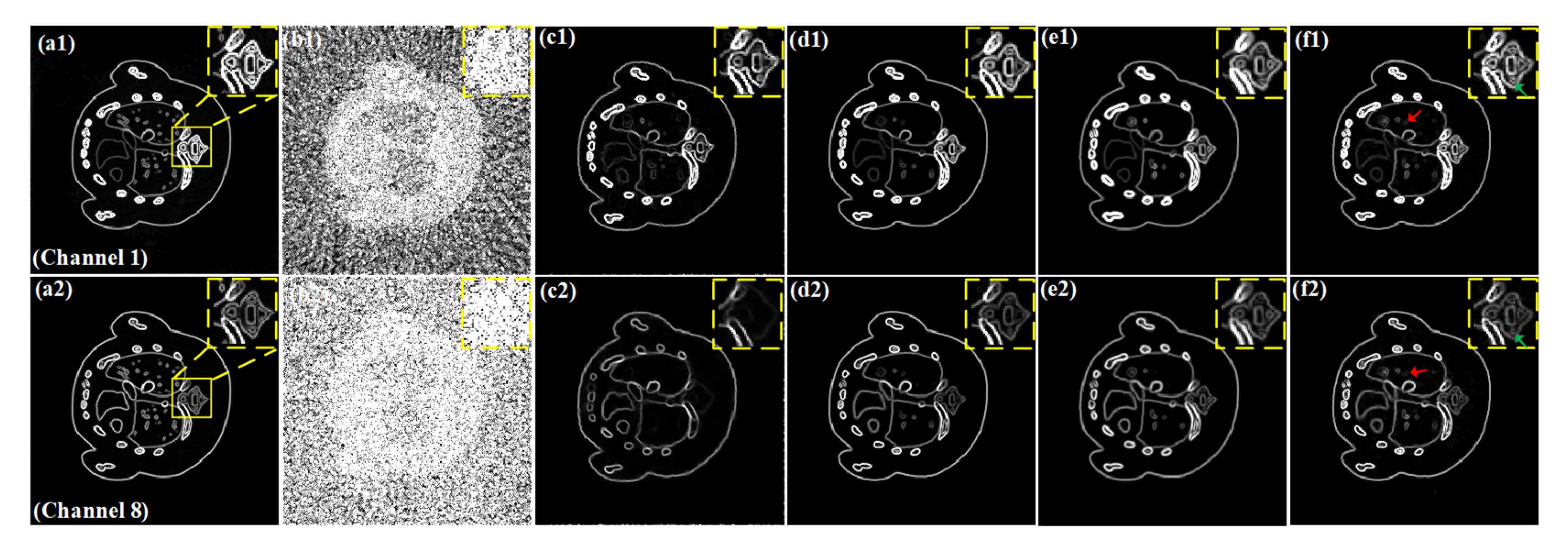
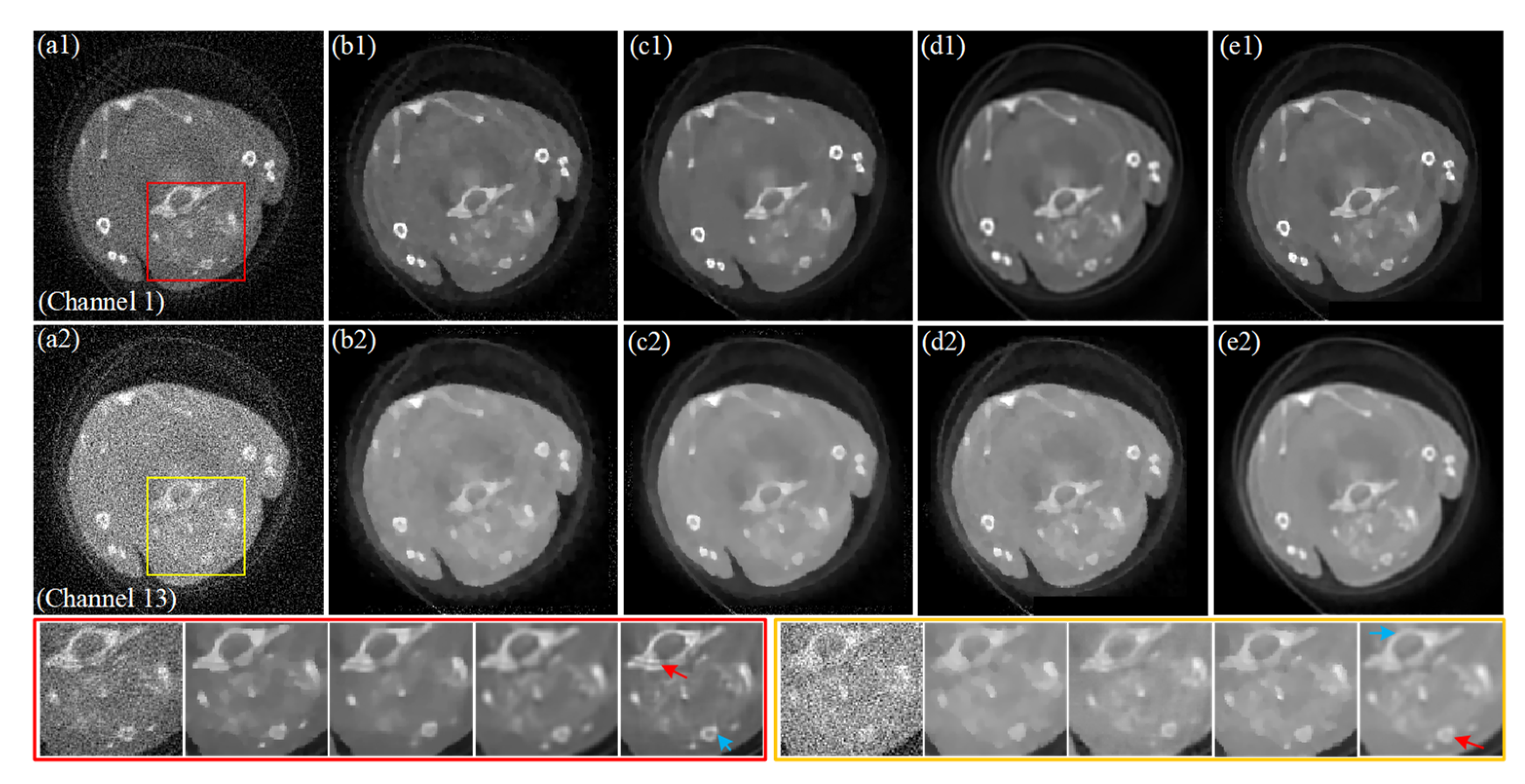
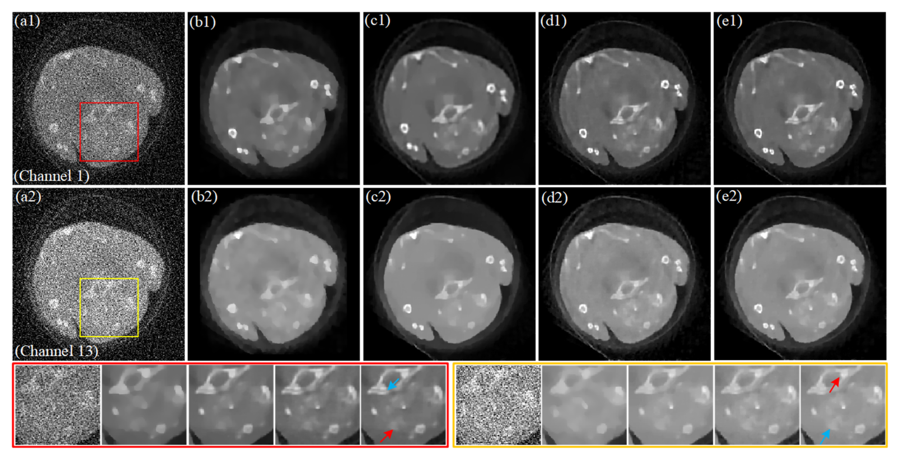
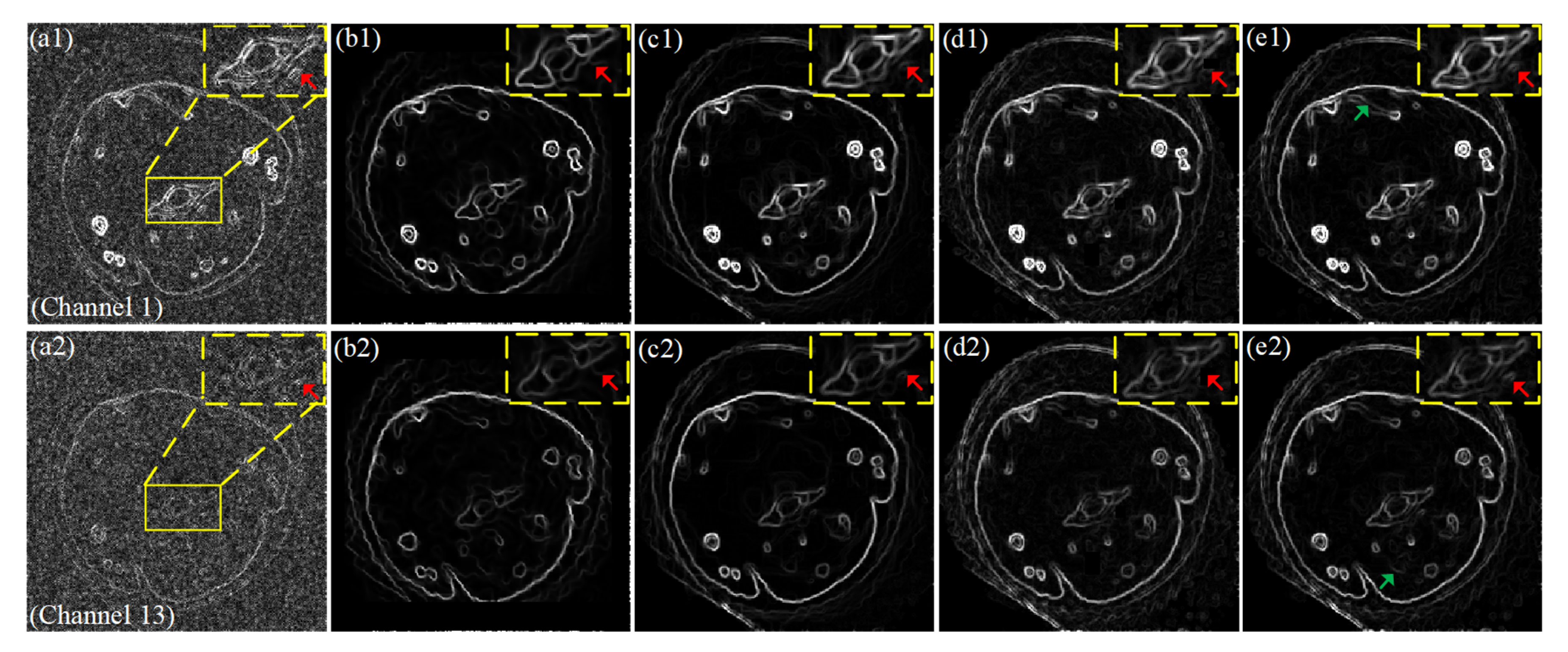
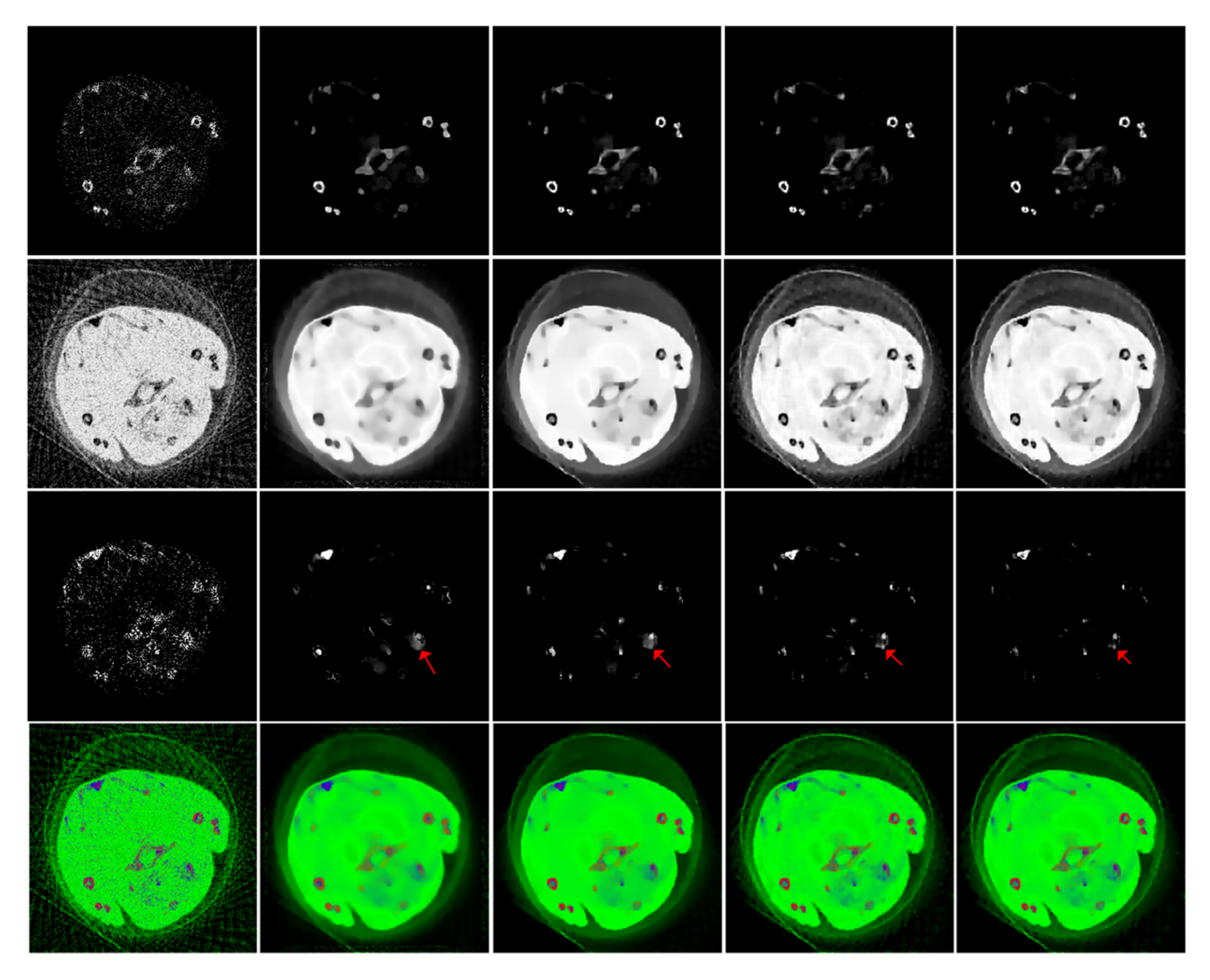
4.2. Preclinical Mouse Study

To show the advantages of the proposed algorithm, we further perform it in the practical application from a mouse injected with 0.2 mL of 15 nm Aurovist II gold nanoparticles (GNP) (Nanoparticles; Yaphank, NY, USA). The CT system includes an X-ray source and a photon counting detector. The distance from the X-ray source to the PCD is set as 255 mm, the distance from the X-ray source to the rotation centre is set as 158 mm. In a full scanning, 371 projections were evenly received. The 120 kVp energy spectrum of the X-ray source is divided into 13 channels. The channels of practical datasets were different from the datasets in numerical simulation. More specifically, here the X-ray photons are received by each energy channel only if the channel energy is higher than a certain energy threshold. Therefore, the first channel has the lowest energy threshold and almost contains all the photons, while the last channel has the least photons. The detector row contains 1024 elements, and the unit length is 55 µm. The diameter of the covered field of view (FOV) is 34.68 mm. To decrease noise in the sinogram, it is helpful to merge the adjacent detector bins to form a new sinogram of size 512 × 371. The reconstructed CT images were three-order tensors of 256 × 256 × 13, with an area of 18.41 × 18.41 mm2. We only show two representative channel images (channels 1 and 13) in the next experiment.
To validate the feasibility of the proposed algorithm for sparse view projections, 120 and 60 views are extracted from a full scan. In the case of 120 views, we set the parameters as follows: ε = 7 × 10⁻⁴, a = 0.5, σ1 = 3.5, σ2 = 5.7, K = 1024, L = 12, η = 1.1. The reconstructed results of the FBP, TV, TVLR, TDL, and our algorithm are displayed in Figure 8. The first row is the results for channel 1 and the second row is the results for channel 13. The last row is the corresponding regions of interest (ROIs) from (a1) to (e2) in sequence. In the case of 60 projections, we set the parameters as follows: ε = 8 × 10⁻⁴, a = 0.5, σ1 = 6.4, σ2 = 8.3, K = 1024, L = 10, η = 1.5. The reconstructed images of the FBP, TV, TVLR, TDL, and our algorithm are displayed in Figure 9. The first and second rows are the results for channels 1 and 13, respectively. The last row is the corresponding ROIs from (a1–e2) in sequence. The columns are the different reconstruction algorithms. From Figure 8 and Figure 9, it could be observed that the images obtained by the FBP algorithm have serious noise as shown in (a1,a2). The results of TV and TVLR contain blurry edges as shown in (b1,b2) and (c1,c2). The result of the TDL algorithm improves the image quality to some extent, yet some details are lost as displayed in (d1,d2). Obviously, the result of the proposed algorithm not only preserves the image edge, but also recovers finer image structures as shown in (e1,e2).
In order to better compare the details of reconstructed images, we select the ROIs and enlarge them to further display the results. The ROIs are marked by red and yellow boxes as shown in the first column in Figure 8 and Figure 9. The results are shown in the last row of (a1–e2) in sequence. From the magnified ROIs, we can observe that our algorithm can achieve the best results in recovering the finer image structures pointed out by the red and blue arrows, while it is difficult to distinguish the images reconstructed by the FBP, TV, TVLR, and TDL methods. Meanwhile, the ability of our algorithm to preserve image edge is better than other methods.
To further demonstrate the superiority of our algorithm in practical application clearly, we compare gradients of the reconstructed images from 60 views as shown in Figure 10. The first row is the first energy channel and the second row is the 13th energy channel. The first column is the reconstructed images from full projections utilizing FBP. We mark the ROIs by the yellow rectangle. From the enlarged ROIs, it could be seen that our algorithm obtains better performance in noise reduction and edge preservation, especially in the 13th energy channel, as pointed out by the green arrow shown in (e1,e2). The red arrow shows a minor structure; it can be seen that our method does well in recovering it concerning both low energy channel and high energy channel. Figure 11 shows the results of three basis material decomposition and the corresponding color images from 60 projections. As far as GNP components are concerned, it could be seen that our algorithm has fewer errors in misclassifying bone pixels as GNP regions indicated by the red arrows. On the whole, our algorithm is better than other competing algorithms in material decomposition, as seen from the color images.

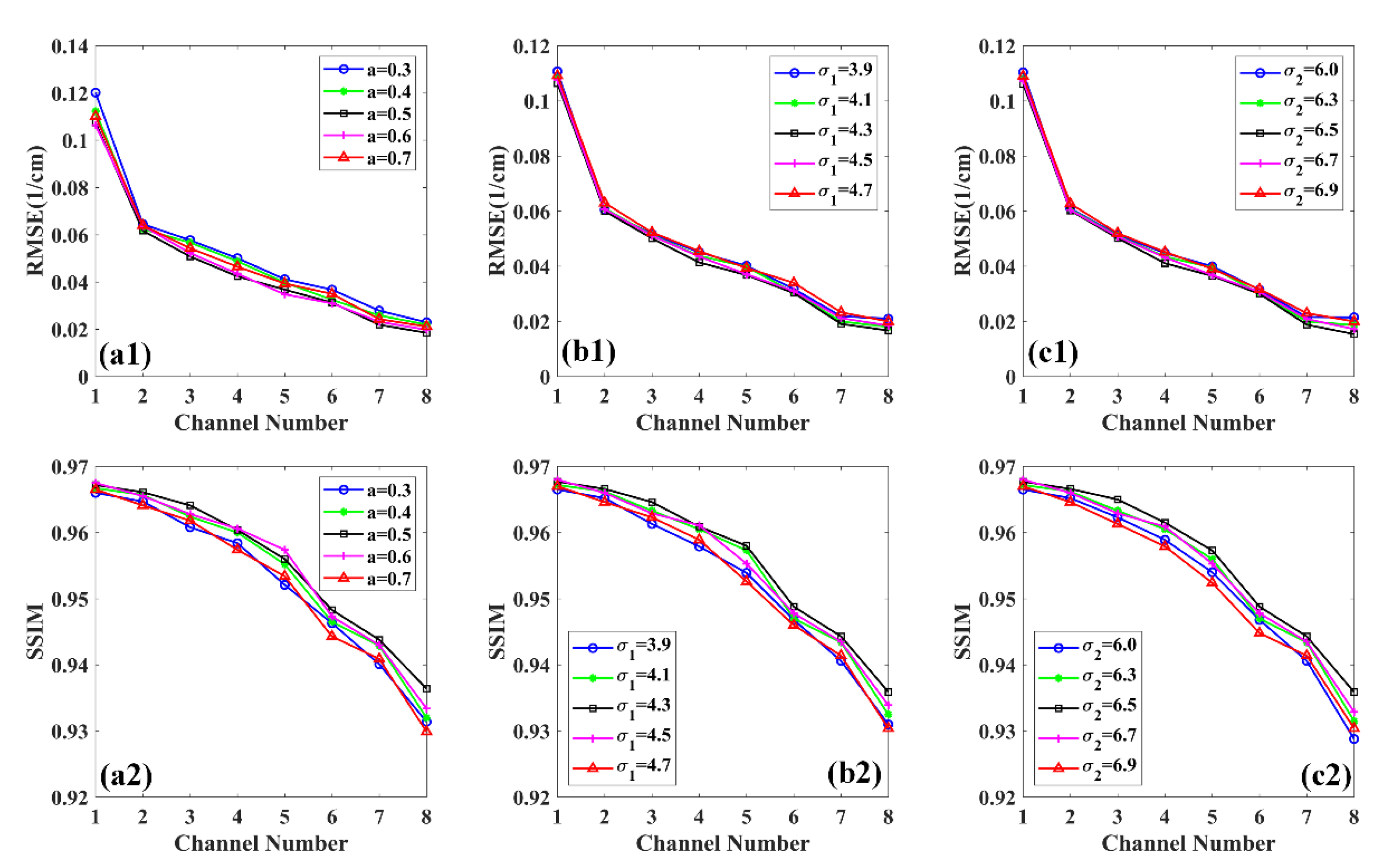
4.3. Parameters Analysis

It is challenging to determine the optimal parameters in iterative reconstruction algorithms for CT reconstruction. In the proposed method, the objective function in Equation (6) contains two regularization terms which need a number of parameters to optimize. Firstly, the parameters of the TDL term mainly contain precision level ε, sparse level L, atom number K, and regularization parameter η. In the paper by [30], it is very clear to illustrate the impact related to these parameters. In summary, a smaller ε can cause noise structure, while larger ones can damage the structural details. η controls the relationship among different channels, the larger η is, the stronger the relationship is, the smoother the image is. With regard to L, the smaller value will result in blurred edge. K is not sensitive to the reconstruction quality, which is set as 1024. We utilize the conclusion and optimize the parameter selection empirically. Here, we mainly focus on the second regularization term gradient L0-norm because the control factors a, σ1, and σ2 have a bigger impact on image quality compared with η in the TDL regularization term. Different settings of these parameters could lead to different quality of reconstructed images. In order to study the performance of our algorithm under different parameters, we only relax one or two free parameters while fixing other parameters. We go through numerous experiments and observe the changes of image quality with parameters. Figure 12 shows the RMSE and SSIM of the proposed algorithm with respect to different parameters. It can be seen that when a is 0.5, the RMSE and SSIM achieve the best value. σ1 and σ2 control the quality of reconstructed images. Smaller values will lead to noisy image, while larger values will over-smooth the edge structures. The figure shows the change of σ1 and σ2; it can be observed that when the values increase, the RMSE will be lower and SSIM will be higher, but if the values continue to increase, the indicators will obtain unsatisfactory results.

5. Discussion and Conclusions

In this study, to solve the limitation of the existing TDL-based spectral CT reconstruction method and further improve the reconstructed image quality, we propose a method termed TDL with an enhanced sparsity constraint for spectral CT reconstruction. The proposed algorithm inherits the advantage of TDL by exploring the correlation of spectral CT images from different channels. Moreover, the method designs a regularization using the L0-norm of the image gradient to constrain images and difference between images and a prior image in each energy channel simultaneously. Compared with the image gradient L1-norm, the image gradient L0-norm calculates the number of non-zero pixels instead of penalizing the large image gradient magnitudes. Therefore, it is more suitable to protect edge information. It is noted that the prior image used in our work is the total image reconstruction from all energy channels’ projection data, which plays an important role in the reconstruction process. Due to the similarity between a high-quality full-spectrum image and the target image, by incorporating the guidance of a prior image in each energy channel into the reconstruction model, the image quality is significantly improved, especially in the case of the sparse view problem. A natural question is how much contribution does the prior image have on the reconstruction images. To clearly show the contribution of the prior image, we also implemented the TDL with only L0-norm and compared it with our algorithm. Figure 13 shows the results of TDL with only L0-norm and our algorithm. From the figure, we can easily find that if a prior image is introduced to guide the reconstruction, more subtle structures will be preserved whether in simulation data or real data.
While better results have been obtained by utilizing the method, there are still some issues existing. Firstly, there are numerous parameters that need to be determined. This paper selects the optimal parameters empirically through a lot of experiments. Therefore, how to optimize parameters automatically is still an open problem that needs to be explored. In addition, the high quality of the global tensor dictionary and prior image are often not available in some cases. As a result, we have to utilize low-quality reconstructed images to train the global tensor dictionary and form a prior image, which may affect the final quality of the image. The problem of these cases will be investigated in our future work.
In conclusion, we propose a TDL with an enhanced sparsity constraint method for spectral CT reconstruction The proposed algorithm can not only eliminate noise, but also well preserve edge information and recover image details. The experimental results confirm that the performance of our algorithm is better than that of the TV, TVLR, and TDL methods.

Author Contributions

Conceptualization, X.L.; methodology, X.L.; software, X.L. and Y.Z.; validation, X.L. and X.S.; formal analysis, X.L.; data curation, Y.Z.; writing—original draft preparation, X.L. and X.S.; writing—review and editing, X.L. and P.C.; supervision, X.L. and J.P.; project administration, J.P. and P.C.; funding acquisition, P.C. All authors have read and agreed to the published version of the manuscript.

Funding

This research was funded by National Natural Science Foundation of China: 62122070, 61871351, 61971381; Shanxi Agricultural University Young Science and Technology Innovation Program: 2019021.

Institutional Review Board Statement

Not applicable.

Informed Consent Statement

Not applicable.

Data Availability Statement

Data underlying the results presented in this paper are not publicly available but may be obtained from the authors upon reasonable request.

Acknowledgments

The authors would like to thank the MARS team in New Zealand for the realistic mouse datasets. The authors are grateful to the anonymous reviewers for their valuable comments.

Conflicts of Interest

The authors declare no conflict of interest.

References

  1. Wang, G.; Yu, H.; De Man, B. An outlook on X-ray CT research and development. Med. Phys. 2008, 35, 1051–1064. [Google Scholar] [CrossRef] [Green Version]
  2. Nakano, M.; Haga, A.; Kotoku, J.; Magome, T.; Masutani, Y.; Hanaoka, S.; Kida, S.; Nakagawa, K. Cone-beam CT reconstruction for non-periodic organ motion using time-ordered chain graph model. Radiat. Oncol. 2017, 12, 1–14. [Google Scholar] [CrossRef]
  3. Brooks, R.A.; Di Chiro, G. Beam hardening in X-ray reconstructive tomography. Phys. Med. Biol. 1976, 21, 390–398. [Google Scholar] [CrossRef]
  4. Zhao, W.; Li, D.; Niu, K.; Qin, W.; Peng, H.; Niu, T. Robust Beam Hardening Artifacts Reduction for Computed Tomography Using Spectrum Modeling. IEEE Trans. Comput. Imaging 2018, 5, 333–342. [Google Scholar] [CrossRef]
  5. Brenner, D.J.; Hall, E.J. Computed tomography—An increasing source of radiation exposure. N. Engl. J. Med. 2013, 357, 2277–2284. [Google Scholar] [CrossRef] [Green Version]
  6. Nikzad, S.; Pourkaveh, M.; Vesal, N.J.; Gharekhanloo, F. Cumulative radiation dose and cancer risk estimation in common diagnostic radiology procedures. Iran. J. Radiol. 2018, 15, 60955. [Google Scholar] [CrossRef]
  7. Lee, T.S.; Tsui, B. Task-Based Evaluation of Image Reconstruction Methods for Defect Detection and Radiation Dose Reduction in Myocardial Perfusion SPECT. IEEE Trans. Radiat. Plasma Med. Sci. 2018, 3, 89–95. [Google Scholar] [CrossRef]
  8. Wang, Q.; Zhu, Y.; Yu, H. Locally linear constraint based optimization model for material decomposition. Phys. Med. Biol. 2017, 62, 8314–8340. [Google Scholar] [CrossRef]
  9. Wang, M.; Zhang, Y.; Liu, R.; Guo, S.; Yu, H. An adaptive reconstruction algorithm for spectral CT regularized by a reference image. Phys. Med. Biol. 2016, 61, 8699–8719. [Google Scholar] [CrossRef]
  10. Taguchi, K.; Iwanczyk, J.S. Vision 20/20: Single photon counting X-ray detectors in medical imaging. Med. Phys. 2013, 40, 100901. [Google Scholar] [CrossRef]
  11. Xi, Y.; Chen, Y.; Tang, R.; Sun, J.; Zhao, J. United iterative reconstruction for spectral computed tomography. IEEE Trans. Med. Imaging 2015, 34, 769–778. [Google Scholar] [CrossRef]
  12. Xu, Q. Image reconstruction for hybrid true-color micro-CT. IEEE Trans. Biomed. Eng. 2012, 59, 1711. [Google Scholar] [CrossRef] [Green Version]
  13. Liu, H.; Ge, W.; Yu, H.; Lei, X.; Xu, Q. Dictionary Learning Based Reconstruction with Low-Rank Constraint for Low-Dose Spectral CT. Med. Phys. 2016, 43, 3701. [Google Scholar]
  14. Wu, W.; Yu, H.; Chen, P.; Luo, F.; Liu, F.; Wang, Q.; Zhu, Y.; Zhang, Y.; Feng, J.; Yu, H. Dictionary learning based image-domain material decomposition for spectral CT. Phys. Med. Biol. 2020, 65, 245006. [Google Scholar] [CrossRef]
  15. Kong, H.; Lei, X.; Lei, L.; Zhang, Y.; Yu, H. Spectral CT Reconstruction Based on PICCS and Dictionary Learning. IEEE Access 2020, 8, 133367–133376. [Google Scholar] [CrossRef]
  16. Zhao, B.; Gao, H.; Ding, H.; Molloi, S. Tight-frame based iterative image reconstruction for spectral breast CT. Med. Phys. 2013, 40, 031905. [Google Scholar] [CrossRef]
  17. Kim, K.; Ye, J.C.; Worstell, W.; Ouyang, J.; Rakvongthai, Y.; Fakhri, G.E.; Li, Q. Sparse-view spectral CT reconstruction using spectral patch-based low-rank penalty. IEEE Trans. Med. Imaging 2015, 34, 748–760. [Google Scholar] [CrossRef]
  18. Chu, J.; Cong, W.; Li, L.; Wang, G. Combination of current-integrating/photon-counting detector modules for spectral CT. Phys. Med. Biol. 2013, 58, 7009–7024. [Google Scholar] [CrossRef]
  19. Rigie, D.S.; La Rivière, P.J. Joint reconstruction of multi-channel, spectral CT data via constrained total nuclear variation minimization. Phys. Med. Biol. 2015, 60, 1741–1762. [Google Scholar] [CrossRef] [Green Version]
  20. Semerci, O.; Hao, N.; Kilmer, M.E.; Miller, E.L. Tensor-based formulation and nuclear norm regularization for multienergy computed tomography. IEEE Trans. Image Process. 2014, 23, 1678–1693. [Google Scholar] [CrossRef] [Green Version]
  21. Gao, H.; Yu, H.; Osher, S.; Wang, G. Multi-energy CT based on a prior rank, intensity and sparsity model (PRISM). Inverse Probl. 2011, 27, 115012. [Google Scholar] [CrossRef] [Green Version]
  22. Liang, L.; Chen, Z.; Wang, G.; Chu, J.; Gao, H. A tensor PRISM algorithm for multi-energy CT reconstruction and comparative studies. J. X-ray Sci. Technol. 2014, 22, 147–163. [Google Scholar]
  23. Wu, W.; Hu, D.; An, K.; Wang, S.; Luo, F. A High-Quality Photon-Counting CT Technique Based on Weight Adaptive Total-Variation and Image-Spectral Tensor Factorization for Small Animals Imaging. IEEE Trans. Instrum. Meas. 2021, 70, 1–14. [Google Scholar] [CrossRef]
  24. Wu, W.; Chen, P.; Vardhanabhuti, V.; Wu, W.; Yu, H. Improved Material Decomposition with a Two-step Regularization for spectral CT. IEEE Access 2019, 7, 158770–158781. [Google Scholar] [CrossRef]
  25. Hu, D.; Wu, W.; Xu, M.; Zhang, Y.; Liu, J.; Ge, R.J.; Chen, Y.; Luo, L.; Coatrieux, G. SISTER: Spectral-Image Similarity-Based Tensor with Enhanced-Sparsity Reconstruction for Sparse-View Multi-Energy CT. IEEE Trans. Comput. Imaging 2020, 6, 477–490. [Google Scholar] [CrossRef]
  26. Yu, Z.; Leng, S.; Li, Z.; Mccollough, C.H. Spectral prior image constrained compressed sensing (spectral PICCS) for photon-counting computed tomography. Phys. Med. Biol. 2016, 61, 6707. [Google Scholar] [CrossRef] [Green Version]
  27. Niu, S.; Zhang, Y.; Ma, J.; Wang, J. WE-FG-207B-05: Iterative Reconstruction Via Prior Image Constrained Total Generalized Variation for Spectral CT. Med. Phys. 2016, 43, 3835. [Google Scholar] [CrossRef]
  28. Wang, S.; Wu, W.; Feng, J.; Liu, F.; Yu, H. Low-dose spectral CT reconstruction based on image-gradient L0 -norm and adaptive spectral PICCS. Phys. Med. Biol. 2020, 65, 245005. [Google Scholar] [CrossRef]
  29. Xu, Q.; Yu, H.Y.; Mou, X.Q.; Zhang, L.; Hsieh, J.; Wang, G. Low-dose X-ray CT reconstruction via dictionary learning. IEEE Trans. Med. Imaging 2012, 31, 1682–1697. [Google Scholar] [CrossRef] [Green Version]
  30. Zhang, Y.; Mou, X.; Wang, G.; Yu, H. Tensor-Based Dictionary Learning for Spectral CT Reconstruction. IEEE Trans. Med. Imaging 2017, 36, 142–154. [Google Scholar] [CrossRef] [Green Version]
  31. Peng, Y.; Meng, D.; Xu, Z.; Gao, C.; Yang, Y.; Zhang, B. Decomposable nonlocal tensor dictionary learning for multispectral image denoising. In Proceedings of the 2014 IEEE Conference on Computer Vision and Pattern Recognition, Columbus, OH, USA, 23–28 June 2014; pp. 2949–2956. [Google Scholar] [CrossRef]
  32. Gong, X.; Chen, W.; Chen, J. A Low-Rank Tensor Dictionary Learning Method for Hyperspectral Image Denoising. IEEE Trans. Signal Process. 2020, 68, 1168–1180. [Google Scholar] [CrossRef]
  33. Tan, S.; Zhang, Y.; Wang, G.; Mou, X.; Cao, G.; Wu, Z.; Yu, H. Tensor-based dictionary learning for dynamic tomographic reconstruction. Phys. Med. Biol. 2015, 60, 2803–2818. [Google Scholar] [CrossRef] [Green Version]
  34. Wu, W.; Zhang, Y.; Wang, Q.; Liu, F.; Chen, P.; Yu, H. Low-dose spectral CT reconstruction using image gradient ℓ0–norm and tensor dictionary. Appl. Math. Model. 2018, 63, 538–557. [Google Scholar] [CrossRef]
  35. Li, X.; Lu, C.; Yi, X.; Jia, J. Image Smoothing via L0 Gradient Minimization. ACM Trans. Graph. 2011, 30, 1–12. [Google Scholar]
  36. Biswas, S.; Hazra, R. A new binary level set model using L0 regularizer for image segmentation. Signal Process. 2020, 174, 107603. [Google Scholar] [CrossRef]
  37. Yuan, G.; Ghanem, B. ℓ0 TV: A Sparse Optimization Method for Impulse Noise Image Restoration. IEEE Trans. Pattern Anal. Mach. Intell. 2019, 41, 352–364. [Google Scholar] [CrossRef] [Green Version]
  38. Duan, G.; Wang, H.; Liu, Z.; Deng, J.; Chen, Y.W. K-CPD: Learning of overcomplete dictionaries for tensor sparse coding. In Proceedings of the 21st International Conference on Pattern Recognition (ICPR2012), Tsukuba, Japan, 11–15 November 2012; pp. 493–496. [Google Scholar]
  39. Boyd, S.; Parikh, N.; Chu, E.; Peleato, B.; Eckstein, J. ADMM slide. Found. Trends Mach. Learn. 2010, 3, 1–122. [Google Scholar] [CrossRef]
  40. Liu, Q.; Liang, D.; Song, Y.; Luo, J.; Zhu, Y.; Li, W. Augmented lagrangian-based sparse representation method with dictionary updating for image deblurring. SIAM J. Imaging Sci. 2013, 6, 1689–1718. [Google Scholar] [CrossRef]
  41. Yu, W.; Wang, C.; Huang, M. Edge-preserving reconstruction from sparse projections of limited-angle computed tomography using ℓ0-regularized gradient prior. Rev. Sci. Instrum. 2017, 88, 043703. [Google Scholar] [CrossRef]
  42. Ren, D.; Zhang, H.; Zhang, D.; Zuo, W. Fast total-variation based image restoration based on derivative alternated direction optimization methods. Neurocomputing 2015, 170, 201–212. [Google Scholar] [CrossRef]
  43. Wang, Z.; Bovik, A.C.; Sheikh, H.R.; Simoncelli, E.P. Image quality assessment: From error visibility to structural similarity. IEEE Trans. Image Process. 2004, 13, 600–612. [Google Scholar] [CrossRef] [PubMed] [Green Version]
  44. Zhang, L.; Zhang, L.; Mou, X.; Zhang, D. FSIM: A Feature Similarity Index for Image Quality Assessment. IEEE Trans. Image Process. 2011, 20, 2378–2386. [Google Scholar] [CrossRef] [PubMed] [Green Version]
  45. Wu, W.; Chen, P.; Wang, S.; Vardhanabhuti, V.; Liu, F.; Yu, H. Image-Domain Material Decomposition for Spectral CT Using a Generalized Dictionary Learning. IEEE Trans. Radiat. Plasma Med. Sci. 2021, 5, 537–547. [Google Scholar] [CrossRef] [PubMed]
Figure 1. (a) Mice thorax phantom, (b) iodine contrast agent, (c) spectrum curve.
Photonics 09 00035 g001
Figure 2. Reconstructed images from 160 projections using different methods. The first two rows are the first channel and ROIs, the last two rows are the eighth channel and ROIs. From left to right, the columns are Ground Truth (a), FBP (b), TV (c), TVLR (d), TDL (e), and our algorithm (f). The display windows are [0, 0.25] cm−1 and [0, 0.08] cm−1, respectively.
Photonics 09 00035 g002
Figure 3. Reconstructed images from 80 projections using different methods. The first two rows are the first channel and ROIs, the last two rows are the eighth channel and ROIs. From left to right, the columns are Ground Truth (a), FBP (b), TV (c), TVLR (d), TDL (e), and our algorithm (f). The display windows are [0, 0.25] cm−1 and [0, 0.06] cm−1, respectively.
Photonics 09 00035 g003
Figure 4. Comparison of the profile from 80 views. The comparison algorithm is displayed in the legend.
Photonics 09 00035 g004
Figure 5. The gradient images from 80 views. The first row is the first energy channel and the second row is the eighth energy channel. From left to right, the columns are Ground Truth, FBP, TV, TVLR, TDL, and our algorithm. The display windows are [0, 0.08] cm−1 and [0, 0.02] cm−1.
Photonics 09 00035 g005
Figure 6. Mean values of three basic materials in each channel (bottom) and the corresponding relative bias (top). From left to right is bone (a,d), soft (b,e), and iodine contrast (c,f).
Photonics 09 00035 g006
Figure 7. Material decomposition results from 80 views. From top to bottom rows, the first three rows are the decomposed bone, soft tissues, and iodine contrast agent components, respectively. The fourth row is the color representation of the corresponding basic materials. From left to right, the columns are Ground truth, FBP, TV, TVLR, TDL, and our algorithm.
Photonics 09 00035 g007
Figure 8. Reconstructed images from 120 projections using different methods. The first and the second rows are the results for channels 1 and 13, respectively. The last row is the corresponding ROIs from (a1e2) in sequence. From left to right, the columns are FBP (a), TV (b), TVLR (c), TDL (d), and our algorithm (e). The display windows are [0, 0.1] cm−1 and [0, 0.08] cm−1, respectively.
Photonics 09 00035 g008
Figure 9. Reconstructed images from 60 projections using different methods. The first and the second rows are the results for channels 1 and 13, respectively. The last row is the corresponding ROIs from (a1e2) in sequence. From left to right, the columns are FBP (a), TV (b), TVLR (c), TDL (d), and our algorithm (e). The display windows are [0, 0.1] cm−1 and [0, 0.08] cm−1, respectively.
Photonics 09 00035 g009
Figure 10. The gradient images from 60 projections. The first row is the first channel and the second row is the 13th channel. The first column is an image reconstructed from full projections using the FBP algorithm (a). Other columns are TV (b), TV + LR (c), TDL (d), and our algorithm (e). The display windows are [0, 0.02] cm−1.
Photonics 09 00035 g010
Figure 11. Material decomposition results from 60 views. From top to bottom, the first three rows are the decomposed bone, soft tissues, and GNP components, respectively. The fourth row is the color representation of the corresponding basic materials. From left to right, the columns are FBP, TV, TVLR, TDL, and our algorithm.
Photonics 09 00035 g011
Figure 12. RMSE and SSIM analysis of different parameters: Parameter a (a), σ1 (b), σ2 (c).
Photonics 09 00035 g012
Figure 13. Comparison of the results of TDL with only L0-norm and our algorithm. The first row is the reconstruction results, the second row is the corresponding gradient images. (a,c) TDL with only L0-norm; (b,d) our algorithm.
Photonics 09 00035 g013
Table 1. Comparison of indicators in different angles using different methods.
ViewsChannelRMSESSIMFSIM
Method1st8th1st8th1st8th
80TV0.16460.04360.91670.87520.90360.8616
TVLR0.14880.03890.93020.90710.92140.8961
TDL0.14030.03220.93980.91280.92810.9024
Ours0.12160.02130.95010.92550.94580.9137
160TV0.14860.03720.93130.89820.92370.8863
TVLR0.13640.02830.94230.91230.93520.9014
TDL0.12510.02390.95280.92350.94260.9135
Ours0.10750.01870.96720.93640.95130.9308
Publisher’s Note: MDPI stays neutral with regard to jurisdictional claims in published maps and institutional affiliations.

