Article

Deformation Measurements of Neuronal Excitability Using Incoherent Holography Lattice Light-Sheet Microscopy (IHLLS)

1
Department of Anatomy and Cell Biology, University of Illinois at Chicago, 808 South Wood Street, Chicago, IL 60612, USA
2
Department of Applied Physics and Materials Science, Northern Arizona University, Flagstaff, AZ 86011, USA
3
Center for Materials Interfaces in Research and Development, Northern Arizona University, Flagstaff, AZ 86011, USA
*
Author to whom correspondence should be addressed.
Photonics 2021, 8(9), 383; https://doi.org/10.3390/photonics8090383
Submission received: 3 July 2021 / Revised: 1 September 2021 / Accepted: 2 September 2021 / Published: 9 September 2021
(This article belongs to the Special Issue Holography)

Abstract

:
Stimuli to excitable cells and various cellular processes can cause cell surface deformations; for example, when excitable cell membrane potentials are altered during action potentials. However, these cellular changes may be at or below the diffraction limit (in dendrites the structures measured are as small as 1 µm), and imaging by traditional methods is challenging. Using dual lenses incoherent holography lattice light-sheet (IHLLS-2L) detection with holographic phase imaging of selective fluorescent markers, we can extract the full-field cellular morphology or structural changes of the object’s phase in response to external stimulus. This approach will open many new possibilities in imaging neuronal activity and, overall, in light sheet imaging. In this paper, we present IHLLS-2L as a well-suited technique for quantifying cell membrane deformation in neurons without the actuation of a sample stage or detection microscope objective.

1. Introduction

Excitable cells, whether neurons or muscle cells, rapidly transport ions during excitation [1]. Excitation may be due to direct mechanical deformation in mechanoreceptive cells [2], or following, for example, rhodopsin activation for light receptors or G protein coupled olfactory receptors for olfaction [3]. In the central nervous system, excitation can follow the synaptic activation of ligand gated ion channels. Common to these processes, sensory or synaptic activation leads to transmembrane ion fluxes. These fluxes occur across the plasma membrane, and also across intracellular membranes when Ca2+ is released from internal stores. In excitable cells, depolarization of the plasma membrane is achieved by cation flux, including Na+ and K+ and Ca2+ ions. These processes ultimately lead to depolarization, and in excitable cells the explosive activation of voltage gated Na+ channels to cause an action potential. Neuronal excitation, whether sensory, synaptic, or part of the subsequent resulting action potentials, has been studied traditionally by intracellular electrophysiological recordings [4] and by fluorescence detection methods [5]. However, mechanical deformation in excitable cells occurs during action potential firing. This membrane deformation during an action potential is poorly understood, but the onset of cellular deformation coincides with the depolarization phase of the action potential [6]. At a theoretical level, thermodynamics predicts that transmembrane voltage modulates membrane tension and that this will cause movement [7]. Thus, modulation of membrane tension by transmembrane voltage in a neuron should cause movement of the membrane with magnitude and polarity governed by the cell membrane stiffness and surface potentials to maintain pressure across the membrane [8].
The currently available techniques to study cellular membrane dynamics include electrophysiological recording [9], fluorescence spectroscopy analysis [10], and optical imaging such as total internal reflection fluorescence microscopy (TIRFM) [11], quantitative phase imaging (QPI), and digital holography [12,13,14,15,16,17]. The electrophysiological recording method has limited throughput because it measures one cell at a time, and the fluorescence imaging signal does not provide direct information on the cell membrane mechanical deformation. Total internal reflection fluorescence microscopy (TIRFM) is commonly used to visualize the vesicle movement and fusion within a short distance of the evanescent field action. Digital holography and QPI are powerful three-dimensional (3D) imaging modalities because the sample volume is built from the complex-amplitude distribution [18]. At cell and tissue scale, resolutions in biomedicine, digital holography is used to provide experimental access to the quantitative phase of various cell types and tissues [19,20,21,22]; for example, to reconstruct blood cell movements [15,16], and to perform microsurgeries on cells [17]. All these techniques use coherent light, such as laser, which introduces extra noise from speckle and spurious interference that limit the imaging capabilities. A way to get around this issue is to use spatial incoherent light, such as fluorescent light, to form holograms, and produce images with better spatial resolution than conventional imaging [23].
Our new imaging technique [24], incoherent holography lattice light-sheet (IHLLS), provides the imaging capability to build the 3D complex amplitude volume of neurons with a resolution comparable or better than the conventional LLS’s resolution in dithering mode and with an extended FOV. IHHLS in both forms, with one diffractive lens, IHLLS 1L or two diffractive lenses with randomly selected pixels, IHLLS 2L, utilizes the excitation technology of the lattice light-sheet (LLS) system [25,26], in which excitation light is confined to a plane defined by a lattice of intersecting Bessel beams that self-reinforce as they project through tissue. The beam can be viewed orthogonally to its projection (Visualization 1 [24]), and the imaging detection uses the Fresnel incoherent correlation holography (FINCH) [27,28,29,30,31] principle. FINCH uses the self-interference property of the emitted fluorescent light to create Fresnel holograms of a 3D object in combination with the phase-shifting concept in which three or four interference patterns are created by a single channel on-axis interferometer. The beam splitter of the interferometer is replaced by a spatial light modulator (SLM), so that each spherical beam propagating from each 3D object’s points is split into two spherical beams with different radii of curvature. The interference patterns are added incoherently to further create Fresnel holograms. These holograms are numerically processed by in-house diffraction software.
IHLLS 1L is the incoherent version of the LLS in dithering mode, but the axial performance is perturbed by the lens of constant phase focusing to infinity. In IHLLS 2L, the z-galvanometric mirror is swept along the z-axis and the detection objective is kept fixed, reaching to certain depths through the phase modulation encoded in the two superposed Fresnel patterns.
Using our new technique, we will examine how a neuronal cell’s membrane shape changes by chemical stimuli that cause cell swelling.
This paper is organized as follows: In Section 2, the materials and methods are presented. Section 3 covers the FINCH technique with two diffractive lenses adapted for our new design and concept of IHLLS, as well as a series of experiments using neuronal cells. Finally, we make some concluding remarks and discussions in Section 4.

2. Materials and Methods
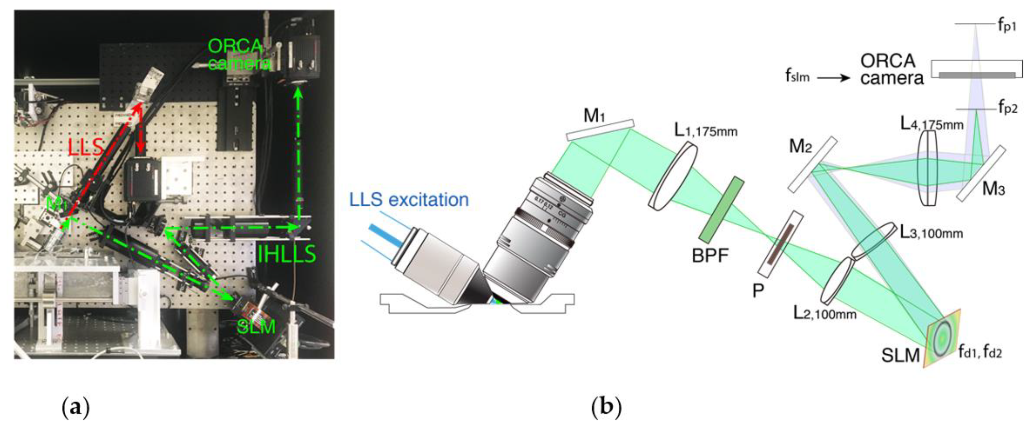
2.1. System Control

The entire system was controlled by the original LLS software based on LabView platform (National Instruments, Austin, TX, USA) with the diffractive SLM (Meadowlark Optics Inc., Longmont, CO, USA), synchronized with the ORCA camera for the IHLLS module. The complex hologram is propagated and reconstructed at the best focal plane using a custom diffraction method routine in MATLAB (MathWorks, Inc., Portola Valley, CA, USA).

2.2. Sample Preparation

Fluorescent latex beads of 500 nm λexc = 488 nm, λem = 520 nm, F-8888, (ThermoFisher Scientific, Waltham, MA, USA) were used as test objects [24]. The bead solution (2% solids) was diluted 1:4000 with distilled water and briefly centrifuged in a desktop centrifuge for 1 min. Clean coverslips were prepared by applying 1 µL of the bead solution as a thin layer that was left to dry. After drying, the cover slip with attached beads was mounted in the sample holder under distilled water.
Lamprey neurons were imaged in isolated spinal cords of newly transformed lampreys (Petromyzon marinus). The animals were anesthetized with tricaine methanesulfonate (MS-222; 100 mg/L; Sigma, St. Louis, MO, USA), decapitated, and dissected in a cold saline solution (Ringer’s) of the following composition (in mM): 100 NaCl, 2.1 KCl, 2.6 CaCl2, 1.8 MgCl2 or 1.8 MgSO4, 4 glucose, 5 HEPES, adjusted to a pH of 7.60 with NaOH and to a final osmolarity of 270 ± 5 mOsm. The spinal cord was isolated and placed ventral-side-up in a cooled chamber with a clear silicone floor (sylgard) that was first inserted under an upright water dipping objective on a fluorescence microscope. The tissue was constantly superfused with cooled oxygenated Ringer’s solution (8–10 °C). Spinal ventral horn neurons were impaled with sharp microelectrodes containing KC1 (500 mM), HEPES (5 mM), and dye (Alexa 488 hydrazide 7 mM) titrated to a pH of 7.2. Dye was injected into up to 10 neurons per preparation by applying brief pressure pulses (up to 140 kPa) to the recording electrode interior. To ensure successful labeling of the neurons, the resultant epifluorescence was imaged during excitation with 470 nm LED illumination, and images were captured on an sCMOS camera (PCO AG, Kelheim, Germany). The chamber and spinal cord were then transferred onto the customized stage of the LLS microscope. The recording chamber was again continually superfused with cold, oxygenated Ringer (8–10 °C) for the duration of the experiment. The labeled neurons were then imaged in this chamber using LLS and the osmotic potential of the superfusate changed by switching its input.

3. Results

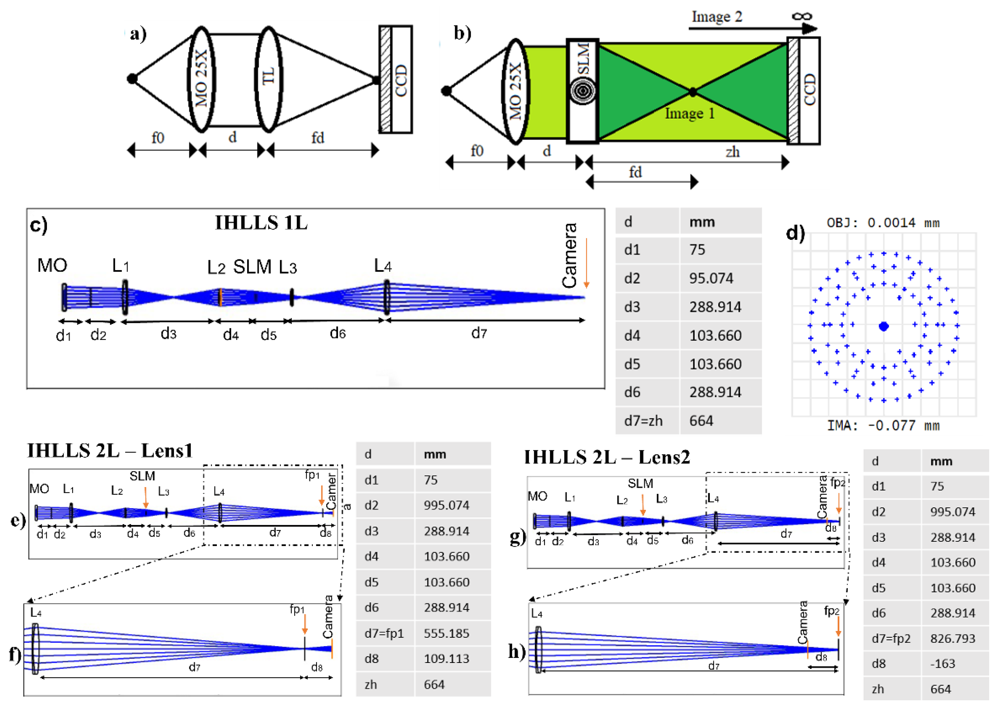
3.1. Fresnel Incoherent Correlation Holography (FINCH) with Dual Lens Adapted for IHLLS

Lattice Light Sheet Microscopy provides a method for the generation of 3D imaging using a self-reinforcing lattice of Bessel beams as an excitation source and imaging the subsequent fluorescence orthogonally. The generation of the lattice light sheet is achieved in multiple steps. The lattice light sheet is formed by projecting a linearly polarized circular laser beam stretched in the x axis with cylindrical lenses and compressed in the z axis onto a spatial light modulator (SLM). A diffraction pattern of the resultant optical lattice using a Fraunhofer lens is directed to a transparent annular mask to eliminate unwanted diffraction orders and lengthen the light sheet. The sheet is dithered to smooth fluctuation in the x plane, and its position is controlled by the z galvanometer (z-axis). In the standard LLS configuration this moves together with the detection objective or with the sample stage for volumetric reconstruction. Both of these methods have disadvantages. Moving the sample prevents combining in situ use of the LLSM with other modalities such as electrophysiology. Moving the objective slows the imaging and generates movement artifacts because of the mass of the objective. The thin illumination depth (~400 nm) of lattice light-sheet microscopy enables high-resolution imaging in the z axis and diffraction limited resolution in the x and y or higher resolutions by creating structured illumination using phase rotations of the Bessel beam lattice. This approach also uses extremely low light doses and little photobleaching. This makes LLS an ideal fluorescence imaging system for many biological studies.
The detection path of the LLS instrument follows a general optical microscopy theory where a plane wave light coming out from an infinity corrected objective passes through a tube lens, which focusses the beam to an image plane at the sensor: Figure 1a (green path), Figure 2b. Substituting the limited tube lens for a versatile component such as SLM will open the 3D capability of the instrument, eliminating the need for scanning and sectioning. The SLM has multiple roles here: (1) to split a parallel beam of light in two spherical beams; (2) to create two different diffractive lenses on the same SLM with randomly distributed pixels by lens multiplexing [29,32]; (3) to change the phase on one of the diffractive lenses by phase-shifting; and (4) to modulate the phase through adjustment of the spatial distribution of the incoming light such as the phase, polarization state, and intensity of the incoming beam in order to get the maximum phase modulation possible.
We perform self-interference holography using an SLM, called FINCH, as a single optical channel to split the incoming incoherent beam from the sample into two spherical beams: Figure 1b. Because the light is originated from the same point source, the two beams can interfere at the recording camera by simply using the coherence property of the two beams. FINCH is a spatially on-axis incoherent interferometer, and hence a phase-shifting technique is employed to record three or four camera images to suppress the twin image and the background or the zero-order image. To achieve the maximum image resolution, the two interfering beams must overlap perfectly at the detector plane. This happens in two ways: by using a constant phase and a diffractive lens with the focal length being equal to half the distance between the SLM and the camera [32,33], Figure 2b (IHLLS 1L), or to modify the constant phase, which has an infinite focal length, to another diffractive lens. In this way, the system is transformed into a double diffractive lens system with two foci points, before and after the CCD, Figure 2e–h (IHLLS 2L).
Our approach is to use the FINCH technique with only one diffractive lens (IHLLS 1L), as in Figure 2c,d to replicate the original LLS detection path for calibration and alignment purposes, but using incoherent holography, and by displaying two diffractive lens patterns with randomly selected pixels on the SLM, as in Figure 2e–h (IHLLS 2L), to obtain depth sectioning and to record sample holograms. It was demonstrated that such a system with two lenses of close focal lengths yields a better hologram in comparison to a single diffractive lens, FINCH [29]. The dual lens FINCH analysis is covered entirely in [33], and here we will detail the steps to adapt and analyze it for the LLS tube lens of focal length fd = 500 mm.
In the original setup of FINCH, there are no optics between the microscope objective and the SLM or between the SLM and the camera. Therefore, the focal lengths of the diffractive lenses coincide with their imaging distances, calculated from the SLM position toward the camera position. The SLM used here was a reflective-phase SLM (Meadowlark) with a chip size of 1920 × 1152 pixels, 9.3 μm/pixel. This has a smaller diameter than the output of the imaging objective; therefore, the beam was adjusted in size by using the two lens pairs, L1, L2 and L3, L4, to fit the SLM chip area. In this case, the focal lengths of the diffractive lenses, fSLM, fd1, and fd2, uploaded on the SLM, are different than their imaging planes, measured from the SLM toward the camera.
The SLM transparency containing the two diffractive lenses has the expression: C 1 Q 1 f d 1   + C 2 exp i θ Q 1 f d 2 , where Q ( b ) = exp [ i π b λ 1 ( x 2 + y 2 ) ] is a quadratic phase function with (x,y) being the space coordinates, θ is the phase shift of the SLM, and C 1 ,   C 2   are constants. When the system works in IHLLS 2L mode, C 1 = 0.5 and C 2 = 0.5 . When f d 1 = (IHLLS 1L), the expression becomes: C 1 + C 2 exp i θ Q 1 f SLM , and C 1 = 0.1 and C 2 = 0.9 . Let us suppose the two waves, created by the diffractive lenses at the SLM, have the general expressions:
U 1 u , v   = A 1 u , v exp   i ϕ 1 u , v
U 2 u , v   = A 2 u , v exp   i ϕ 2 u , v + θ
where u , v are the coordinates of the camera plane, with the assumption that the object is an infinitesimal object point, the intensity of the hologram at the sensor plane taking the following expression:
I H u , v   = A 1 u , v 2 + A 2 u , v 2 + 2 A 1 u , v A 2 u , v cos   ϕ 1 u , v     ϕ 2 u , v     θ
Then, four phase-shifted holograms with phase shifts applied to one of the diffractive lenses of 0, π / 2 , π , 3 π / 2 , are recorded by the camera and superposed using the phase-shifting algorithm to build the complex hologram of the object point at the camera plane:
U u , v   = A u , v   exp i ϕ u , v   =
1 4 ( I H u , v , 0     I H   u , v , π   +   i ( I H u , v , π 2     I H u , v , 3 π 2
where: A u , v is the amplitude of the encrypted image, which is the product of the two amplitudes, A u , v   = A 1 u , v   A 2 u , v , and the encrypted phase:
φ u ,   v   = ϕ 1 u , v     ϕ 2 u , v   = a r c t a n I H u , v , 0     I H u , v , π I H u , v , π 2     I H u , v , 3 π 2
Therefore, the complex amplitude distribution of the object wave at the camera plane has the expression:
A 1 u , v   exp i ϕ u , v   = U u , v / A 2 u , v
The 3D image of the object is retrieved by using the angular spectrum method to reconstruct the complex amplitude of the object wave at any depth within the positive reconstruction distance,   z r , found by the expression:
z r = ± z h f p 1 f p 2 z h f p 2 f p 1
We used the following values for the dual lens FINCH: f p 1 = 555.185   mm , f p 2 = 826.793   mm . The two focal lenses were calculated using OpticStudio (Zemax, LLC) in a multiconfiguration system, as described in our previous work [24]. The distance between the last lens in the system, L4, and the camera was calculated by the optical design software as being z h = 664   mm , and matches the value calculated with the expression z h = 2 f p 1 f p 2 f p 2 + f p 1 . Therefore, using Equation (7), the reconstruction distance is z r 63   mm , (in terms of lens distances) above and below the middle position of the z-galvo scanning range. If we need to reach out to the most extreme parts of objects in the FOV of the camera, the reconstruction distance could increase to 80   mm . This distance corresponds to a z-galvo range of z galvo = ± 40   μ m (in terms of object distances). This displacement is obtained for the LLS diffraction mask positioned on the anulus of outer NA of 0.55 and inner NA of 0.48, which generated a Bessel beam with an FWHM sheet length of 15 µm.

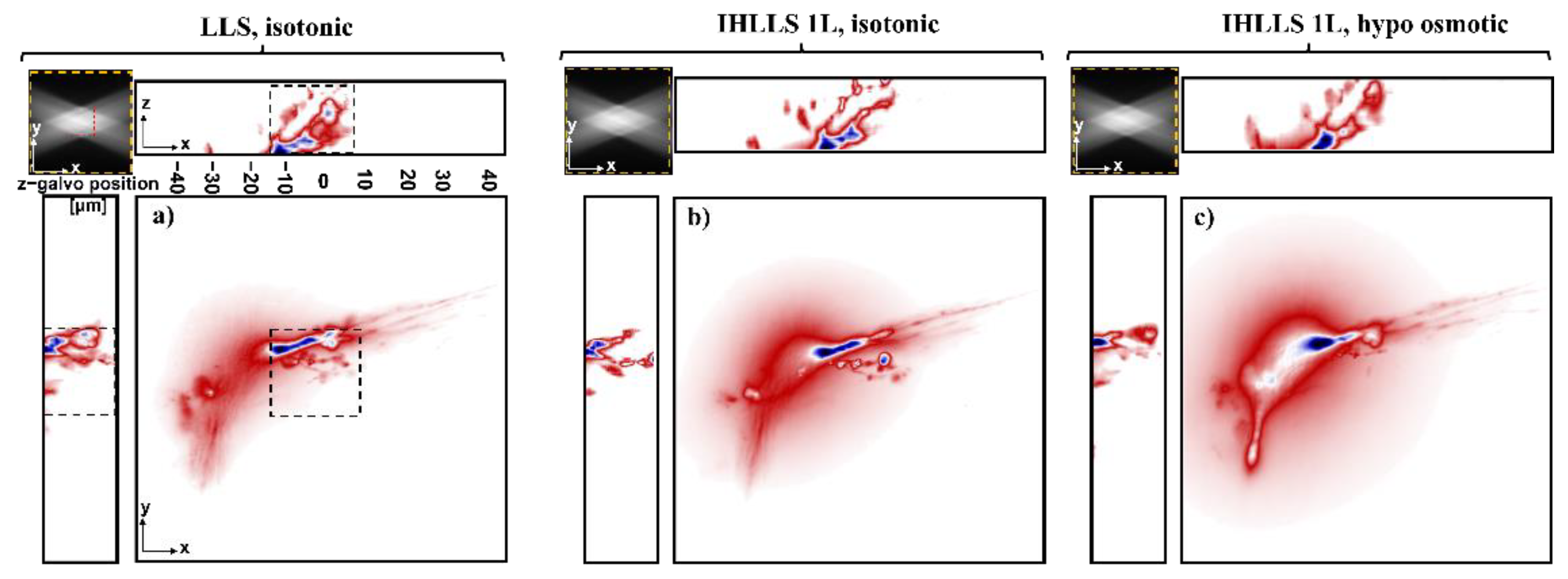
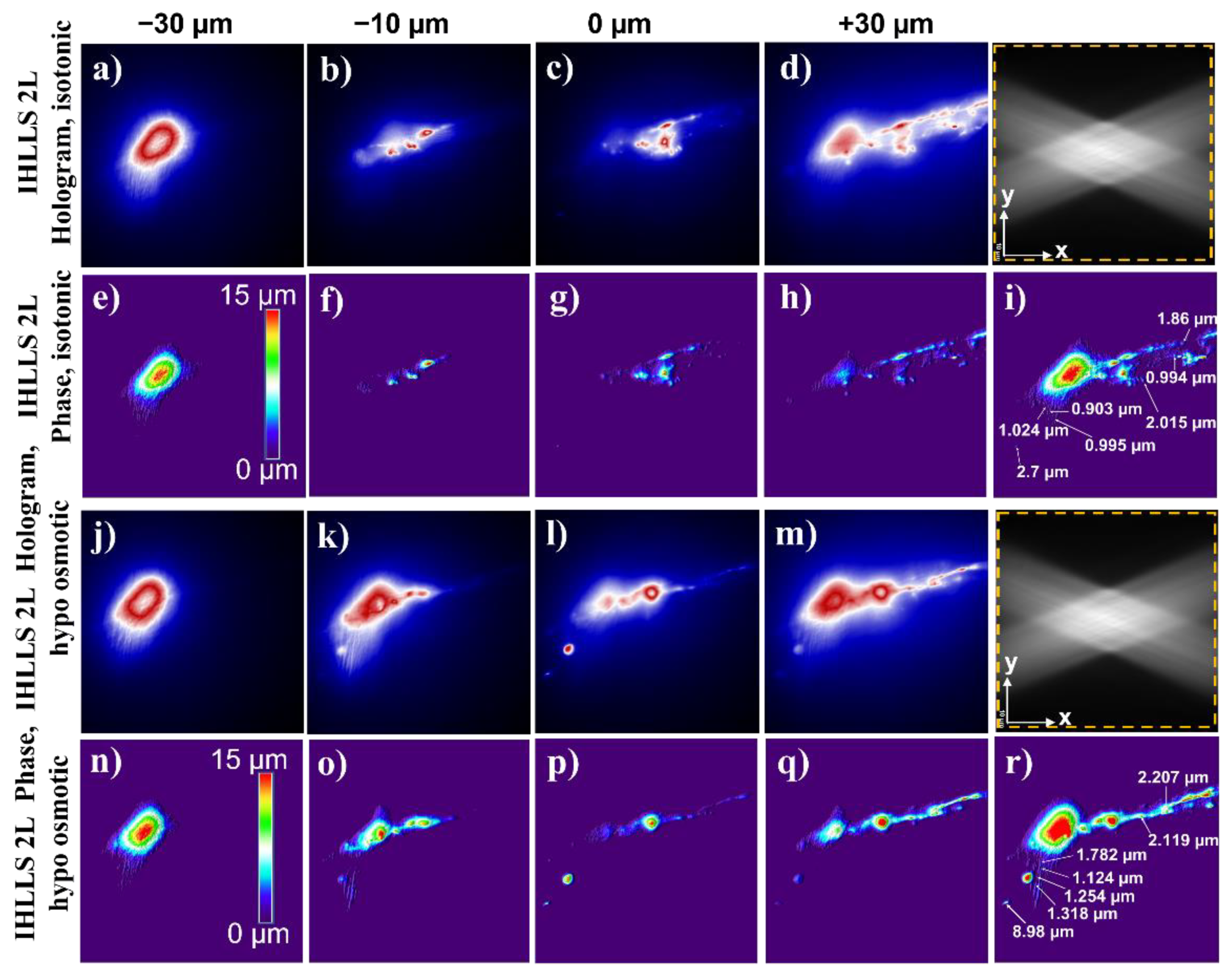
3.2. Imaging Neurons

To examine the effects of applying IHLLS holography, we performed three experiments for this study for calibration purposes. The first was carried out using the conventional LLS pathway, where the z-galvo was stepped in δ z LLS = 0.101   μ m increments through the focal plane of a 25x Nikon objective, which was simultaneously moved the same distance with a z-piezo controller for a displacement range of Δ z galvo = 40   μ m (Figure 3a) for scanning area of 208 × 208   μ m 2 . The second set of images was obtained using the IHLLS 1L with focal length f SLM = 400   mm , displayed on the SLM, where both the z-galvo and z-piezo were again stepped with the same δ z LLS = 0.101   μ m increments through the focal plane of the objective for the same displacement Δ z galvo = 40   μ m . The intensity images using the IHLLS 1L mode were recorded only for the diffractive lens with phase shift θ = 0   . Initially, these images, obtained in both LLS and IHLLS 1L modes, were obtained in isotonic lamprey Ringer’s solution (270 mOsm (Figure 3a,b).
To expand the neurons as an initial test of the ability of the IHLLS system to record small changes in size, we repeated the experiment using the IHLLS 1L, where the Ringer’s solution was modified with hypotonic solution (225 mOsm) (Figure 3c). The third step was achieved by combining the coherent properties of the Bessel beams with the incoherent properties of the fluorescent light emitted by each 3D point of the sample, but made coherent in the self-interference process. This method was performed with both solutions, isotonic and hypotonic solutions, using the IHLLS pathway with two super-imposed diffractive lenses displayed on the SLM comprising randomly selected pixels (IHLLS 2L), where only the z-galvo was moved within the same Δ z galvo = 40   μ m displacement range, above and below the reference focus position of the objective (which corresponds to the middle of the camera FOV), at z galvo = ± 40   μ m   ± 30   μ m , ± 20   μ m ,   ± 10   μ m , and 0   μ m . The two wavefronts interfere with each other at the camera plane to create Fresnel holograms. Four interference patterns were created using a phase shifting technique ( θ = 0 ,   θ = π / 2 , θ = π , θ = 3 π / 2 ) and further combined mathematically to obtain the complex amplitude of the object point at the camera plane. The results are summarized in Figure 4, which depicts the samples in isotonic (Figure 4a–i) or hypotonic solutions (Figure 4j–r), at four z-galvo planes, denoted z galvo = ± 30   μ m , 10   μ m , and 0   μ m . The z-galvo planes correspond to the same relative depths in the sample. Four holographic images were recorded for each z-galvo position and combined mathematically to build the complex amplitude of each sample. The 3D field was reconstructed at various depth positions, and those images in focus at certain planes were chosen to build the tomographic structure of the neuronal cell. We performed scanning at nine z-galvo positions and, therefore, nine phase images were selected to build the tomographic slice of all nine superposed images (Figure 4i,r). It is clear from this that the soma (Figure 4e compared to Figure 4n) and the dendrites (Figure 4f–h compared to Figure 4o–q) all showed an increase in volume. We have emphasized this by measuring the phase values of various points in the neuron’s dendritic tree and calculating the optical path length that this represents, first in isotonic solution and then in hypo-osmotic solution. This treatment is expected to swell the neurons, including the dendritic tree, increasing the size of these structures. The analyses indicate that the technique can resolve sub-micrometer size changes, represented in depth by the color coding shown in Figure 4. For comparison, we measured the diameters of well separated structures in the xy plane, which are expected to be similar to the depth in these cylindrical structures. We have inserted these numbers in Figure 4i,r. The diameters measured increased from 1.41 ± 0.50 to 2.28 ± 1.04 µm. These are also clearly resolvable from the depth encoding.

4. Discussion

In a prior study [24], we demonstrated the capacity of the IHLLS system to reconstruct 3D positions of beads as light point sources using a very reduced number of z-galvo mirror scanning planes when compared to the original LLS system using the dithered mode. We also showed the same or slightly improved resolution of the bead positions. The IHLLS system can therefore provide faster volumetric image acquisition and multi-plane imaging for probing the three-dimensional morphology and structure of biological samples.
The use of IHLLS enhances lattice light sheet microscopy in several ways. In LLS, focus of the emission objective must be maintained in the focal plane of the lattice sheet, requiring movement of a bulky objective, which takes time, but also, at the high speeds of LLS imaging, will apply fluid pressure movements across the sample. This will potentially distort images, but in addition will provide noise to transient measurements of cell surfaces caused by rapid activity, for example, action potential firing in excitable cells. It is also difficult to resolve very small changes in surface structure at speed, even with volumetric imaging. Consequently, the ability to resolve rapid surface structure changes, without moving the objective lens, and higher accuracies than traditional volumetric imaging approaches is valuable. In this study, we have demonstrated that IHLLS can be used to resolve artificially applied changes in neuron shape. We will seek in further studies to relate these changes to physiological activity.
Although we eliminated the z-piezo objective motion needed to maintain the object focus, there are a few challenges in approaching this work. The conventional LLS system uses a very low dose of light and low exposure time without a polarizer in the detection path. The digital incoherent holography technique with two diffractive lenses uses two polarizers in the detection arm; therefore, the light dose and the exposure time has to be increased from the middle of the z-galvo scanning range toward the two ends of the scanning range to maintain a similar signal efficiency to the conventional LLS, but low enough to preserve the biological samples. For this reason, we opted to use a double diffractive lens FINCH technique with randomly selected pixels, which requires only one polarizer mounted before the SLM to align the input beam to its active axis. The SLM was also positioned at 11° deflection angle to generate active beam steering at the highest efficiency. Another challenge in this configuration is the beam size of 17.6 mm in the back focal plane of the microscope objective (Nikon, CFI Apo LWD 25XW, 1.1 NA, 2 mm WD, Tokyo, Japan), which is too large for the SLM chip size (17.66 mm × 10.6 mm, Meadowlark Optics Inc., Longmont, CO, USA), and we decided to place the SLM in a double 4f optic system configuration made by two lenses with a 200 mm focal length and two lenses with a 125 mm focal length. This combination has also helped to decrease the z h min to about 664 mm.

Author Contributions

Conceptualization, M.P. and S.A.; methodology, M.P. and S.A.; software, M.P. and C.M.; validation, M.P., S.A., J.A. and C.M.; resources, S.A., J.A. and C.M.; data curation, M.P., S.A. and C.M.; writing—original draft preparation, M.P. and S.A.; writing—review and editing, M.P., S.A., J.A. and C.M.; visualization, M.P., S.A., J.A. and C.M.; supervision, S.A. and J.A.; project administration, S.A. and J.A.; funding acquisition, S.A. and J.A. All authors have read and agreed to the published version of the manuscript.

Funding

This research was funded by the NIH RO1 NS111749 to S.A. and the NIH R21 DC017292 to J.A., and the National Institutes of Health (123456) and National Science Foundation (456789) to C.M.

Institutional Review Board Statement

All work on animals was performed according to Institutionalization guidelines in an AALAC approved facility. Date of last institutional approval 8 March 2018. The work was approved by the institutional IACUC review committee under protocol number ACC 20-119 on 16 April 2021.

Data Availability Statement

Supporting data for Figure 3 and Figure 4 are available from the corresponding author on reasonable request. This is due to the size of the datasets being so large that they are not available on a public server.

Conflicts of Interest

The authors declare no conflict of interest.

References

  1. Julius, D.; Nathans, J. Signaling by sensory receptors. Cold Spring Harb. Perspect. Biol. 2012, 4, a005991. [Google Scholar] [CrossRef] [Green Version]
  2. Bader, D.L.; Knight, M.M. Biomechanical analysis of structural deformation in living cells. Med Biol. Eng. Comput. 2008, 46, 951–963. [Google Scholar] [CrossRef] [PubMed] [Green Version]
  3. Lankford, C.K.; Laird, J.G.; Inamdar, S.M.; Baker, S.A. A Comparison of the Primary Sensory Neurons Used in Olfaction and Vision. Front. Cell. Neurosci. 2020, 14, 595523. [Google Scholar] [CrossRef] [PubMed]
  4. Hodgkin, A.L.; Huxley, A.F. A Quantitative Description of Membrane Current and Its Application to Conduction and Excitation in Nerve. J. Physiol. 1952, 117, 500–544. [Google Scholar] [CrossRef] [PubMed]
  5. Knöpfel, T.; Tomita, K.; Shimazaki, R.; Sakai, R. Optical recordings of membrane potential using genetically targeted voltage-sensitive fluorescent proteins. Methods 2003, 30, 42–48. [Google Scholar] [CrossRef]
  6. Fillafer, C.; Mussel, M.; Muchowski, J.; Schneider, M.F. Cell Surface Deformation during an Action Potential. Biophys. J. 2018, 114, 410–418. [Google Scholar] [CrossRef] [Green Version]
  7. Mueller, J.K.; Tyler, W.J. A quantitative overview of biophysical forces impinging on neural function. Phys. Biol. 2014, 11, 051001. [Google Scholar] [CrossRef] [Green Version]
  8. Zhang, P.-C.; Keleshian, A.M.; Sachs, F. Voltage-induced membrane movement. Nature 2001, 413, 428–432. [Google Scholar] [CrossRef]
  9. Lindau, M.; Neher, E. Patch-clamp techniques for time-resolved capacitance measurements in single cells. Pflügers Arch. 1988, 411, 137–146. [Google Scholar] [CrossRef] [PubMed]
  10. Sankaran, J.; Wohland, T. Fluorescence strategies for mapping cell membrane dynamics and structures. APL Bioeng. 2020, 4, 020901. [Google Scholar] [CrossRef]
  11. Boulanger, J.; Gueudry, C.; Münch, D.; Cinquin, B.; Paul-Gilloteaux, P.; Bardin, S.; Guérin, C.; Senger, F.; Blanchoin, L.; Salamero, J. Fast high-resolution 3D total internal reflection fluorescence microscopy by incidence angle scanning and azimuthal averaging. Proc. Natl. Acad. Sci. USA 2014, 111, 17164–17169. [Google Scholar] [CrossRef] [Green Version]
  12. Tolde, O.; Gandalovičová, A.; Křížová, A.; Veselý, P.; Chmelík, R.; Rosel, D.; Brábek, J. Quantitative phase imaging unravels new insight into dynamics of mesenchymal and amoeboid cancer cell invasion. Sci. Rep. 2018, 8, 1–13. [Google Scholar] [CrossRef] [Green Version]
  13. Lu, T.; Anvari, B. Characterization of the Viscoelastic Properties of Ovarian Cancer Cells Membranes by Optical Tweezers and Quantitative Phase Imaging. Front. Phys. 2020, 8. [Google Scholar] [CrossRef]
  14. Jaferzadeh, K.; Sim, M.; Kim, N.; Moon, I. Quantitative analysis of three-dimensional morphology and membrane dynamics of red blood cells during temperature elevation. Sci. Rep. 2019, 9, 1–9. [Google Scholar] [CrossRef] [PubMed] [Green Version]
  15. Jaferzadeh, K.; Moon, I.; Bardyn, M.; Prudent, M.; Tissot, J.-D.; Rappaz, B.; Javidi, B.; Turcatti, G.; Marquet, P. Quantification of stored red blood cell fluctuations by time-lapse holographic cell imaging. Biomed. Opt. Express 2018, 9, 4714–4729. [Google Scholar] [CrossRef]
  16. Rappaz, B.; Barbul, A.; Hoffmann, A.; Boss, D.; Korenstein, R.; Depeursinge, C.; Magistretti, P.J.; Marquet, P. Spatial analysis of erythrocyte membrane fluctuations by digital holographic microscopy. Blood Cells Mol. Dis. 2009, 42, 228–232. [Google Scholar] [CrossRef] [PubMed]
  17. Yu, L.; Mohanty, S.; Zhang, J.; Genc, S.; Kim, M.K.; Berns, M.; Chen, Z. Digital holographic microscopy for quantitative cell dynamic evaluation during laser microsurgery. Opt. Express 2009, 17, 12031–12038. [Google Scholar] [CrossRef] [Green Version]
  18. Gabor, D. A New Microscopic Principle. Nature 1948, 161, 777–778. [Google Scholar] [CrossRef] [PubMed]
  19. Mann, C.J.; Yu, L.; Lo, C.-M.; Kim, M.K. High-resolution quantitative phase-contrast microscopy by digital holography. Opt. Express 2005, 13, 8693–8698. [Google Scholar] [CrossRef] [PubMed] [Green Version]
  20. Khmaladze, A.; Kim, M.; Lo, C.M. Phase imaging of cells by simultaneous dual-wavelength reflection digital holography. Opt. Express 2008, 16, 10900–10911. [Google Scholar] [CrossRef] [PubMed]
  21. Kim, M.K. Principles and techniques of digital holographic microscopy. J. Photon. Energy 2010, 1, 018005. [Google Scholar] [CrossRef] [Green Version]
  22. Ferraro, P. Coherent Light Microscopy: Imaging and Quantitative Phase Analysis; Ferraro, P., Wax, A., Zalevsky, Z., Eds.; Springer: Berlin/Heidelberg, Germany, 2011. [Google Scholar]
  23. Rosen, J.; Kelner, R. Modified Lagrange invariants and their role in determining transverse and axial imaging resolutions of self-interference incoherent holographic systems. Opt. Express 2014, 22, 29048–29066. [Google Scholar] [CrossRef] [PubMed] [Green Version]
  24. Potcoava, M.; Mann, C.; Art, J.; Alford, S. Spatio-temporal performance enhancement in an incoherent holography lattice light-sheet microscope (IHLLS). Opt. Express 2021, 29, 23888–23901. [Google Scholar] [CrossRef]
  25. Gao, L.; Shao, L.; Chen, B.-C.; Betzig, E. 3D live fluorescence imaging of cellular dynamics using Bessel beam plane illumination microscopy. Nat. Protoc. 2014, 9, 1083–1101. [Google Scholar] [CrossRef]
  26. Chen, B.C.; Legant, W.R.; Wang, K.; Shao, L.; Milkie, D.E.; Davidson, M.W.; Janetopoulos, C.; Wu, X.S.; Hammer, J.A.; Liu, Z.; et al. Lattice light-sheet microscopy: Imaging molecules to embryos at high spatiotemporal resolution. Science 2014, 346, 1257998. [Google Scholar] [CrossRef] [Green Version]
  27. Rosen, J.; Brooker, G. Digital spatially incoherent Fresnel holography. Opt. Lett. 2007, 32, 912–914. [Google Scholar] [CrossRef]
  28. Rosen, J.; Brooker, G. Non-scanning motionless fluorescence three-dimensional holographic microscopy. Nat. Photon. 2008, 2, 190–195. [Google Scholar] [CrossRef]
  29. Katz, B.; Rosen, J.; Kelner, R.; Brooker, G. Enhanced resolution and throughput of Fresnel incoherent correlation holography (FINCH) using dual diffractive lenses on a spatial light modulator (SLM). Opt. Express 2012, 20, 9109–9121. [Google Scholar] [CrossRef] [PubMed] [Green Version]
  30. Brooker, G.; Siegel, N.; Wang, V.; Rosen, J. Optimal resolution in Fresnel incoherent correlation holographic fluorescence microscopy. Opt. Express 2011, 19, 5047–5062. [Google Scholar] [CrossRef] [Green Version]
  31. Bouchal, P.; Bouchal, Z. Wide-field common-path incoherent correlation microscopy with a perfect overlapping of interfering beams. J. Eur. Opt. Soc. Rapid Publ. 2013, 8, 13011. [Google Scholar] [CrossRef] [Green Version]
  32. Rosen, J.; Siegel, N.; Brooker, G. Theoretical and experimental demonstration of resolution beyond the Rayleigh limit by FINCH fluorescence microscopic imaging. Opt. Express 2011, 19, 26249–26268. [Google Scholar] [CrossRef] [PubMed]
  33. Rosen, J.; Brooken, G. Fresnel incoherent correlation holography (FINCH): A review of research. Adv. Opt. Technol. 2012, 1, 151–169. [Google Scholar] [CrossRef]
Figure 1. The detection modules of (a) the commercial LLS microscope, LLS (red), and incoherent holographic detection module, IHLLS (green). (b) The optical setup of the IHLLS detection module. The system consists of a water immersed microscope objective MO (Nikon 25X, NA 1.1, WD 2 mm), lenses L1 = L4 with focal lengths 175 mm, L2 = L3 with focal lengths 100 mm; mirrors M1, M2, M3; polarizer P; 520 nm center wavelength, band pass filter BPF with bandwidth Δ λ = 40   nm ; and spatial light modulator SLM. The light propagates through either pathway 1 (red line in a), for the original LLS, or pathway 2 (green line in a) for IHLLS, depending on the orientation of sliding mirror.
Photonics 08 00383 g001
Figure 2. Optical setup terminology of LLS and IHLLS: (a) Schematic of the LLS detection path, MO: microscope objective of 25X with NA 1.1 and f0 = 8 mm, TL: tube lens of focal length fd = 500 mm that focusses on the camera; (b) FINCH schematic with only one diffractive lens of focal length fd, and a phase constant (spherical wave with infinite radius) applied on the SLM, zh is the distance between the SLM and camera, zh = 2fd for the best overlap of the two beams at camera; (c) Ray tracing using only one diffractive lens in IHLLS 1L, with a focal length of fSLM = 400 mm. The focal length was calculated using OpticStudio (Zemax, LLC), with the constraint used for the optimization process that the transversal magnification of the two systems, LLS and IHLLS-1L, should be the same: M T IHLLS   1 L = M T LLS = 62.5 ; (d) The spot diagram from (c); (e) Ray tracing using two diffractive lenses, IHLLS 2L, of focal lengths fd1 = 220 mm and fd2 = 2356 mm, and fp1 being the first imaging position at 109 mm in front of the camera; (f) The inset shows that the first imaging position is placed in front of the camera; (g) Ray tracing using two diffractive lenses, IHLLS 2L, with fp2 being the second imaging position at 163 mm behind the camera; (h) The inset shows that the first imaging position is placed in front of the camera. The two focal distances, fd1 and fd2, were obtained from a multi-configuration optical system with the condition that the height of the two beams was equal at the camera plane for a perfect overlap; distance d1 is the distance between the MO and a dummy surface with infinite radius needed to check the beam collimation after the MO. Distance d2 is the distance between the dummy surface and lens L1. Lenses L1 = L4 with focal lengths 175 mm and L2 = L3 with focal lengths 100 mm.
Photonics 08 00383 g002
Figure 3. Tomographic imaging of a lamprey spinal cord ventral horn neuron with dendrites, xy FOV 208 × 208 µm2, 2048 × 2048 pixels, yz, (xz) FOV 208 × 40 µm2, 2048 × 400 pixels, in a conventional LLS (a) and incoherent LLS with only one diffractive lens (IHLLS 1L) of focal length 400 mm without deconvolution; recordings were initially in isotonic solution (b), and then in hypotonic solution to cause swelling (c). On the sides and above are shown the max projections through the volume (400 z-galvo steps). The Bessel beams are displayed in the upper-left corner of each xy-projection to show the orientation of the beams (FOV 208 µm2). The area enclosed inside the colored dashed rectangles are as follows: black—the scanning area for the original LLS (52 µm2), and yellow—the actual scanning area for the LLS, IHLLS 1L, and IHLLS 2L.
Photonics 08 00383 g003
Figure 4. IHLLS 2L imaging of a lamprey spinal cord ventral horn neuron with dendrites in a Ringer’s solution (ai) and hypotonic solution (jr), FOV 208 × 208 µm2, 2048 × 2048 pixels; (ad,jm) imaging holography at 30   μ m , 10   μ m , 0   μ m , and + 30   μ m , for the phase-shift θ = 0; (eh,nq) the corresponding reconstructed phase images; (i,r) the superposition of all reconstructed phase images at ± 40   μ m , ± 30   μ m ,   ± 20   μ m , ± 10   μ m ,   and   0   μ m . The Bessel beams are displayed in the right gray panel of each xy-projection to show the orientation of the beams (FOV 208 × 208 µm2). The phase values of the reconstructed images were converted to the optical path length values in reflection mode.
Photonics 08 00383 g004
Publisher’s Note: MDPI stays neutral with regard to jurisdictional claims in published maps and institutional affiliations.

