Using Machine Learning Algorithms for Accurate Received Optical Power Prediction of an FSO Link over a Maritime Environment

Abstract

The performance prediction of an optical communications link over maritime environments has been extensively researched over the last two decades. The various atmospheric phenomena and turbulence effects have been thoroughly explored, and long-term measurements have allowed for the construction of simple empirical models. The aim of this work is to demonstrate the prediction accuracy of various machine learning (ML) algorithms for a free-space optical communication (FSO) link performance, with respect to real time, non-linear atmospheric conditions. A large data set of received signal strength indicators (RSSI) for a laser communications link has been collected and analyzed against seven local atmospheric parameters (i.e., wind speed, pressure, temperature, humidity, dew point, solar flux and air-sea temperature difference). The k-nearest-neighbors (KNN), tree-based methods-decision trees, random forest and gradient boosting- and artificial neural networks (ANN) have been employed and compared among each other using the root mean square error (RMSE) and the coefficient of determination (R²) of each model as the primary performance indices. The regression analysis revealed an excellent fit for all ML models, indicative of their ability to offer a significant improvement in FSO performance modeling as compared to traditional regression models. The best-performing R² model found to be the ANN approach (0.94867), while random forests achieved the most optimal RMSE result (7.37).

1. Introduction

Free-space optical communication (FSO) technology has been around for a long time. Perhaps the first kind of FSO system was the photophone that Alexander Graham Bell invented in 1880. Since then, FSO technology has progressed through extensive research efforts, and has even reached NASA’s and ESA’s deep-space communications projects [1]. FSO communication is based on data transmission in unguided propagation media through the use of optical carriers in the vicinity of the visible to near-infrared (NIR) spectrum. This fact allows for a much higher optical bandwidth comparing to their radio-frequency (RF) counterparts, thus providing an excellent solution for high rate communication within a range of several kilometers [2]. A wide variety of applications can be suitable for FSO communications, ranging from inter-chip connection to inter-satellite communication [2]. The main attractive features of FSO communications can be summarized to (i) the smaller size, weight and power (SWaP) requirements, (ii) the high-gain concentrated energy delivered due to the laser narrow beam and (iii) the absence of any license restrictions due to their operational wavelength [3]. In order to assess the performance of an FSO link, we usually make use of the ratio between the signal power received and the signal power required to achieve a specified data rate with certain error probability, namely the “link margin” [4]. Therefore, given a specified sensitivity threshold for an FSO system, we can assess its performance by measuring the received signal strength indicators (RSSI) in a certain location under different conditions. The RSSI parameter plays a key role to the functional behavior of a hybrid RF/FSO, since it determines the switch from one mode to another.

Apparently, the FSO technology does not come without limitations for its performance. Since the optical signal travels through the atmosphere, it experiences losses due to several factors. The major cause of performance loss is molecular and aerosol absorption and scattering of the propagating beam. In order to quantify this attenuation, the optical depth (τ) that relates the transmitted to received power is utilized as a suitable metric, and their ratio determines the atmospheric transmittance [5]. Several atmospheric “windows” exist where absorption effect is minimized, which is where most FSO systems operate. Moreover, the scattering effect is strongly related to the relative size of the particles to the optical signal wavelength and causes signal energy to be re-distributed in random directions. Secondary, but not negligible, losses are caused due to free-space propagation, divergence of the beam, weather conditions effects and pointing errors. All previously mentioned effects result in received power degradation that, in the worst-case scenario, can even cause link outages and increased bit error rate (BER), thus directly affecting the system’s performance and reducing the effective operational range of the link [6]. Another significant limiting factor is the atmospheric turbulence, characterized by the random fluctuations of the refractive index (n) due to pressure and temperature variations along the beam path. Turbulence gives rise to intensity fluctuations of the received signal, the so-called scintillation effect, which in turn causes a loss of SNR and induces signal fades [5].

The characterization of the refractive index structure parameter within the surface layer has been a long lasting independent research effort for different kinds of surfaces and atmospheric conditions. Over the past 20 years, the US Naval Research Laboratory (NRL) has conducted extensive atmospheric turbulence measurements, focusing on the maritime environment. Their main goal has been atmospheric propagation research and photonic components development in order to characterize and overcome the limitations due to turbulence effects. In doing so, NRL has developed a maritime lasercomm test facility (LCTF), consisting of facilities 16-km apart on both sides of Chesapeake Bay, equipped with instruments to measure transmission, the scintillation index and angle of arrival of the beam [7,8,9,10,11,12,13]. During another trial (FATMOSE), high resolution images were collected by point sources at a range of 15.7 km, along with turbulence related atmospheric parameters that provided statistical information on the mean and variance of the atmospheric point spread function and the associated modulation transfer function during a series of consecutive frames [14]. An experimental set-up to control and measure the effect of laser beam broadening due to turbulence has been designed [15]. In [16], a weather research and forecasting (WRF) model was used to calculate routine meteorological parameters and the refractive index structure parameter near the ocean surface using Monin-Obukhov similarity theory. In [17], this work has been extended to estimate surface layer C_n² over snow and ice and gave even better results than estimations over the ocean. In [18], an approach was developed to quantify scintillation by estimating the refractive index structure parameter from surface fluxes that are derived from single-level routine weather data. Frehich et al. related the structure functions of the atmospheric variables with spatial structure functions of the numerical weather prediction (NWP) model variables [19].

Atmospheric turbulence and environmental conditions have directly negative effects on an FSO link’s performance in terms of its reliability and even its availability. Extensive experimental and theoretical research has been conducted for various communication schemes and performance metrics, both for terrestrial and maritime environments. Bourazani et al., have studied the weak gamma-distributed turbulence effects on the bit rate of an FSO link over sea [20]. A theoretical work in [21] examined the atmospheric turbulence induced fading modeled by the M-distribution and the line-of-sight (LOS) blockage of an FSO link. Kong et al. investigated the average symbol error rate (ASEP) of a hybrid RF/FSO link [22]. Alheadary et al. reported on the modelling of the channel attenuation coefficient for a coastal environment, taking into consideration the air temperature, humidity and dew point by employing an FSO system with 70 m link length [23]. In [24], the signal fluctuations due to atmospheric turbulence and extinction effects was measured in terms of RSSI, using a commercial FSO communication system. The same performance metric (i.e., RSSI) was used in [25] in conjunction with several real-time measured atmospheric properties and resulted in two empirical equations for day and night. Lionis et al. simulated the atmospheric effects of a laser beam propagating from an airborne high-speed moving platform, showing that the turbulence effect in a downward slant path is less severe [26]. In [27,28], a second-order polynomial model is constructed to predict RSSI values for a maritime FSO link based on real-time macroscopic meteorological parameters, and different standard probability distributions were evaluated against the RSSI distribution.

This work provides a comprehensive study for the performance prediction of a commercial FSO link over a maritime environment. A large data set of seven macroscopic meteorological parameters, acquired over a period of 12 months, is utilized to predict the received signal strength (i.e., RSSI) by employing regression model analysis. The variance selection of these seven parameters was chosen based on the knowledge that they can strongly affect FSO performance [27,28]. In doing so, five machine learning algorithms are employed, including the KNN, decision trees (DT), gradient boosting regression (GBR), random forest (RF) and ANN. An 80% of the input data set is used to train each model, whereas the remaining 20% is used to evaluate the fitting accuracy, using the RMSE and the R² parameter as the performance metrics. The respective percentage of each subset for the ANN model is 70%, 15% and 15%, due to a validation subset added to fine-tune the trained model hyperparameters. The analysis resulted in an excellent fit for all the algorithms (R² > 0.85). The relative importance of each meteorological parameter for RSSI prediction is also extracted, showing that ambient temperature is the most important.

The remainder of this work is organized as follows: Section 2 provides the background for the statistical learning and the experimental set-up for the data collection, Section 3 presents the results of the regression analysis using ML algorithms and Section 4 concludes the paper.

2. Materials and Methods

Machine learning for optical communications is an emerging topic that will certainly gain more interest in the near future. Machine learning includes a broad spectrum of tools that allows for the interpretation and understanding of data through a trained algorithm. Broadly speaking, there are two main types of ML algorithms: supervised and unsupervised. Supervised learning algorithms are trained using labeled examples, such as an input where the output is known. On the other hand, unsupervised algorithms do not assume a known output for a set of input values [29]. Input variables -or predictors- are denoted with an X whereas the output variable or response is denoted with a Y. Usually, the predictors are more than one and it is assumed that a general relationship among them exists,

$$Y=f(X)+\epsilon$$

(1)

where f is an unknown function and ε is a zero mean random error, statistically independent of X. Supervised learning is focused on estimating this function f for prediction and inference purposes. Having estimated f, one can predict the output for a specific set of input variables. The accuracy of this prediction depends upon the so-called reducible and irreducible errors. The reducible error refers to the inherent inaccuracy due to any inappropriateness of the function f, whereas the irreducible error is included otherwise, since Y is a function of ε. On the other hand, inference refers to the understanding of the relationship between inputs and outputs and the impact of certain changes in inputs on their corresponding output [29]. Problems with a quantitative response are called regression problems, whereas problems with a qualitative response are called classification problems. The various ML algorithms are also categorized as parametric or non-parametric. A parametric model assumes a specific form or shape for the function f, such as a linear or polynomial regression model. A non-parametric, on the other hand, does not make any assumptions about f; rather, it tries to estimate its form based on the training data points [29]. This paper is focused on supervised learning methods for regression models.

2.1. Assessing Model Accuracy

In order to estimate the function f that best fits a data set, we have to be aware of the special attributes it possesses in terms of accuracy and interpretability. For example, a linear regression algorithm may be very clear to interpret but also very restrictive, especially when a non-linear relationship between input and output actually holds. On the other hand, algorithms such as support vector machines or boosting methods could lead to such complicated models that may be very difficult to interpret [29]. However, if prediction accuracy is the desired outcome, models with high flexibility seem to be the best choice. This is not always the case though, since overfitting of the data will, despite decreasing the training error, increase the testing error. Therefore, a careful bias-variance tradeoff has to take place before selecting the most appropriate model. The term variance refers to how much f will change if the same model is used on a different data set, whereas bias refers to the error introduced by modeling a real-life problem. In general, more flexible models tend to increase the variance and decrease the bias [29].

2.2. Machine Learning Based FSO Research Background

An important challenge in using machine learning techniques for scientific applications is to be able to use domain knowledge and data-driven algorithms in synergy. Machine learning algorithms have already been exploited by the optical communications community and, in particular, the free space optical communications community. For example, in [30], a data-driven fiber channel deep learning (DL) modeling method was introduced in an optical communication system. Specifically, a bidirectional long short-term memory was selected to perform fiber channel modeling for on-off keying (OOK) and pulse amplitude modulation 4 signals. A deep learning based atmospheric turbulence compensation method to correct the distorted vortex beam and improve the performance of orbit angular momentum (OAM) multiplexing communication is presented in [31]. FSO related channel modeling is studied using DL techniques in [32] for all turbulence strength regimes, and results published therein indicate that DL can provide performance that is reasonably close to the perfect channel estimation scheme. The ability to mitigate the negative effects of atmospheric turbulence for FSO systems performance is studied in [33,34,35] using ANN, generative machine learning (GML) and convolutional neural networks (CNN) through simulated and experimentally obtained data. ML techniques using DT, RF and ANN for C_n² estimation, is presented in [36,37] and compared against macroscopic meteorological parameters. Other ML algorithms have also been used to predict RSSI for a hybrid RF/FSO detector by developing both regression and classification models [38,39]. Finally, an overview of the, as expected, next generation of the ANN, the so-called optical neural networks (ONNs) and previous studies on the field are reviewed in [40]. The novelty of the current study lies in the comparison of various classical ML algorithms that are presented for the first time in predicting RSSI measurements, especially for the particular domain of interest, Piraeus, Greece. The contribution of this paper is that it a) provides an extension of previous related works in terms of the utilized ML algorithms (i.e., KNN and ANN), which both performed sufficiently enough and b) provides a unique experimental data analysis in terms of the terrain of the link (i.e., maritime), which exhibits different characteristics from a terrestrial one.

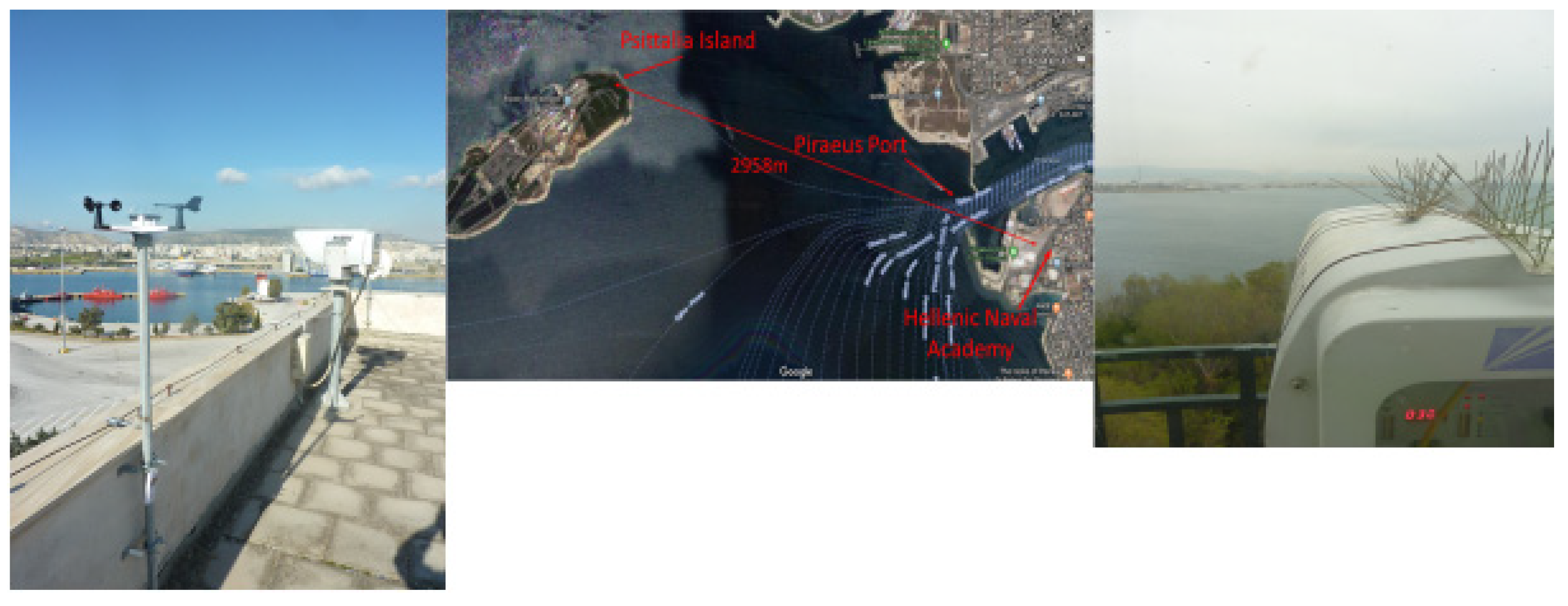
2.3. Measurement Systems Overview

In order to measure the received signal strength for a real FSO system, a 2958-m propagation path was established over Piraeus port entrance at the Hellenic Naval Academy (HNA), Piraeus, Greece. A commercial FSO system was used to take RSSI measurements, to compare with the model predictions. Specifically, the FSO system used in the experiments is a MRV TS500/155 transceiver, operating at 850 nm with a maximum output power of 150-mW and data rate of 155-Mbps. It utilizes three laser sources with a beam divergence of 2 mrad each and a single receiver with a diameter of 20-cm, a sensitivity of −46 dBm and an avalanche photodetector (APD). It also uses an open protocol to automatically identify and lock on the current data rate and clock. The first terminal was located on the roof of a building at HNA, whereas the second was located on the Psytalia Island lighthouse. The horizontal propagation path was approximately 35 m above the surface of the sea, and over 95% of it was over water. Tidal changes in that area are minimal; therefore altitude changes of the propagation path were ignored. A diagram of the MRV, WS-2000 weather station and the surrounding area are shown in Figure 1. In addition to collecting measured readings from the FSO system, a WS-2000 weather station near the MRV was deployed to measure macroscopic meteorological parameters, including ambient temperature, air pressure, relative and absolute humidity, dew point, solar flux, ultra-violet index, rainfall rate, wind speed and direction. An online weather statistics database, [41] was also exploited to take sea temperature measurements from which the air-sea temperature difference was estimated. Measurements from both sensors were taken every minute, twenty-four hours per day.

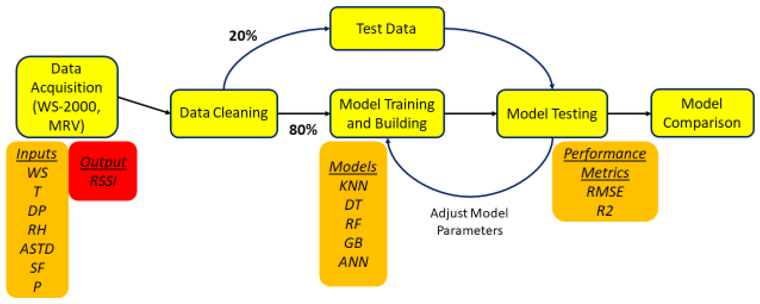
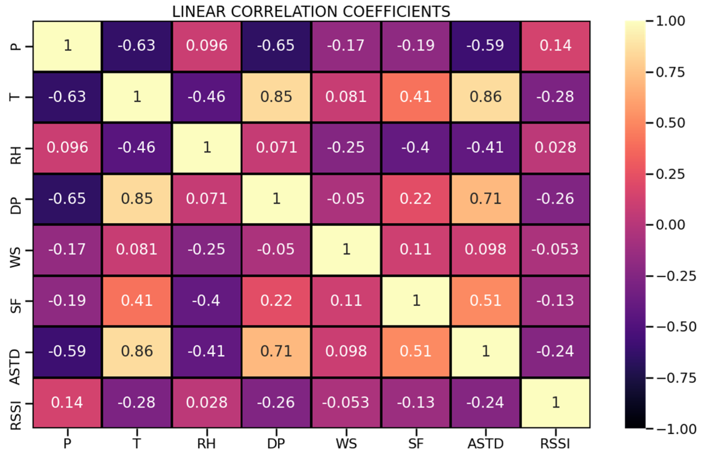
2.4. Methodology of Analysis

The findings of this paper are based on a large data set of measurements recorded between the 30 November 2019 and the 27 October 2020. Several technical issues, including system resets and line-of-sight blockages due to maritime traffic, did not allow for continuous measurements. Additional data cleaning before analysis reduced the data points to a total amount of 144,803. Both sensors internal clocks were synchronized and the measurements were taken at one-minute intervals. The input data obtained from the WS-2000 station into a xlsx file format. Data were screened, and redundant recorded data were excluded to settle on a clean dataset of eight columns, including wind speed in m/s, air temperature in K degrees, dew point in °C, relative humidity (%), air-sea temperature difference in °C, solar flux in W⋅m⁻² and relative pressure in mbar. An additional column was added to include the water temperature from the online database. Each data row was then compounded with the respective output value of RSSI for the same date/time. Therefore, a single user-friendly file was compiled for further process and analysis. Any measurements with missing or non-physical values were excluded. For example, the heavy maritime vessel traffic entering or leaving the Piraeus port caused many of the RSSI values to not be accurate. After collecting, compiling and cleaning the data set, the machine learning process was initiated. The first step was to take the set of all observations and divide it randomly into two subsets. The first subset was used to train the model. The second subset was used to test the model once it had been trained. This second dataset is referred to as the test subset. The objective is to estimate the performance of the machine-learning model on new data (i.e., data not used to train the model). There is not an optimal percentage in which to split the data set; rather, it is required to account for the computational cost to train and test the model as well as an adequate representativeness in the two subsets. We choose to follow a split of 80% for training and 20% for the testing subset of our models, except for ANN, where a 70/15/15 scheme was selected, counting for the validation subset too. Specific performance measures should be used in order to measure how well the models performed relative to each other on predicting RSSI values based on unseen meteorological parameters. Among many existing measures, we selected to apply the RMSE, which represents the square root of the variance and the coefficient of determination, R². Lower values for RMSE and higher values for R² are indicative of a better predictive performance per machine learning approach. The RMSE is defined as,

$$\mathrm{RMSE}=\sqrt{\frac{{{\displaystyle \sum }}_{i=1}^N{\left(x_i-{\widehat{x}}_i\right)}^2}{N}}$$

(2)

where N is the total number of observations, x_i is the i-th actual RSSI observation, while ${\widehat{x}}_i$ stands for the i-th predicted one. The R² metric has the form,

$${\mathrm{R}}^2=1-\frac{S{S}_{res}}{S{S}_{tot}}$$

(3)

where $S{S}_{res}$ defined as ${\displaystyle \sum }_{i=1}^N{\left(x_i-{\widehat{x}}_i\right)}^2$, and $S{S}_{tot}$ as ${\displaystyle \sum }_{i=1}^N{\left(x_i-\overline{x_i}\right)}^2$, where $\overline{x_i}$ represents the mean value of the RSSI observations. Lionis et al., in a previous work [28] developed a mathematical formula to relate the RSSI with the atmospheric parameters in terms of a second-order polynomial to numerically evaluate their analogy. The resulting regression model is given as,

$$\begin{array}{ll}\mathrm{RSSI}=112100.8& +21.4P-0.01P^2-878.1T+1.57T^2+10.47RH\\ & -0.066R{H}^2-19.83DP+0.52D{P}^2-0.62WS-0.09W{S}^2\\ & +0.12SF-0.0001S{F}^2-7.8ASTD-2.3AST{D}^2\end{array}$$

(4)

A flowchart of the followed ML approach is shown in Figure 2.

The data analysis was performed using the programming language Python (version 3.8). Specifically, Jupyter Νotebook, a web-based interactive computing notebook, which allows the implementation of various libraries (e.g., Pandas, Numpy, Matplotlib, Seaborn) for advanced data analytics and visualization, was used. Matlab (version 2016a) was also used to run the ANN model.

The meteorological data was representative throughout all seasons of a year; therefore, the observed values extended over a large range of environmental conditions. Apart from the descriptive statistics for each meteorological parameter that are presented in

Table 1. The value range of the meteorological parameters for the period 30 November 2019 to 27 October 2020.

Parameter	Min Value	Mean Value	Max Value
RSSI	187	420.4	517
p (hPa)	987.7	1040.6	1015
T (°C)	273.8	306	288.7
RH (%)	22	63.5	94
DP (°C)	−5.5	11.3	24.6
WS (m/s)	0	2.95	25.8
SF (W/m2)	0	140.1	1149.5
ASTD (°C)	−11.1	−1.39	10

, it is worth observing the correlation between these and the independent value of RSSI. These correlations are shown in a matrix representation in Figure 3, where darker colors indicate negative correlation.

3. Results and Discussion

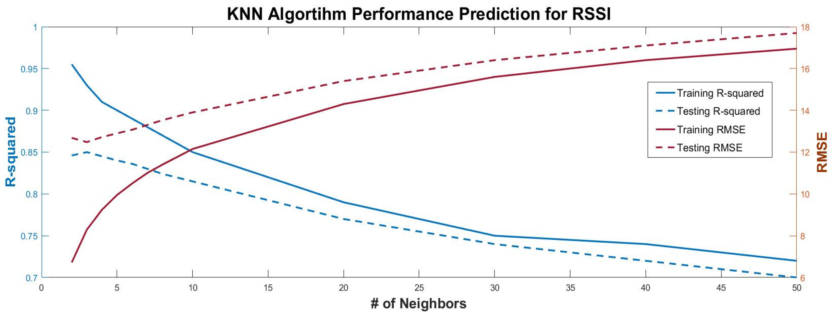
3.1. K-Nearest Neighbors Regression

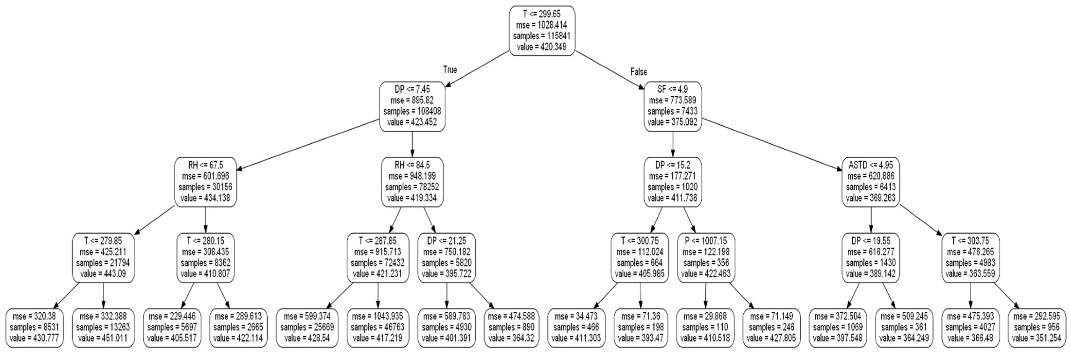
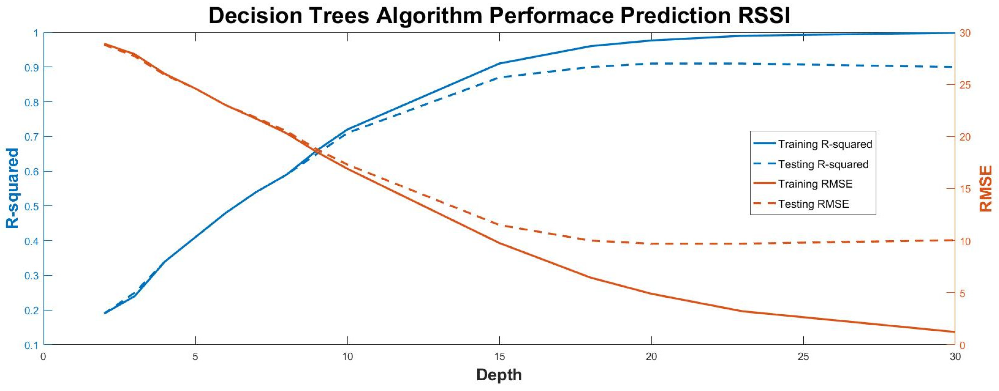
The KNN algorithm is a simple model to implement for regression and classification problems. To evaluate the effectiveness and adequacy of any algorithm, we need to account for (a) output interpretation ease, (b) calculation time and (c) power of prediction. The main advantages of KNN algorithm are the easiness of its output interpretation and the significantly low time for calculation. KNN is a simple algorithm that stores all available cases and predicts the numerical target based on a similarity measure (e.g., distance functions). A simple implementation of KNN regression is to calculate the average of the numerical target of the K nearest neighbors. Another approach uses an inverse distance weighted average of the K nearest neighbors. KNN regression uses the same distance functions as KNN classification. Choosing the optimal value for K is best done by first inspecting the data. In general, a large K value is more precise, as it reduces the overall noise; however, the compromise is that the distinct boundaries within the feature space are blurred. Cross-validation is another way to retrospectively determine a good K value by using an independent data set to validate the K value. Mathematically, the KNN regression algorithm can be expressed as the average of all training points in N₀, [29]:

$$f(x_0)=\frac{1}{\mathrm{K}}{\displaystyle \sum _{x_i\in N_0}{y}_i}$$

(5)

where x_i is the input and y_i is the output of the model, x₀ a prediction point and N₀ the K points that are closer to x₀. The coefficient of determination, R² and RMSE for our experimental data set are plotted against various numbers of neighbors (K) in Figure 4, starting from 2 up to 50. As shown in Figure 4, the coefficient of determination for the training subset initiates from a value of 0.95 and then gradually decreases to 0.75 when K = 50. The equivalent values for the testing subset had a peak value of 0.85 for K = 3, meaning that this is the optimal value for the number of neighbors that best fits KNN model to the data set; therefore, is the value we selected for our model A structured process of scanning the training subset (i.e., grid search) to determine the optimal value for a parameter is employed to determine the optimal K value (K = 3).

3.2. Decision Trees

A second simple and easy to interpret algorithm is the DT. Despite not so accurate comparing to other decision tree methods (e.g., random forests), gradient boosting is still a good alternative for regression and classification problems. This algorithm splits the predictor space into several regions and makes predictions based on the mean of the training observations of the corresponding region [29]. Starting from the root node, a decision tree is constructed via recursive partitioning. Each node is then split into two child nodes, based on the observation parameter that results in the maximum information gain. This process, known as recursive binary splitting, continues until the leaves are pure (i.e., samples at each node belong to the same class). The two basic steps of the DT process include the following [29]:

• Predictor space division into J distinct and non-overlapping regions, R₁, R₂, … R_J. The criterion to determine the optimal split point is to minimize the RSS given by,

  $${\displaystyle \sum _{j=1}^J{\displaystyle \sum _{i\in R_j}^{}{(y_i-y_{R_j})}^2}}$$

  (6)

  where y_Rj is the mean response for the training observations in the j-th box.
• For every observation falling into a certain region, the prediction emerges from the response mean value based on the training observations that belong to the same region.

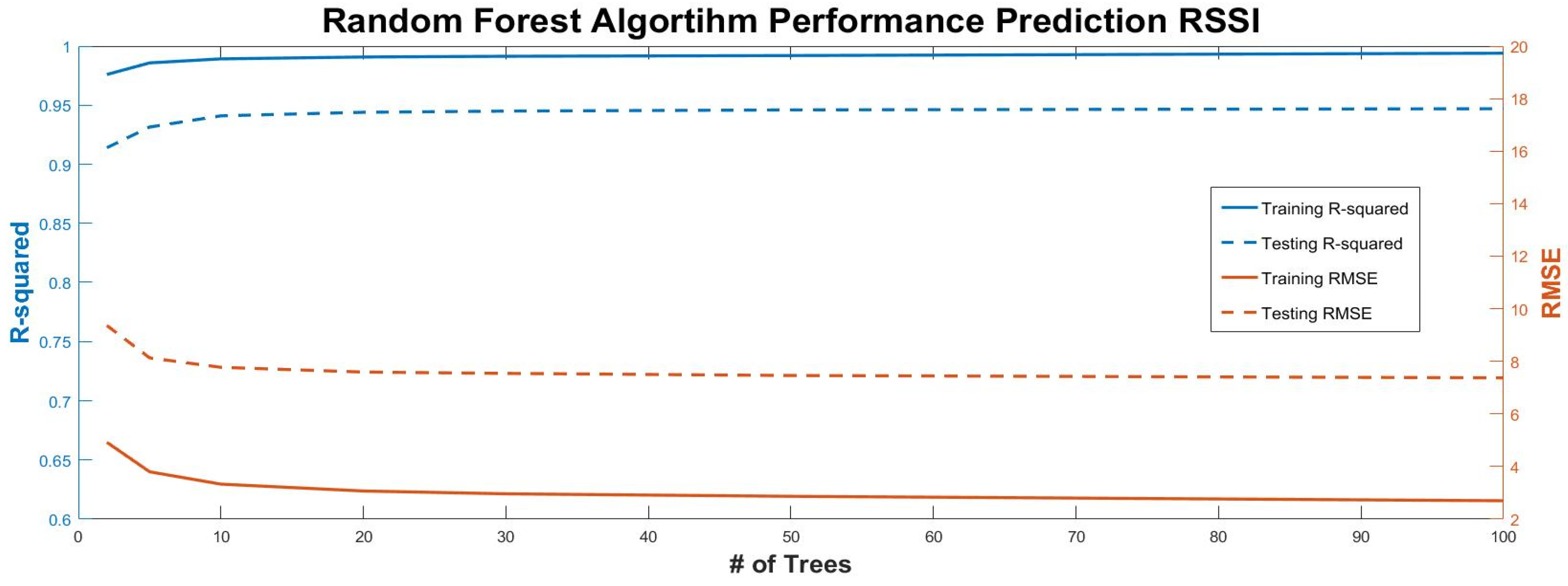
Figure 5 shows the first three levels of the decision tree to predict RSSI. The root node assigns observations where T ≤ 299.65 to the left branch with a corresponding mean RSSI value of 423.452. The right branch (i.e., false outcome) leads to a child node that is further split based on the solar flux value and a corresponding mean RSSI value of 375.092, as shown in more detail in Figure 6. That is, for any training observation that includes a solar flux parameter value less than 4.9, the left branch will be selected and the corresponding values for the dew point parameter will then be examined.

The process described above can be followed until different depth levels are reached. However, there is a critical number of levels that improve the fit to the training data but decreases the fit to the test data; in other words, an overfitting effect comes into play. This issue is shown in Figure 7, where up to a tree depth of nine, the training and testing R² values coincide. For larger tree depths, the testing R² values tend to converge to a value of 0.9 and no more improvement can occur. For this model, a tree depth of 20 is selected, as it provides the optimum performance metrics values for the testing subset. Larger tree depth values can result in a decrease of model performance.

3.3. Random Forest

The decision tree algorithm exhibits high variance that can correspond to less prediction accuracy. That means that if we apply a certain model built from the DT algorithm to different data sets, we will probably observe significantly different results. Instead, the prediction accuracy of a model with low variance would be consistent in any data set. To improve this issue, the method of bagging is applied to improve the DT algorithm’s performance. This method makes use of the general principle that averaging different sets of data will result in lower variance. Therefore, if we train our DT model for different samples from a single training data set and average their predictions, we will achieve a model with higher prediction accuracy.

The RF algorithm elaborates on this principle and by decorrelating the trees to achieve an even higher performance. The way to do so is by selecting only a random subset of predictors in each node split (approximately equal in value to the square root of the total number of the predictors), thus permitting less important predictors to play a role in the model construction. That being said, running a RF model by using the whole set of predictors at each split, will result in a simple bagged decision tree.

The results of running a RF algorithm in our data set, improved compared to the single decision tree method. A coefficient of determination, R², for the model evaluation of 0.95 is achieved and is indicative that this occurs with not so many different trees, as shown in Figure 8. Approximately, 20 different trees are sufficient to construct a model with the highest possible accuracy. Therefore, considering the lower complexity of a RF model with less trees and since more trees do not provide better results, we selected a value of 20 for our model. It is also important to notice that training and testing R² do not coincide for any number of trees; instead, there is a constant difference of 0.05. On the other hand, the RMSE begins with a value of 4.5 for two trees and rapidly reduces to less than 3 for the rest of the number of trees. A significant advantage of the RF algorithm is that by adding more trees we do not risk overfitting [29].

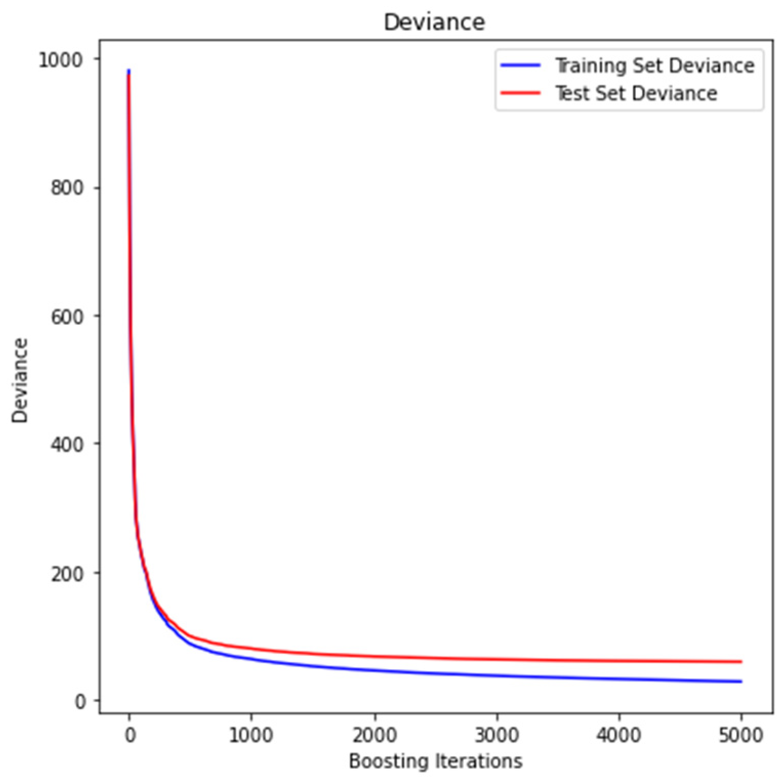
3.4. Gradient Boosting Regression

Another approach to improve prediction performance is gradient boosting, which can be applied to many machine learning methods [29]. The major difference of this approach is that instead of training the model concurrently, as is done in decision tree and random forest methods, it trains it sequentially. Specifically, the first decision tree is fitted to the training data set, the second is fitted using the residuals of the previous one, and then this new tree is added to the fitted function in order to update the residuals. This procedure is followed by fitting rather small trees -few number of terminal nodes- to the residuals, and that way we improve the model in areas where it does not perform as well. An additional shrinkage parameter λ exists that allows more and different trees to be fitted in certain areas where higher residuals appear.

We selected to fit our gradient boosting regressor model to our data set by using a tree number -iterations- of 5000 and a learning rate of 0.05. The model performed sufficiently and was comparable to the RF by achieving the value R² = 0.941 and an RMSE = 7.71. In Figure 9, the model improvement is illustrated in terms of predictive accuracy as compared to the boosting iterations, which in the case of regression problems equals the number of trees, since each iteration uses a single tree.

Impurity-based feature importance can be misleading for features with many unique values. As an alternative, we can compute the permutation importance. Permutation feature importance is a model inspection technique that can be used for any fitted estimator when the data is tabular, something very useful for non-linear estimators. The permutation feature importance is defined as the decrease in a model score when we randomly shuffle the value of a single feature [41]. This procedure breaks the relationship between the feature and the target; thus, the drop in the model score is indicative of how much the model depends on the feature. This technique benefits from being model agnostic and can be calculated many times with different permutations of the feature. For the current test subset, both the impurity-based and permutation methods -as a box-plot figure- identify the air temperature as the most significant predictive feature, whereas the rest of the ranking differs, as shown in Figure 10.

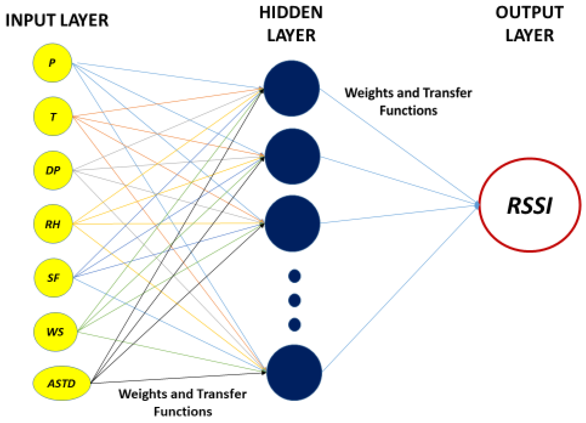
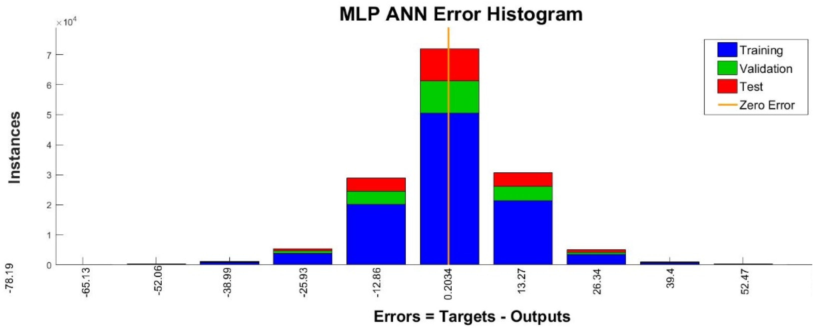
3.5. Artificial Neural Network

Another powerful form for ML model’s implementation is the ANN. An ANN resembles the function principles of a human’s brain. The analogy is that, in place of the brain neurons, an ANN model uses the nodes that deliver the signal’s information within the network. The basis of an ANN is the perceptron, which receives an input signal x_i with a weight of w_i and a bias b, added through a summation junction and then passed through an activation function f to provide the final output, as shown in Figure 11. All these complex combinations of input signals, weights, activation functions and biases for each layer allow for a sufficient modeling of highly non-linear relationships.

The perceptron transfer function can then be expressed as [42],

$$y=f({\displaystyle \sum _{i=1}^n{W}_{ji}{x}_i+b)}$$

(7)

The internal layer perceptrons, those in between the input and output layers, receive the summed weighed values of the input parameters (i.e., temperature, pressure, dew point, solar flux, wind speed, relative humidity and air-sea temperature difference) and provide the “input” signal for the output layer. All three layers are fully connected to each other. The proposed ANN architecture contains seven nodes in the input layer and a single node in the output layer RSSI, which receives the weighted input signals from the hidden layers along with a bias and represents the values of the predicted variable. The architecture of our model is a multi-layer perceptron model (i.e., shallow neural network) and the input-output mapping can be represented as follows:

$$y=g({\displaystyle \sum _{j=1}^{m_1}{W}_j}f({\displaystyle \sum _{i=1}^n{W}_{ji}{x}_i+b)}+c)$$

(8)

where g is the transfer function and c is the bias for the output layer. Other ANN architectures could include more than a single hidden layer. The transfer function to characterize the hidden layer, can be one of the following functions, [42]:

$$\mathrm{Tan}\mathrm{gent}\mathrm{Hyperbolic}\mathrm{Function}:f(x)=\frac{(e^x-e^{-x})}{(e^x+e^{-x})}$$

(9)

$$\mathrm{Sigmoid}\mathrm{Function}:f(x)=\frac{1}{1+e^{-x}}$$

(10)

$$\mathrm{Rectified}\mathrm{Linear}\mathrm{Unit}\left(\mathrm{ReLU}\right)\mathrm{Function}:f(x)=\max (0,x)$$

(11)

$$\mathrm{Gaussian}\mathrm{Function}:f(x)=e^{-x^2}$$

(12)

$$\mathrm{Linear}\mathrm{Function}:f(x)=x$$

(13)

We used a standard Levenberg-Marquardt learning method to train a two-layer feed-forward network with sigmoid hidden neurons and linear output neurons for an extended number of nodes (i.e., 2–100) in order to map the macroscopic meteorological parameters obtained from the weather station to the RSSI parameter obtained from the FSO system. The neural net fitting application of MATLAB was used to perform all the ANN computations.

The ANN algorithm applies a three-fold division of the entire data set (i.e., the training, validation and testing subsets). The training data subset is presented to the network during training and the network is adjusted according to its error. The validation subset is used to measure the generalization of the network and stop the training when generalization stops improving. The testing subset is used to independently measure the performance of the network after training. Seventy percent of the entire data set was assigned to the training of the network, fifteen percent to the training validation, and fifteen percent for the network’s performance testing. Figure 12 shows the performance of the MLP ANN algorithm for the RSSI prediction based on the seven meteorological parameters. We trained, validated and tested the algorithm for different numbers of nodes of the hidden layer, which resulted in significant decrease of the model prediction error approximately up to the 20th node. A further increase in hidden layer nodes provides slightly better results but also a substantially bigger computational cost. Figure 13 shows the error distribution for the training, validation and testing subsets, which appears to follow a normal distribution indicative of a very good performance of the prediction regression model, also shown in Figure 14, for a node number of 50 and a coefficient of determination R² = 0.921, both for the training and the testing phase.

3.6. Model Comparison and Discussion

Five ML algorithms were utilized to construct a predictive model for the RSSI parameter of an FSO link. The size of the data set and the considerable variance of the independent variables made the task of fitting a traditional linear or non-linear model (i.e., polynomial) very challenging. In particular, a second-order polynomial was initially fitted to the data set with a very poor performance, specifically an R² = 0.36 for the training subset and an R² = 0.05 for the testing subset. Therefore, more sophisticated models were required to achieve adequate prediction accuracy of the RSSI parameter. We trained and tested five different ML algorithms and used the determination of coefficient R² and RMSE as the performance metrics to evaluate each algorithm and compare among each other.

Table 2. Performance comparison of the baseline and five ML algorithm models for RSSI prediction in terms of R-squared (R²) and root mean square error (RMSE).

Approach		R2			RMSE
	Training	Validation	Test	Training	Validation	Test
Baseline	0.36	-	0.05	-	-	-
KNN	0.93	-	0.85	8.29	-	12.48
DT	0.9764	-	0.91	4.9	-	9.71
RF	0.994	-	0.947	2.7	-	7.37
GBR	-	-	0.9417	-	-	7.71
ANN	0.9496	0.9468	0.94867	10.06	10.19	10.17

summarizes the results for each model for the training, validation (if applicable) and testing phase. The ANN proved to be the most accurate model, with an R² = 0.94867 but also a very high computational time cost (it takes approximately 3 h to train, validate and test the model). On the other hand, all three tree-methods provided comparable results within a relatively short training period of time. Finally, the KNN algorithm resulted in a slightly less accurate model, yet it was much better than the polynomial model and was still statistically significant for RSSI prediction.

Comparing to previous studies, the ML algorithms that were used in this study proved to be much more robust and accurate than the polynomial model developed elsewhere [27,28], despite referring to a much larger data set that spanned over a year and included measurements from different seasons. As shown in Table 1, the value range of the measured meteorological parameters is much higher compared to those in [27,28]. However, the prediction accuracy performance of the models used in this study, outperformed the previous ones since they achieved an R² > 0.9, which is significantly higher comparing to an R²~0.7 of the previous models [27,28]. Regression models for RSSI prediction developed in [24,25] also did not achieve an accuracy higher than 70%. It is clear that the ML algorithms provide a more efficient method to predict the RSSI parameter of an FSO link. However, the ML algorithms provide in a less intuitive prediction model and require a deeper comprehension in order to interpret the results.

4. Conclusions

In this study, a machine learning based scheme was introduced to estimate the RSSI parameter of an FSO link over a maritime environment based on macroscopic meteorological measurements. To test the proposed approach, a large experimentally derived data set was used, which included seven parameters (i.e., air temperature, wind speed, solar flux, dew point, relative humidity, air pressure and air-sea temperature difference) obtained over a twelve-month period from a commercial FSO system and a weather station, respectively. Five popular ML algorithms were trained in order to construct a robust model to accurately predict the link’s performance in terms of received signal strength. The results showed a significant improvement compared to traditional regression modeling techniques (i.e. polynomials) and their prediction accuracy performance measured by the coefficient of correlation R² and the RMSE was extremely promising for even more complex predictive modeling. The significance of each of the independent variables was also studied with the gradient boosting regression algorithm by using two different approaches. Both of them showed that air temperature influences the output parameter the most. While all five ML methods showed a high degree of RSSI prediction accuracy, the ANN approach resulted in the most accurate model in terms of R² (i.e., 0.94867) while the RF in terms of RMSE values (i.e., 7.37). ANN and GBR did require a significant computational time, while the three other methods gave their results in a much shorter training time. Overall, this study provided a thorough insight to RSSI prediction accuracy using different machine learning methods that proved to be notably accurate to model such a relationship of complex mechanisms. The superlative performance of the ML approaches comparing to the common-used regression method indicates that, first, ML is the appropriate modelling choice when overall prediction is the goal and the volume of data is high; second, allows the ability to tune hyper parameters per ML approach to enable optimal performance; and, finally, the trained models can be either improved by adding more data or be used for continuous streamflow RSSI predictions.

References

1. Ghassemlooy, Z.; Popoola, W.O. Terrestrial Free-Space Optical Communications, Mobile and Wireless Communications Network Layer and Circuit Level Design; Fares, S.A., Adachi, F., Eds.; InTechOpen: London, UK, 2010; ISBN 978-953-307-042-1. [Google Scholar]
2. Khalingi, M.A.; Uysal, M. Survey on Free Space Optical Communication: A Communications Theory Perspective. IEEE Commun. Surv. Tutor. 2014, 16, 2231–2258. [Google Scholar]
3. Andrews, L.C.; Phillips, R.L.; Hopen, C.Y. Laser Beam Scintillation with Applications, 2nd ed.; SPIE Optical Engineering Press: Bellingham, WA, USA, 2001. [Google Scholar]
4. Majumdar, A.K. Free-space laser communication performance in the atmospheric channel. J. Opt. Fiber Commun. Rep. 2005, 2, 345–396. [Google Scholar] [CrossRef]
5. Kaushal, H.; Jain, V.K.; Kar, S. Free Space Optical Communication; Springer: New Delhi, India, 2017. [Google Scholar] [CrossRef]
6. Barrios, R.; Dios, F. Wireless Optical Communications through the Turbulent Atmosphere: A Review, Optical Communications Systems; Das, N., Ed.; InTech: Rijeka, Croatia, 2012; ISBN 978-953-51-0170-3. [Google Scholar]
7. Oh, E.S.; Ricklin, J.C.; Gilbreath, G.C.; Vallestero, N.J.; Eaton, F.D. Optical Turbulence Model for Laser Propagation and Imaging Applications. Proc. SPIE 5160, Free-Space Laser Communications and Active Laser Illumination III; SPIE: Bellingham, WA, USA, 2004. [Google Scholar] [CrossRef]
8. Oh, E.S.; Ricklin, J.C.; Gilbreath, G.C.; Doss-Hammel, S.; Eaton, F.D.; Moore, C.; Murphy, J.; Oh, Y.H.; Stell, M. Estimating Optical Turbulence Using the PAMELA Model. Proc. SPIE 5550, Free-Space Laser Communications IV; SPIE: Bellingham, WA, USA, 2004. [Google Scholar] [CrossRef] [Green Version]
9. Vetelino, F.S.; Young, C.; Grant, K.; Wasiczko, L.; Burris, H.; Moore, C.; Mahon, R.; Suite, M.; Corbett, K.; Clare, B.; et al. Initial Measurements of Atmospheric Parameters in a Marine Environment. Proc. SPIE 6215, Atmospheric Propagation III; SPIE: Orlando, FL, USA, 2006. [Google Scholar] [CrossRef]
10. Wasiczko, L.M.; Moore, C.I.; Burris, H.R.; Suite, M.; Stell, M.; Murphy, J.; Gilbreath, G.C.; Rabinovich, W.; Scharpf, W. Characterization of the Marine Atmosphere for Free-Space Optical Communication. In Proceedings of the SPIE 6215, Atmospheric Propagation III, Orlando (Kissimmee), FL, USA, 17 May 2006. [Google Scholar]
11. Gilbreath, G.C.; Rabinovich, W.S.; Moore, C.I.; Burris, H.R.; Mahon, R.; Grant, K.J.; Goetz, P.G.; Murphy, J.L.; Suite, M.R.; Stell, M.F.; et al. Progress in Laser Propagation in a Maritime Environment at the Naval Research Laboratory. Proc. SPIE 5892. Free-Space Laser Communications V; SPIE: Bellingham, WA, USA, 2005. [Google Scholar] [CrossRef]
12. Burris, H.R.; Moore, C.I.; Swingen, L.A.; Vilcheck, M.J.; Tulchinsky, D.A.; Mahond, R.; Wasiczko, L.M.; Stell, M.F.; Suite, M.R.; Davis, M.A.; et al. Latest Results from the 32km Maritime Lasercom Link at the Naval Research Laboratory, Chesapeake Bay Lasercom Test Facility. Proc. SPIE 5793. Atmospheric Propagation II; SPIE: Bellingham, WA, USA, 2005. [Google Scholar] [CrossRef]
13. Moore, C.I.; Burris, H.R.; Rabinovich, W.S.; Wasiczko, L.; Suite, M.R.; Swingen, L.A.; Mahon, R.; Stell, M.F.; Gilbreath, G.C.; Scharpf, W.J. Overview of NRL’s Maritime Laser Communication Test Facility. Proc. SPIE 5892. Free-Space Laser Communications V; SPIE: Bellingham, WA, USA, 2005. [Google Scholar] [CrossRef]
14. De Jong, A.N.; Schwering, P.B.; Benoist, K.W.; Gunter, W.H.; Vrahimis, G.; October, F.J. Long-Term Measurements of Atmospheric Point Spread Functions over Littoral Waters, as Determined by Atmospheric Turbulence. Infrared Imaging Systems: Design, Analysis, Modeling and Testing. Proc. of SPIE; SPIE: Cardiff, UK, 2012; Volume 8355. [Google Scholar]
15. Ali, R.N.; Jassim, J.M.; Jasim, K.M.; Jawad, M.K. Experimental Study of Clear Atmospheric Turbulence Effects on Laser Beam Spreading on Free Space. Int. J. Appl. Eng. Res. 2017, 12, 24. [Google Scholar]
16. Qing, C.; Wu, X.; Li, X.; Zhu, W.; Qiao, C.; Rao, R.; Mei, H. Use of weather and forecasting model outputs to obtain near-surface refractive index structure constant over the ocean. Opt. Express 2016, 24, 12. [Google Scholar] [CrossRef]
17. Qing, C.; Wu, X.; Li, X.; Huang, H.; Tian, Q.; Zhu, W.; Rao, R. Estimating the surface layer refractive index structure constant over snow and sea ice using Monin-Obukhov similarity theory with a mesoscale atmospheric model. Opt. Express 2016, 24, 18. [Google Scholar] [CrossRef]
18. Van de Boer, A.; Moene, A.F.; Graf, A.; Simmer, C.; Holtslag, A.A.M. Estimation of the refractive index structure parameter from single-level daytime routine weather. Appl. Opt. 2014, 53, 26. [Google Scholar] [CrossRef]
19. Frehlich, R.; Sharman, R.; Vandenberghe, F.; Yu, W.; Liu, Y.; Knievel, J.; Jumper, G. Estimates of Cn2 from numerical weather prediction model output and comparison with thermosonde data. J. Appl. Meteorol. Climatol. 2010, 49, 1742–1755. [Google Scholar] [CrossRef]
20. Bourazani, D.; Stasinakis, A.N.; Nistazakis, H.E.; Varotsos, G.K.; Tsigopoulos, A.D.; Tombras, G.S. Experimental Accuracy Investigation for Irradiance Fluctuations of FSO Links Modeled by Gamma Distribution. In Proceedings of the 8th International Conference from Scientific Computing to Computational Engineering, Athens, Greece, 4–7 July 2018. [Google Scholar]
21. Garrido-Balsells, J.M.; Lopez-Martinez, F.J.; Castillo-Vazquez, M.; Jurado-Navas, A.; Puerta-Notario, A. Performance analysis of FSO communications under LOS blockage. Opt. Express 2017, 25, 25278–25294. [Google Scholar] [CrossRef] [Green Version]
22. Kong, L.; Xu, W.; Hanzo, L.; Zhang, H.; Zhao, C. Performance of a Free Space Optical Relay-Assisted Hybrid RF/FSO System in Generalized M-Distributed Channels. IEEE Photonics J. 2015, 7, 5. [Google Scholar] [CrossRef]
23. Alheadary, W.G.; Park, K.-H.; Alfaraj, N.; Guo, Y.; Stegenburgs, E.; Ng, T.K.; Ooi, B.S.; Alouini, M.-S. Free-space optical channel characterization and experimental validation in a coastal environment. Opt. Express 2018, 26, 6614–6628. [Google Scholar] [CrossRef] [Green Version]
24. Latal, J.; Vitasek, J.; Hajek, L.; Vanderka, A.; Koudelka, P.; Kepak, S.; Vasinek, V. Regression Models Utilization for RSSI Prediction of Professional FSO Link with Regards to Atmosphere Phenomena. In Proceedings of the 2016 International Conference on Broadband Communications for Next Generation Networks and Multimedia Applications (CoBCom), Graz, Austria, 14–16 September 2016. [Google Scholar]
25. Hajek, L.; Vitasek, J.; Vanderka, A.; Latal, J.; Perecar, F.; Vasinek, V. Statistical prediction of the atmospheric behavior for free space optical link. In Proceedings of the SPIE 9614, Laser Communication and Propagation through the Atmosphere and Oceans IV, San Diego, CA, USA, 4 September 2015. [Google Scholar]
26. Lionis, A.; Cohn, K.; Pogue, C. Experimental Design of a UCAV-based High Energy Laser Weapon. Nausivios Chora J. 2016, 6, 3–17. [Google Scholar]
27. Lionis, A.; Peppas, K.; Nistazakis, H.E.; Tsigopoulos, A.D.; Cohn, K. Experimental Performance Analysis of an Optical Communication Channel over Maritime Environment. Electronics 2020, 9, 1109. [Google Scholar] [CrossRef]
28. Lionis, A.; Peppas, K.; Nistazakis, H.E.; Tsigopoulos, A.D.; Cohn, K. Statistical Modeling of Received Signal Strength for an FSO Channel over Maritime Environment. Opt. Commun. 2020, 489, 126858. [Google Scholar] [CrossRef]
29. James, G.; Witten, D.; Hastie, T.; Tibshirani, R. An Introduction to Statistical Learning with Applications in R; Springer: Berlin/Heidelberg, Germany, 2013. [Google Scholar]
30. Wang, D.; Song, Y.; Li, J.; Qin, J.; Yang, T.; Zhang, M.; Chen, X.; Boucouvalas, A. Data-driven Optical Fiber Channel Modeling: A Deep Learning Approach. J. Lightwave Technol. 2020, 38, 4730–4743. [Google Scholar] [CrossRef]
31. Liu, J.; Wang, P.; Zhang, X.; He, Y.; Zhou, X.; Ye, H.; Li, Y.; Xu, S.; Chen, S.; Fan, D. Deep learning based atmospheric turbulence compensation for orbital angular momentum beam distortion and communication. Opt. Express 2019, 27, 16671–16688. [Google Scholar] [CrossRef]
32. Amirabadi, M.; Kahaei, M.; Nezamalhosseini, S.A.; Vakili, V.T. Deep Learning for channel estimation in FSO communication system. Opt. Commun. 2020, 459, 124989. [Google Scholar] [CrossRef] [Green Version]
33. Lohani, S.; Glasser, R. Turbulence correction with artificial neural networks. Opt. Lett. 2018, 43, 2611–2614. [Google Scholar] [CrossRef]
34. Lohani, S.; Knutson, E.M.; Glasser, R.T. Generative machine learning for robust free-space communication. Commun. Phys. 2020, 3, 177. [Google Scholar] [CrossRef]
35. Mishra, P.; Sonali; Dixit, A.; Jain, V.K. Machine Learning Techniques for Channel Estimation in Free Space Optical Communication Systems. In Proceedings of the 2019 IEEE International Conference on Advanced Networks and Telecommunications Systems (ANTS), Goa, India, 16–19 December 2019; pp. 1–6. [Google Scholar] [CrossRef]
36. Jellen, C.; Burkhardt, J.; Brownell, C.; Nelson, C. Machine learning informed predictor importance measures of environmental parameters in maritime optical turbulence. Appl. Opt. 2020, 59, 6379–6389. [Google Scholar] [CrossRef] [PubMed]
37. Wang, Y.; Basu, S. Using an artificial neural network approach to estimate surface-layer optical turbulence at Mauna Loa, Hawaii. Opt. Lett. 2016, 41, 2334–2337. [Google Scholar] [CrossRef] [PubMed]
38. Haluška, R.; Šuľaj, P.; Ovseník, Ľ.; Marchevský, S.; Papaj, J.; Doboš, Ľ. Prediction of Received Optical Power for Switching Hybrid FSO/RF System. Electronics 2020, 9, 1261. [Google Scholar] [CrossRef]
39. Tóth, J.; Ovseník, L.; Turán, J.; Michaeli, L.; Márton, M. Classification prediction analysisof RSSI parameter in hard switching process for FSO/RF systems. Measurement 2017. [Google Scholar] [CrossRef]
40. Xu, R.; Lv, P.; Xu, F.; Shi, Y. A survey of approaches for implementing optical neural networks. Opt. Laser Technol. 2021, 136, 106787. [Google Scholar] [CrossRef]
41. Breiman, L. Random Forests. Mach. Learn. 2001, 45, 5–32. [Google Scholar] [CrossRef] [Green Version]
42. Cifuentes, J.; Marulanda, G.; Bello, A.; Reneses, J. Air Temperature Forecasting Using Machine Learning Techniques: A Review. Energies 2020, 13, 4215. [Google Scholar] [CrossRef]
Figure 1. The MRV TS5000/155 model FSO system in HNA (left), the maritime FSO link propagation path (center) and the FSO terminal on the lighthouse of Psitalia Island (right).
Photonics 08 00212 g001
Figure 2. Flow chart diagram for the ML-based methodology for FSO system RSSI modeling.
Photonics 08 00212 g002
Figure 3. Matrix of linear correlation coefficients for measured meteorological parameters and RSSI.
Photonics 08 00212 g003
Figure 4. Performance metrics plot for KNN algorithm against different number of neighbors.
Photonics 08 00212 g004
Figure 5. Decision Tree model for RSSI prediction. Each node depicts the split selection parameter, the resulted mean squared error (MSE) of the split, the number of samples included to the specific region and the mean RSSI value based on the samples of the region.
Photonics 08 00212 g005
Figure 6. Resulting child node for RSSI.
Photonics 08 00212 g006
Figure 7. Performance metrics plot for decision tree algorithm against different number of neighbors.
Photonics 08 00212 g007
Figure 8. Performance metrics plot for random forest algorithm against different number of trees.
Photonics 08 00212 g008
Figure 9. Training and testing MSE as n trees are added to the GBM algorithm.
Photonics 08 00212 g009
Figure 10. Feature importance (left) and permutation importance (right) for the GBR model estimators.
Photonics 08 00212 g010
Figure 11. The multilayer perceptron network architecture for RSSI prediction.
Photonics 08 00212 g011
Figure 12. Performance metrics plot for MLP ANN algorithm against different number of hidden layer’s nodes.
Photonics 08 00212 g012
Figure 13. Error histogram of the proposed ANN architecture for RSSI prediction for the training, validation and testing phases.
Photonics 08 00212 g013
Figure 14. Regression Fits for the proposed ANN architecture for RSSI prediction.
Photonics 08 00212 g014