Maintaining Constant Pulse-Duration in Highly Dispersive Media Using Nonlinear Potentials


Laser Physics and Nonlinear Optics Group, Department Science & Technology, MESA+ Research Institute for Nanotechnology, University of Twente, 7500 AE Enschede, The Netherlands
Photonics 2021, 8(12), 570; https://doi.org/10.3390/photonics8120570
Submission received: 17 November 2021
/
Revised: 6 December 2021
/
Accepted: 9 December 2021
/
Published: 11 December 2021
Abstract
:A method is shown for preventing temporal broadening of ultrafast optical pulses in highly dispersive and fluctuating media for arbitrary signal-pulse profiles. Pulse pairs, consisting of a strong-field control-pulse and a weak-field signal-pulse, co-propagate, whereby the specific profile of the strong-field pulse precisely compensates for the dispersive phase in the weak pulse. A numerical example is presented in an optical system consisting of both resonant and gain dispersive effects. Here, we show signal-pulses that do not temporally broaden across a vast propagation distance, even in the presence of dispersion that fluctuates several orders of magnitude and in sign (for example, within a material resonance) across the pulse’s bandwidth. Another numerical example is presented in normal dispersion telecom fiber, where the length at which an ultrafast pulse does not have significant temporal broadening is extended by at least a factor of 10. Our approach can be used in the design of dispersion-less fiber links and navigating pulses in turbulent dispersive media. Furthermore, we illustrate the potential of using cross-phase modulation to compensate for dispersive effects on a signal-pulse and fill the gap in the current understanding of this nonlinear phenomenon.
1. Introduction
Soliton formation, whereby an optical pulse does not temporally disperse in a medium, is of central importance to ultrafast optical physics. For example, the invariant temporal profile of solitons ensures that neighboring pulses of a data transmission train do not smear into each other, preventing the loss of information, and thus increasing data transmission rates [1,2].
A soliton occurs when the nonlinear additive phase through the Kerr effect is balanced with the additive phase from waveguide dispersion across the temporal profile of the pulse. Thus, a soliton occurs with a specific amplitude profile, i.e., a hyperbolic secant, and pulse energy set by the waveguide dispersion and nonlinear coefficient [3]. Usually, the dispersion of the waveguide must have negligible higher than second-order terms, limiting the generation of solitons to highly specific waveguides.
The need for preventing dispersive broadening of pulses in the presence of highly fluctuating group-velocity dispersion, such as for spectral regions around waveguide resonances, or at the edge of the stop band of Bragg-gratings, is becoming more significant with emerging technologies [4,5,6]. Many new optical technologies in the integrated platform use a bus waveguide coupled to ring resonators; for example, for optical sensors, lab-on-a-chip, filters, optical delay lines, and even as an optical memory scheme [7,8,9,10,11]. However, these resonant absorptive features introduce highly fluctuating dispersion both in magnitude and sign across a moderate frequency range, through the corresponding Kramers–Kronig relations. Thus, signal pulses that are not meant to be coupled to these resonators, but are close to the resonances, suffer extreme dispersive effects, which may limit the versatility and frequency range of these integrated platforms.
The non-dispersing ultrafast pulse being limited to high-pulse energies is also a problem that must be resolved in the context of new technologies. For example, for quantum technologies, a low pulse energy far below the nonlinear threshold is present [12,13]. Therefore, the only way to limit dispersive smearing of the signal pulses is by linear methods such as pre-chirping the spectral phase.
In these linear methods, the conjugate spectral phase is imposed on the input pulses to the total generated spectral phase by dispersion seen at the end of the waveguide. However, these linear methods are lossy—which substantially increases the integration times or even destroys information for single-photon quantum technologies [14,15,16,17]. Moreover, they can only compensate for one location on the waveguide (e.g., fiber) network and information cannot be routed to many different locations without being distorted.
Given the above discussion, it would be highly beneficial to obtain a method to generate close to ‘stationary’ pulses for arbitrary profiles, in any dispersion landscape at low pulse energy, where the duration remains approximately the same for the entire propagation. In this paper, we formulate and show, through numerical examples, a method to prevent temporal broadening of pulses of more arbitrary shapes and energies in a manner less dependent on the waveguide’s dispersion profile than current soliton generation allows.
We do this by controlling a weak-amplitude signal-pulse (for example, the single-photon in quantum technologies) with a much stronger ‘control’ pulse that offers an optical potential that induces cross-phase modulation (XPM). The control pulse may be at the same carrier frequency as the signal pulse, but at an orthogonal polarization, or at a carrier frequency at a large offset to the signal pulse, such that the dispersion landscape of the control pulse is not as turbulent as the signal pulse. While XPM of two pulses has been explored before, it has only been explored for limited pulse profiles (such as for two soliton pulses) or in the context of frequency shifting a signal pulse with the control [18,19,20,21,22,23]. Our method adds a versatile XPM technique for various dispersion landscapes and pulse profiles.
To showcase our method, we present two examples. The first shows how an ultrafast signal pulse can avoid dispersive effects in highly fluctuating (across five orders of magnitude) group-velocity dispersion, such as within the resonance regions of a waveguide. In this example, the control pulse is separated by a large frequency offset, such that it is in a non-fluctuating dispersion ‘zone’ (e.g., far from a resonant feature or far into the passband of a Bragg grating). The second example shows how a low-energy ultrafast signal-pulse, e.g., a single photon, can avoid dispersive broadening in a practical widely used telecom fiber. Here, the control pulse is at an orthogonal linear polarization state, but at the same central frequency with the signal pulse. Thus, the control pulse can be separated from the single photon by polarization filtering.
We highlight the general case where our method can be of great use by setting that, in both examples, the control pulse, having the allowance of being at high-energy, can be generated by techniques that are lossy. However, the signal pulse is constrained to low-energy and cannot be shaped by the same techniques.
The method is then generally ideally suited for controlling the temporal wave-function of ultrafast weak signals like single-photons in a loss-less approach through a wide variety of highly dispersive or standard waveguides. Other applications include overcoming—or switching dispersive effects in an ultrafast manner—for example, in resonant waveguides or Bragg stacks. The method can be used to significantly increase the transmission rate of telecommunications, where the limitation arises as a result of dispersive smearing of the pulse train.
The analytical expression for the exact control-pulse profile needed given an arbitrary or general signal-pulse profile is shown. The control-pulse shape that would generate the conjugate temporal phase to the one from dispersion is obtained, such that the two cancels to near zero for the signal-pulse at any point in the propagation.
Ultimately, this allows for near invariant temporal solutions across a wide range of signal-pulse shapes and dispersion profiles. The method then fills the gap in our understanding of XPM-induced control of temporal broadening.
2. Methods and Theory
We start by deriving the method’s expressions used to obtain the control-pulse needed for maintaining a stationary signal-pulse. We restrict our analysis to the waveguide case, where only the propagation spatial dimension needs to be considered. The nonlinear equations of motion of two pulses, separated in central frequency or polarization, with complex envelope functions (control-pulse) and (signal-pulse) undergoing XPM, are given in Equations (1) and (2) [24]:
We impose that is much larger than and that the signal-pulse has a small amplitude, such that it does not contribute to any nonlinear effects. Therefore, Equations (1) and (2) reduce to the indicated approximate forms. and are the dispersive coefficients, arising from the frequency-dependent wavenumber Taylor expanded about the control or signal’s central frequency or . is the pulse time-coordinate defined in a co-moving frame-of-reference.
The above system equations are solved to obtain the control-pulse envelope profile giving a stationary solution of the signal-pulse. However, a few conditions must be met, which we list before indicating the derivation:
(1) The dispersive broadening of the control-pulse must be negligible, i.e., in the dispersion length, [6], is the input pulse duration and must be larger than the interaction length of the two pulses.
(2) The group-velocities of both pulses, and , are the same. This means that the group-delay at the control-pulse’s central frequency, i.e.,
In the above, is the wavenumber and is the frequency dependent group-velocity dispersion seen by the control- and signal-pulse. is the frequency corresponding to the group-velocity of the common moving time frame-of-reference of the two pulses. For the remainder of this paper, we take a frame-of-reference co-moving and centered with the control-pulse.
Many dispersion profile arrangements could satisfy Equation (3). Thus, matching the group-velocity of the pump and signal is not constrained to a highly specific waveguide geometry or material. The non-constrained nature of GV-matching is illustrated by the large amount of existent literature wherein nonlinear effects such as second harmonic generation and cross-phase modulation are observed [25,26,27,28,29]. In fact, for radially symmetric waveguides (such as fiber), a simple trick to ensure the same group-velocity is to set the pump and signal pulse to orthogonal polarizations, as done in Section 3.2.
Likewise, the condition that dispersive effects of the control pulse are negligible—in comparison with those seen by the signal pulse—is satisfied by a wide variety of waveguides explored in past studies. For example, at the zero-dispersion point (or region) of photonic crystal fibers or at a wavelength range in the detuned region of a Bragg grating structure [30,31,32,33]. This would then be the location of the control pulse. However, for other wavelengths, the dispersion profile can oscillate by orders of magnitude specially around resonances of the waveguide system (for example, see [34] or within the bandgap of a Bragg-grating structure). Thus, the oscillating part of the dispersion profile would be where the signal pulse is located (as a corollary, the signal pulse and control pulse would usually then have central wavelengths separated by a large range). Such general systems, where the dispersion is turbulent for a signal pulse, but well-behaved for a control-pulse, are the discussion point of Section 3.1.
2.1. Control-Pulse Formulation
The first step in formulating the required control-pulse is to insert the following Ansatz ( is a constant) into Equation (2). The approximation is also inserted—which is exact if there is no dispersive broadening for the control-pulse. Rearranging to solve for and dividing out the common yields
As the left-hand side of Equation (4) equates to a positive definite function for all , so must the right-hand side. From this positive definitive condition, is a real constant and it can be shown that the signal-pulse must always be in a form , where is a transform limited complex amplitude function and is a constant. Generally, , to guarantee that the left-hand side can never be negative. The value of can be arbitrarily chosen, as long as it satisfies this inequality. However, minimizing would minimize the maximum of , thus minimizing the control pulse’s energy. For the remainder of the paper, we then take .
It seems, mathematically, that another condition needed for Equation (4) to be valid is that the odd-dispersion coefficients must be zero, at least for the dispersion profile that covers the signal-pulse’s bandwidth. Thus, across the bandwidth of the signal-pulse, the dispersion profile is ideally symmetric about the central wavelength—e.g., for ultrashort <100 fs pulses, the dispersion profile should be symmetric across a bandwidth range less than 50 nm. There are a plethora of waveguides that satisfy this symmetry requirement from dispersion engineered photonic crystal fibers to the system described in [35]. Furthermore, we find from full numerical simulations that the symmetry condition is not strictly necessary (see Section 3 for related discussion) and introduces little error for moderate odd-order dispersion coefficients (taken about the central wavelength of the signal) if Equation (4) is modified to Equation (5), given as follows:
even if this modification is not supported in a strict mathematical sense.
Equation (4) indicates that can be a product between any real function and exponential phase function, as only the absolute magnitude must obey the equation. Values of that lie outside of the temporal profile of the signal-pulse, , can equal zero or any convenient function without additional error.
2.2. Deviation from Stationary Propagation
In a practical setting, as Equation (4) consists of a quotient term, it may be necessary to truncate it for large when goes to zero. The truncation is decided by the desired energy upper bound that the control-pulse must satisfy. Thus, is uncontrolled for larger than the truncation window, yielding the potential error of dispersive broadening in the wings of the signal-pulse.
For example, it can be shown that, for a Gaussian pulse, , Equation (4) becomes
where are the set of Physicists Hermite Polynomials [36] of order .
When only second-order group-velocity dispersion is present, Equation (6) equates to a parabolic function, and thus does not converge uniformly to zero. Thus, the edges of a Gaussian pulse may temporally disperse away from the XPM controlled central region of the signal-pulse. This limitation will be explored in the subsequent section.
3. Results
3.1. Example 1: Near Stationary Pulses in Turbulent Dispersive Media
To understand both the limitations and impact of the above theoretical procedure for XPM-induced stationary pulse propagation, we consider pulse propagation in a turbulent dispersive waveguide medium. We restrict our analysis to the waveguide case, as diffraction is negligible and can be omitted from the analysis. The diffractive term of the full three-dimensional NLSE, for example, shown in [37], cannot be accounted for by the method used to obtain Equation (4).
To solve for the dynamics of the pulses undergoing nonlinear propagation in the turbulent waveguide, we first use Equation (5) to generate the amplitude function of the control-pulse given a certain signal-pulse we want to propagate invariantly. We then numerically solve, using the split-step Fourier method [24], the coupled NLSE equations (Equations (1) and (2)) for both pulses, with the input control and signal profile as initial conditions.
The turbulent dispersive waveguide medium we study is defined as having narrow fluctuations between positive and negative GVD spanning orders of magnitude within a small bandwidth of frequencies. We apply our method for turbulent dispersion because the highly fluctuating dispersion demonstrates the full effectiveness and potential of our method, i.e., the large dispersion fluctuations would make controlling the associated dispersive effects challenging. While we show our method in this extreme case, we find our method is effective for more moderate examples too, such as pulse propagation through a telecom fiber with modest higher-order dispersion.
Impactful examples of such highly fluctuating dispersion that occur in many optical applications are generally when the frequency range of a pulse covers a waveguide’s absorption dip and/or gain peak or covers waveguide resonances, e.g., from leaky modes or evanescent coupling to neighboring waveguides. Such a case can occur for an ultrafast pulse (i.e., covering a large bandwidth) traveling through a doped waveguide that amplifies light while also coupled to a ring resonator detuned from the gain profile [38]. Another significant case is when a pulse travels in a waveguide where the Stokes peak location and absorption dip location (Stokes-shift) from the Raman effect are situated within the bandwidth of the original pulse [39].
To illustrate the control of temporal broadening within turbulent dispersive media, we have constructed an artificial waveguide that possesses a weak absorption and gain resonance characteristic of leaky mode strand resonances in photonic crystals [34]. The features are characterized by a Lorentzian gain peak and absorption dip within the bandwidth of an ultrafast (200 fs) pulse, where the pulse has a carrier frequency that sits precisely at the midpoint of these features. We take as the Lorentzian parameters used, the typical values from leaky mode strand resonances in photonic crystal fibers given in [34]. While we show an example with only two resonant features, we have also studied waveguides consisting of a series of multiple resonances, whereby the pulse bandwidth is centered such that the dispersion profile is symmetric within its bandwidth.
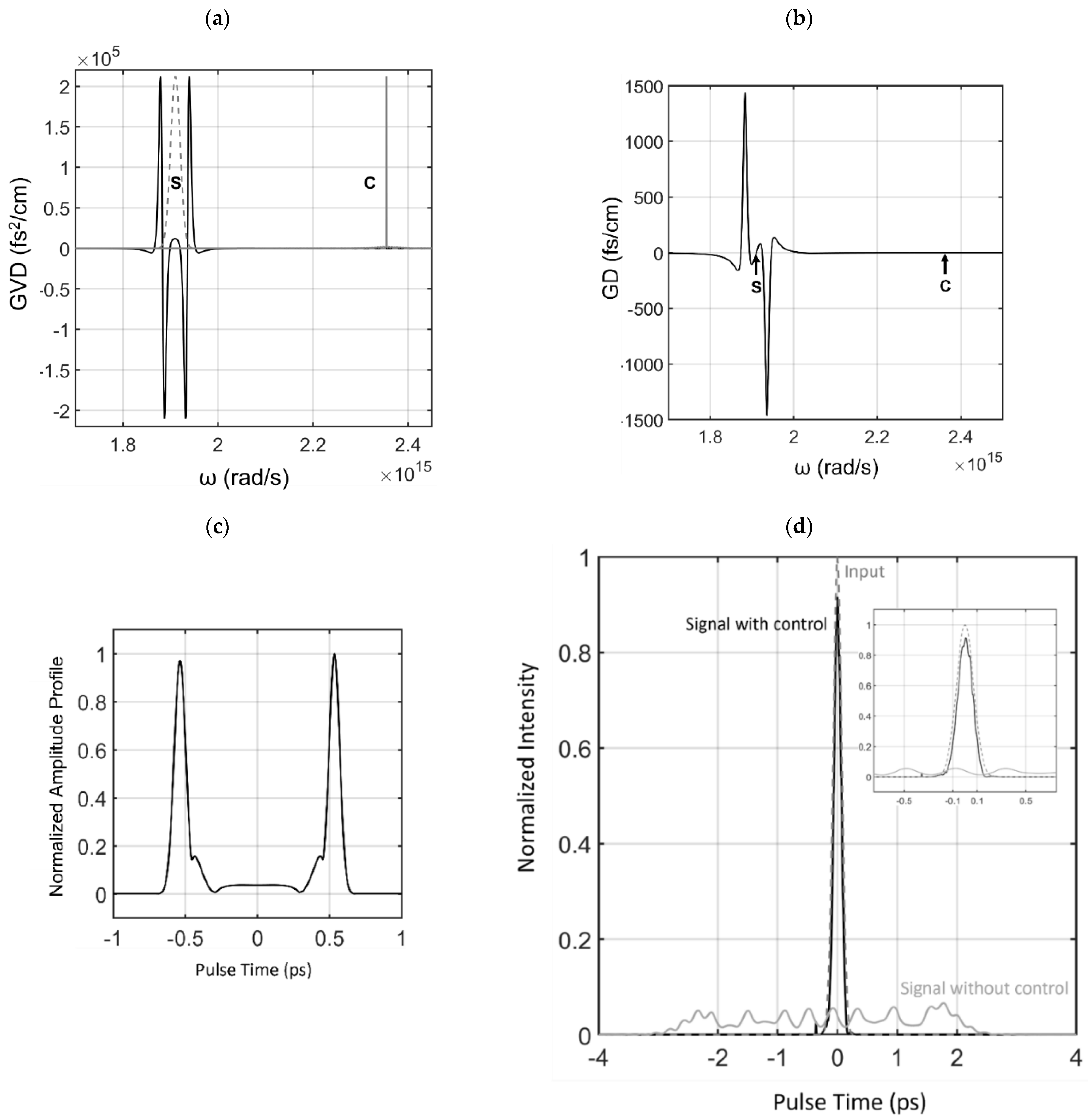
The waveguide has a flat-zero GVD when the absorption and gain are neglected. Through the associated Kramers–Kronig relations, the group-velocity dispersion is derived in the waveguide and is shown in Figure 1a along with the signal and control’s normalized spectral energy density distributions. The dispersion is symmetric around the signal-pulse’s carrier frequency and fluctuates over five orders of magnitude. To isolate and study the influence of dispersion on the control pulse energy, we take the same nonlinear coefficient () as is used with the next example in telecom fiber that has considerably less dispersion than the waveguide in this section.
The interaction of the highly fluctuating dispersion with our set of signal-pulses provides a stringent test for how well the XPM modulated signal-pulse avoids temporal broadening. To evaluate the quality of the controlled signal-pulse, we compare it to the signal’s temporal profile when there is no control-pulse. This comparison is done for three different signal-pulse types to show that our method works for arbitrary signal-pulses.
To isolate the dynamics of the signal-pulse, we center the control-pulse in a zero-dispersion region such that dispersive distortion of the amplitude profile is not present. Furthermore, both signal and pulse propagate at approximately the same group-velocity with negligible walk-off, as shown in the group-delay versus frequency, i.e., Figure 1b.
We now proceed with our first signal-pulse example, which is a 200 fs Gaussian pulse. The corresponding amplitude profile of the control-pulse is shown in Figure 1c, with an energy of approximately 11 µJ. In general, we find that the control-pulse energy scales directly with the order of magnitude of the dispersion fluctuations, going to nJ’s for lower dispersion magnitudes, e.g., on the order of 100 s of (as seen in the next telecom fiber example).
After 25 cm of propagation in the medium, the XPM controlled signal-pulse remains close to the Gaussian input pulse in profile and duration, as shown in Figure 1d. For comparison, the signal without the control-pulse is also shown, where it temporally broadens to a window of 6 ps and is highly distorted from the original Gaussian profile.
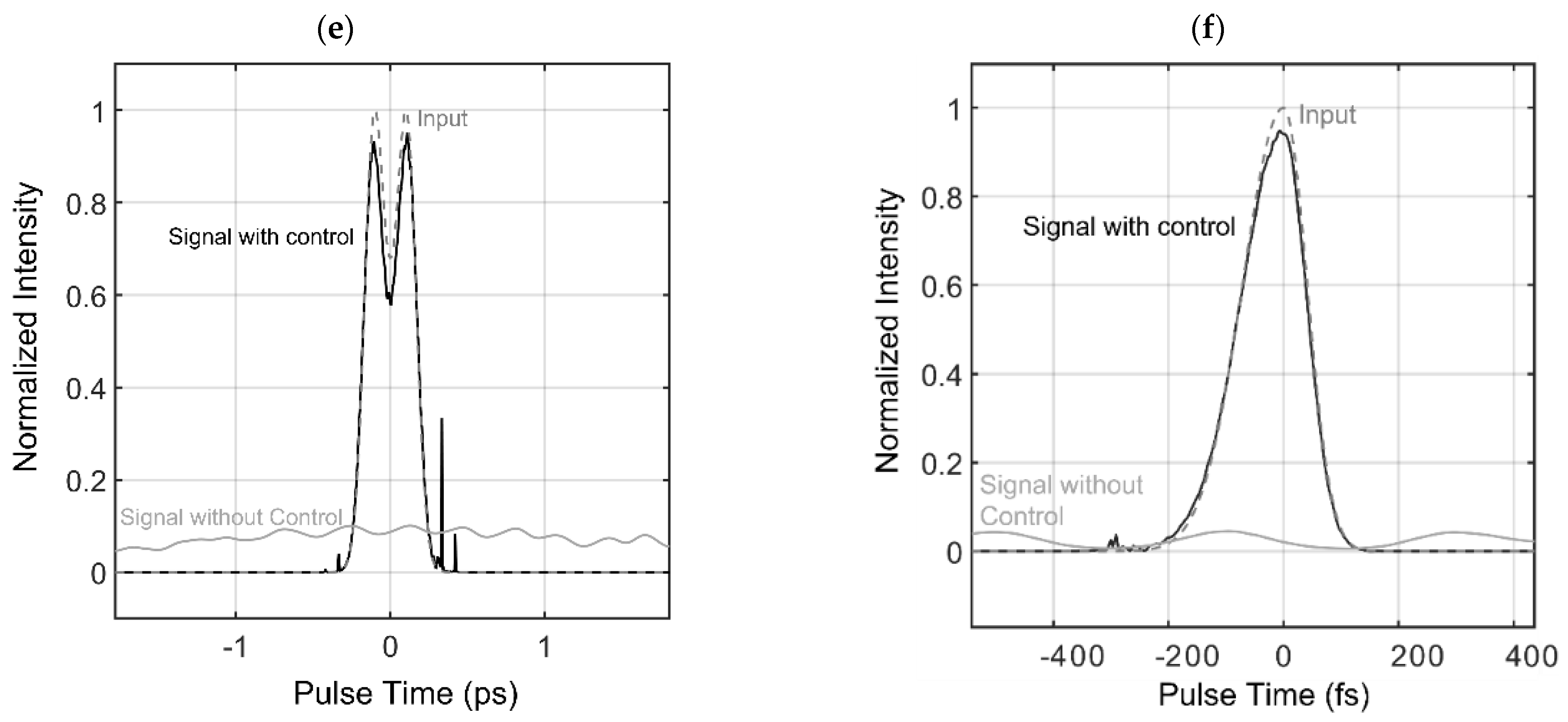
The next signal-pulse example is far from the typical Gaussian shape, as shown in Figure 1e. However, as in the Gaussian pulse case, the pulse maintained its duration and shape close to the input profile’s parameters when its corresponding control pulse (shown in Appendix B, Figure A2a, and with its -value given in Table A1) was applied. Without the corresponding control-pulse, the pulse would be highly distorted in shape, stretching out to 5 ps.
We then proceed with the last example, which is an asymmetric pulse that is slanted towards positive pulse time, as shown in Figure 1f. The corresponding control pulse profile is shown in Appendix B, Figure A2b, and its -value is listed in Table A1. As with the previous cases, the XPM controlled signal-pulse is close to the input profile at the end of propagation, while the uncontrolled case distorts considerably and stretches to approximately 6 ps.
Interestingly, the effects of the uncontrolled wings of the pulses (see Section 2.1 for associated discussion) can be seen as a slightly reduced pulse duration from the input pulse and small amplitude pre/post pulses (below the −4 dB level). This type of error then contributes primarily to the outcome of pulse compression instead of broadening, which is desirable for many applications. The dynamics at the temporal edge regions of the control-pulse explains the emergence of these deviations.
The edge locations of the control-pulse are defined when the input signal-pulse goes below an absolute amplitude value of −50 dB. The so-defined decaying edges of the control-pulse introduce a chirp profile that compresses the dispersively chirped temporally broadening wings of the signal-pulse and can even break them into sub-pulses as they interact with it, causing the overall pulse compression.
Moreover, there is a slight mismatched group-velocity of the signal with control-pulse attributable to numerical error. The error results from numerically integrating the GVD over a coarse grid, to obtain the group-velocity as a function of frequency. Though small, the mismatch produces XPM-induced wavebreaking [40] that adds small modulations on one side of the pulse profiles. This numerical error also enhances the error from the edge effects. Resorting to a finer grid for the GVD would resolve this numerical effect, at the expense of needing larger computational sources.
We provide a video of the second example pulse’s propagation across the waveguide in the Supplementary Information (Video S1). The video illustrates the maintained duration and shape of the signal-pulse with control.
3.2. Example 2: Preventing Dispersive Effects in Practical Telecom Fiber
The previous section shows how the method can control pulses in highly dispersive media. However, a noteworthy trait of the illustrated waveguide GVD in Section 2 is that it is symmetric about the signal pulse’s bandwidth, as this is a requirement for Equation (4). This section will explore a modification of Equation (4), given as Equation (5), in order to account for cases where there is an asymmetric dispersion profile for the signal pulse.
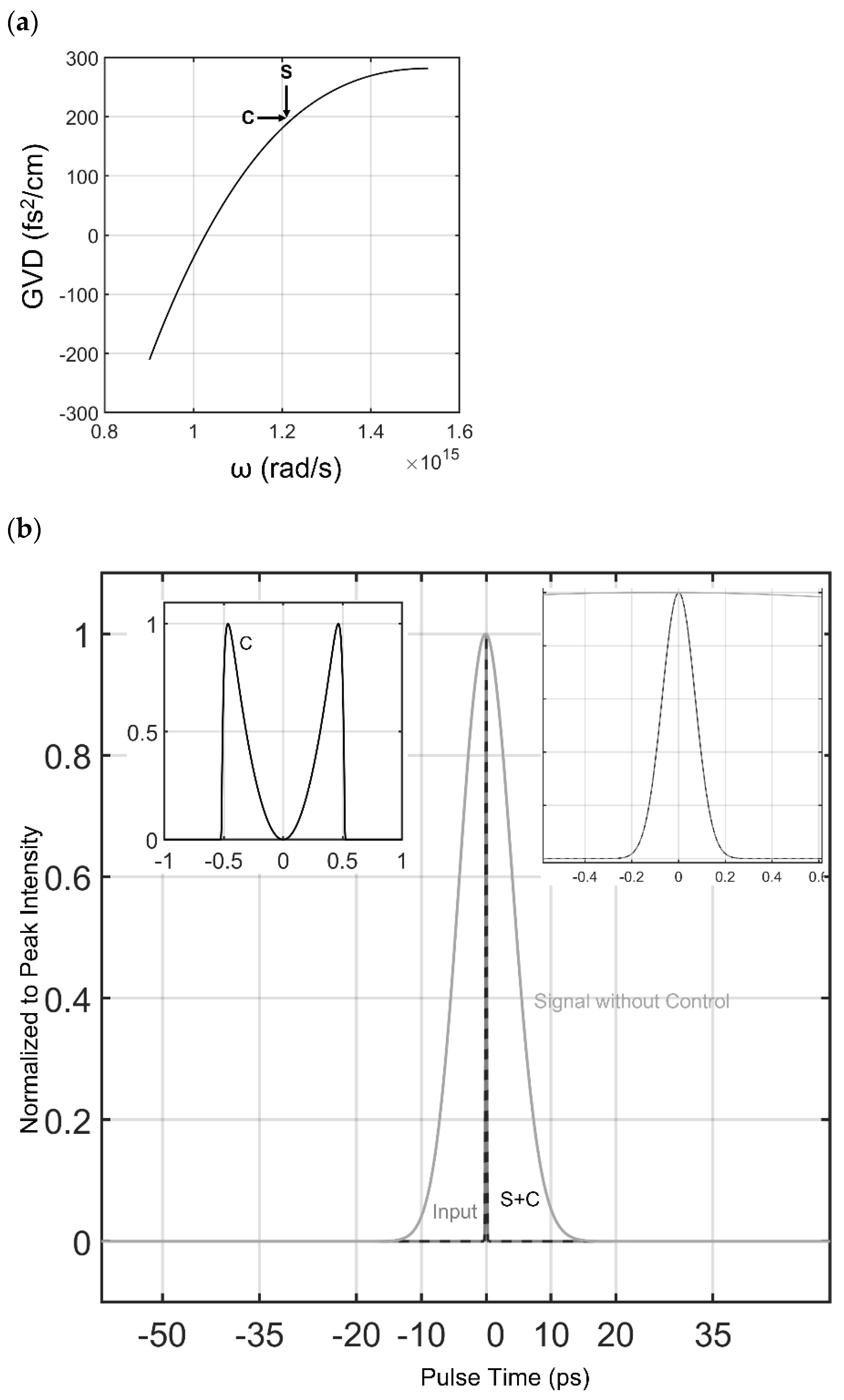
To illustrate how our method can work when there is moderate odd-order dispersion, we take the GVD profile and the nonlinear coefficient of a well-known radially symmetric step-index fiber found in many telecom applications [41]. The dispersion profile of the fiber so-named “Corning Hi1060Flex” is given in Figure 2a. As can be seen in Figure 2a, the fiber has normal dispersion for the frequency range considered and there is a large asymmetry in the GVD profile of the fiber, about the location of the signal pulse central wavelength. In this study, we set the control and signal pulse to the same wavelength, but orthogonal polarizations, so that they can still interact through cross-phase modulation. As both signal and pulse see the same dispersion profile, the group-velocities are matched.
3.2.1. Asymmetric Dispersion across Signal Pulse
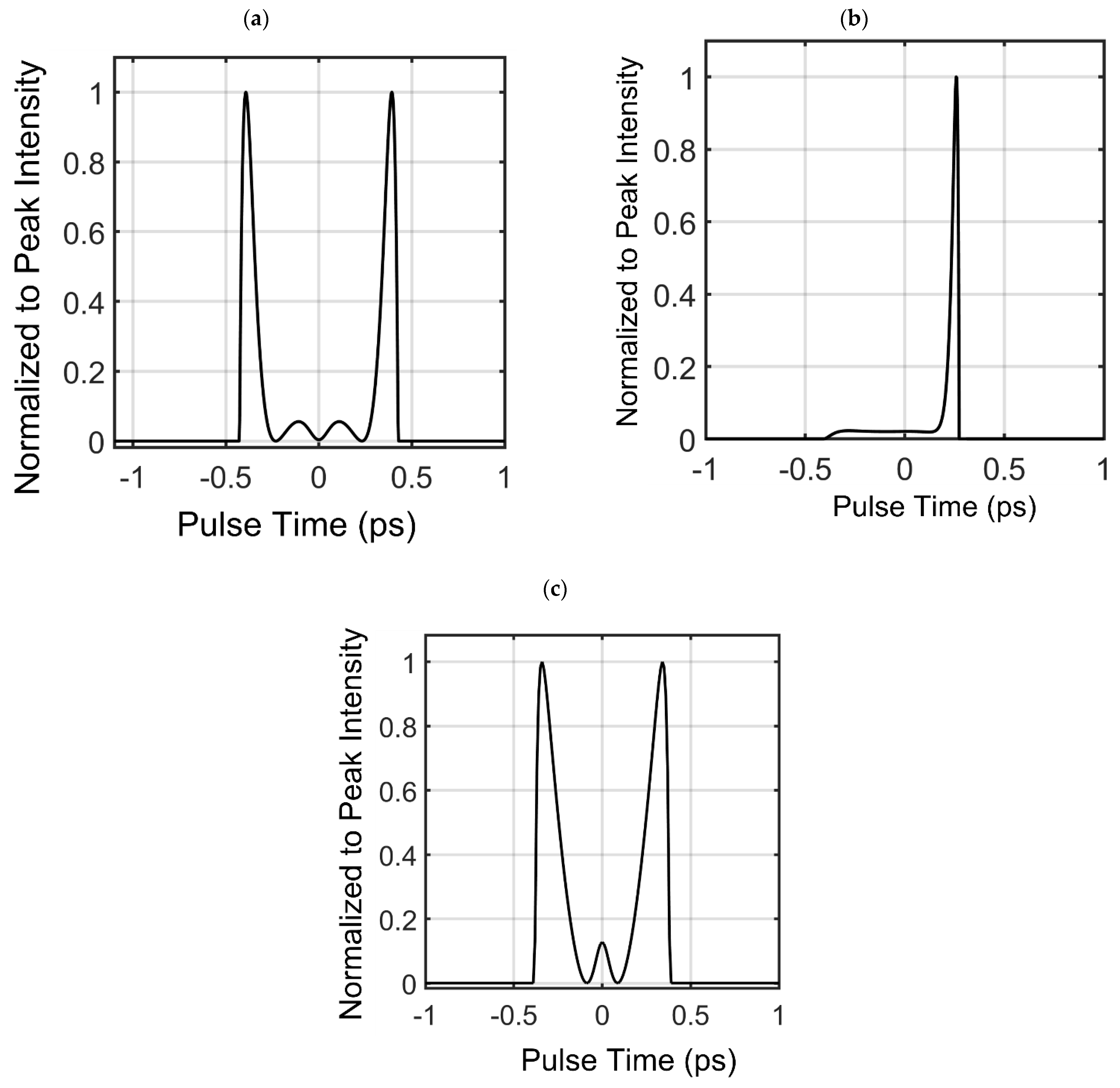
We start by propagating a signal and control pulse, dictated by Equation (5), across 30 m of the fiber waveguide. The signal pulse bandwidth is in a dispersion region where the dispersion profile is asymmetric about the pulse’s central wavelength, and thus possesses moderate odd-order dispersion coefficients when Taylor expanded around this central wavelength. For this section, the control pulse’s dispersive effects are turned off to properly illustrate the dynamics of a signal pulse centered in a non-symmetric dispersion profile range.
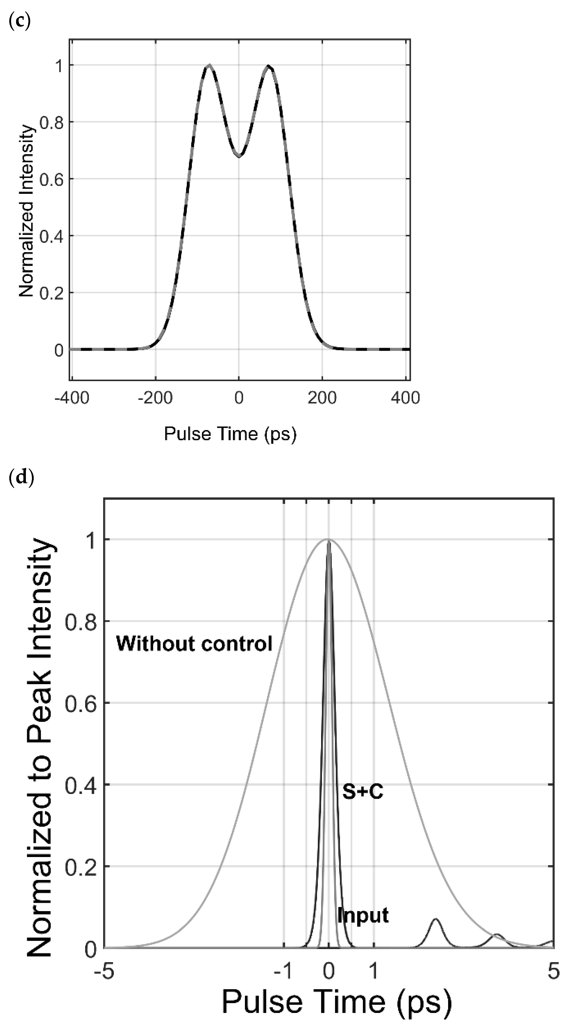
Figure 2b,c show that the control pulse successfully prevented the signal pulse from dispersing, for a variety of signal pulse shapes (Gaussian, two-peak pulse), to show the general validity of the method. For comparison, the signal without control is shown in Figure 2b, indicating large dispersive effects with no control pulse present. The specific control pulse for the signal pulse shown in Figure 2c and the associated p-values are given in Appendix B in Table A1 and Figure A2c.
3.2.2. Asymmetric Dispersion across Signal Pulse and Significant Presence of Dispersive Effects for Control Pulse
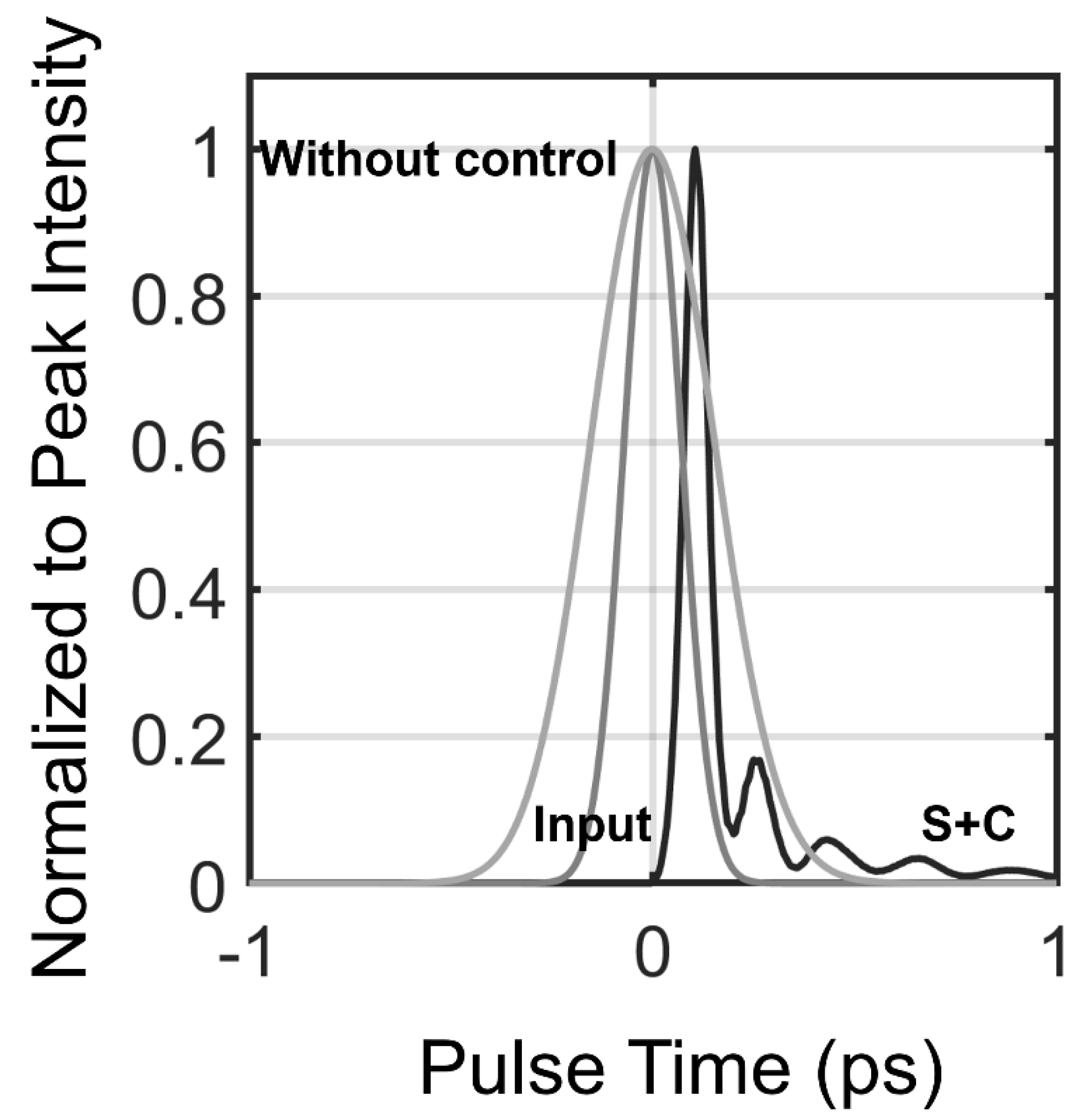
When the control pulse also undergoes significant dispersive effects, i.e., comparable or equivalent to what the signal sees, the ability for it to prevent dispersive broadening for the signal is lowered. In this fiber case, the control pulse sees the same GVD as that of the signal pulse, thus dispersive effects for the control pulse are significant. Figure 2d indicates the results of the propagation of control and signal over 10 m of fiber and compares to the case where the control pulse is not present. It is found that, under the effects of dispersion, the control pulse can still prevent significant signal pulse temporal broadening up to 10 m. At 10 m of propagation, the signal pulse broadens to a factor of 1.8, versus a factor of 19 of temporal broadening when the signal propagates without control. Therefore, the dispersion length of the signal is increased by approximately a factor of 10 when the control pulse is present. The control pulse used for this simulation is the same as the one displayed in Figure 2b, with an overall energy of 800 pJ.
While temporal broadening is prevented, the signal pulse suffers from modulations on its amplitude profile due to distortions of the control pulse’s amplitude profile from dispersion. The control pulse has a dip to zero at the center, as shown in Figure 2b. Under dispersion and self-phase modulation, the two peaks broaden into the dip, resulting in the dip depth being lowered and the slope of the dip being increased (until approximately 1 m of propagation) and then decreased. The dip dynamics of the control pulse then has the result that the signal pulse temporally narrows in duration from the input duration, which is advantageous for certain applications, and then slowly broadens to the duration seen in Figure 2d. Furthermore, because of the high third-order dispersion, the control pulse undergoes an asymmetric broadening of its profile, resulting in the dip becoming asymmetric at the center. The asymmetry in the control pulse results in Airy like side-lobs in the signal pulse, as well as a global shift in central wavelength of the signal pulse through cross-phase modulation.
The resultant effect of the central wavelength shift results in a global delay of the signal pulse with control versus the signal without control. We shifted the signal with control pulse back to time zero in relation to the moving frame of reference of the simulation, so that the comparison with input and dispersed signal is clearly visible in Figure 2d. See Appendix A, Figure A1, for the view of the signal with control at 1 m of propagation, where narrowing of the duration is visible, by a factor of approximately 2 at the full-width half max, along with Airy side-lobs and the delay of the signal pulse with control.
By comparing values of the fiber case with the turbulent dispersion medium of Section 3.1, it is found that the general trend for the p-values is that they scale proportionally to the maximum GVD magnitude within the frequency range of interest. The scaling of the p-values with GVD magnitude is why the control pulse energy in the telecom fiber example (<1 nJ) is significantly lower than the control pulse of the highly fluctuating previous GVD example (i.e., 11 ).
The results of the numerical experiment illustrated in Figure 2d indicate that an ultrafast low-energy pulse can be prevented from substantial temporal broadening up to meters of length in significant normally dispersive fiber. The results are based on the parameters of a popular telecom fiber for 1550 nm radiation used in telecommunications. A practical application is, for example, that dispersive broadening, which would limit fiber links for single-photon experiments in the telecom region, between different labs at a university, can now be utilized with the presence of a control pulse using the method in this paper.
In terms of single-photon experiments, the control pulse would need to be filtered out to preserve the noise floor for the single-photons. The polarization extinction required for the control pulse is approximately 100 dB for this fiber system. However, ultrafast nonlinear polarization rotation experiments, switching the polarization state of a photon using a control-pulse, show that the 100 dB isolation is possible in standard single-mode fiber with the use of two cross-polarizers [42].
Furthermore, we found an experiment utilizing another fiber that is compatible with our method, which may increase isolation between control pulse and single-photon signal. The experiment used cross-phase modulation to increase a single-photon spectrum. The group-velocity of a single photon was matched with that of a control pulse for two wavelengths (800 nm, 1.5 ). The large separation allowed for frequency filtering to obtain a low-noise floor. In this experiment, the fiber has a similar dispersion magnitude profile as the Corning Hi1060flex and the control pulse (at 1.5 ) has negligible dispersion; however, only over ~1 m (as opposed to >10 m in the fiber of this example). Thus, the fiber offered by NKT Photonics is also a candidate to control dispersive effects of a single-photon wavepacket with a control pulse through XPM. More details can be found in [43].
4. Discussion
Through the comprehensive numerical examples shown here, we have shown that our method allows for the control of dispersive effects for arbitrary ultrafast low-energy signal pulses. The waveguide dispersion could be highly fluctuating—for example, around resonances or in practical telecom systems where the bit-rate can now be substantially increased, past the GHz range, limited by the duration of the control pulse. In these examples, the control pulses would enable an upper bound of THz rep-rates, as dispersive effects are not dominant with the control pulse. We also foresee that our method can be used for ultrafast switching, where the dispersion is effectively turned on or off.
This paper so far derives a method to obtain a control pulse that minimizes dispersive effects in a signal pulse through cross phase modulation; however, practically obtaining the said control pulse is not considered up to this point. We then dedicate a portion of the outlook to discuss the generation of the control pulse. The control pulse is not limited to low-energy constraints, and can thus be generated by a wide variety of conventional (lossy) wave-shaping setups.
A popular avenue for ultrafast pulse shaping is to do it in the frequency domain via dynamic diffraction gratings that can modulate the amplitude (and phase) of the spectral profile. These gratings are usually generated through an acousto-optic modulation (AOM) effect found by sending radio-frequency electromagnetic radiation through a piezo-electric medium, surrounding an optically active crystal. The dynamic control of the RF signal induces a desired standing acoustic wave pattern in the crystal, which then acts as a diffractive grating for the optical signal. The scheme ultimately enables the spectral profile of picoseconds down to tens of femtoseconds pulses to be shaped arbitrarily. Extensive literature has explored this subject and there are a plethora of products available to shape ultrafast pulses (with spectral bandwidths even exceeding 50 nm) [44,45,46]. Then, this example scheme should be sufficient to generate the types of control pulses seen in this paper from a seed pulse (e.g., from a Ti/Sa mode-locked laser or an Erbium-doped fiber laser).
Other interesting applications emerge if the amplitude of the control-pulse, whose shape is determined by Equation (4), is increased. Instead of just compensating for temporal broadening, the control-pulse acts to nonlinearly compress the signal-pulse, even in dispersive media where temporal self-compression, for example, due to self-phase modulation, is unlikely, i.e., in normal dispersion.
Our calculations indicate that XPM on a signal-pulse can enhance the spectral broadening (e.g., in normal dispersion waveguides) by a factor of . The temporal compression factor (e.g., in anomalous dispersion waveguides) is also enhanced by the same factor—simply due to this factor of two in the XPM nonlinear coefficient. Thus, using the control-pulse to induce spectral generation through XPM is potentially a highly efficient nonlinear process.
We preliminarily find that simply increasing the amplitude of the found control-pulse from the calculated value given by Equation (4) can induce nonlinear compression of the signal-pulse through the induced additive phase from cross-phase modulation. Thus, the presented method can be used to calculate ideal profiles of control-pulses for XPM on signal-pulses, for the control of such effects as temporal broadening. Furthermore, the method presented here could enhance nonlinear bandwidth generation and nonlinear pulse compression in weak amplitude signals.
Supplementary Materials
The following are available online at https://www.mdpi.com/article/10.3390/photonics8120570/s1, Video S1, the maintained duration and shape of the signal-pulse with control.
Funding
This research received no external funding.
Institutional Review Board Statement
The study did not involve animals.
Informed Consent Statement
The study did not involve humans.
Data Availability Statement
The data are available upon reasonable request to the author.
Acknowledgments
The author would like to thank Pepijn WH Pinkse, Jelmer Jan Renema, and Klaus-J. Boller for helpful discussions on the uses of the method.
Conflicts of Interest
The author declares no conflict of interest.
Appendix A. Wavelength Shift of Signal Pulse and Other Effects on Signal Pulse from Waveform Distortion of the Control Pulse
The position-dependent shift in central wavelength of the signal pulse, as discussed in Section 3.2, is shown as a global delay in the co-moving frame of reference time window of the simulation. As well, the dispersive +SPM effects of the control pulse results in Airy like side-lobs and a narrowing of the pulse duration (non-linear compression) of the signal pulse, through cross-phase modulation. This is indicated in Figure A1 below, showing the pulse development after 1 m of the Gaussian signal pulse of Section 3.2.
Figure A1.
Normalized to peak intensity of the 200 fs Gaussian signal pulse propagated across 1 m of the fiber compared with the input profile and the case without control. Here, the control pulse has full dispersive with SPM effects.
Figure A1.
Normalized to peak intensity of the 200 fs Gaussian signal pulse propagated across 1 m of the fiber compared with the input profile and the case without control. Here, the control pulse has full dispersive with SPM effects.

Appendix B. p-Values for Control Pulses

| Figure Label of Illustrated Signal Pulse | Approx. p-Value (1/m) |
|---|---|
| 1d | 0 |
| 1e | 1.2 × 10³ |
| 1f | 9.8 × 10³ |
| 2b | 0 |
| 2c | 2.0 |
| 2d | 0 |
Figure A2.
(a) Normalized intensity of control pulse, plotted against envelope time in picoseconds, for signal pulse of Figure 1e of Section 3. (b) Normalized intensity of control pulse, plotted against envelope time in picoseconds, for signal pulse of Figure 1f of Section 3. (c) Normalized intensity of control pulse, plotted against envelope time in picoseconds, for signal pulse of Figure 2c of Section 3.

References
- Hasegawa, A.; Tappert, F. Transmission of stationary nonlinear optical pulses in dispersive dielectric fibers. II. Normal dispersion. Appl. Phys. Lett. 1973, 23, 171–172. [Google Scholar] [CrossRef]
- Grahelj, D.; Igor, P. Solitons in Optics; University of Ljubljana: Ljubljana, Slovenia, 2010. [Google Scholar]
- Dudley, J.M.; Genty, G.; Coen, S. Supercontinuum generation in photonic crystal fiber. Rev. Mod. Phys. 2006, 78, 1135–1184. [Google Scholar] [CrossRef]
- Sahin, E.; Blanco-Redondo, A.; Xing, P.; Ng, D.K.T.; Png, C.E.; Tan, D.T.H.; Eggleton, B.J. Bragg Soliton Compression and Fission on CMOS-Compatible Ultra-Silicon-Rich Nitride. Laser Photonics Rev. 2019, 13, 1900114. [Google Scholar] [CrossRef]
- Eggleton, B.J.; de Sterke, C.M.; Slusher, R.E. Nonlinear pulse propagation in Bragg gratings. J. Opt. Soc. Am. B 1997, 14, 2980–2993. [Google Scholar] [CrossRef]
- Liu, Y.; Fu, S.; Malomed, B.A.; Khoo, I.C.; Zhou, J. Ultrafast optical signal processing with Bragg structures. Appl. Sci. 2017, 7, 556. [Google Scholar] [CrossRef]
- Tucker, R.S.; Riding, J.L. Optical Ring-Resonator Random-Access Memories. J. Light. Technol. 2008, 26, 320–328. [Google Scholar] [CrossRef]
- De Goede, M.; Dijkstra, M.; Obregón, R.; Ramón-Azcón, J.; Martínez, E.; Padilla, L.; Mitjans, F.; Garcia-Blanco, S.M. Al2O3 microring resonators for the detection of a cancer biomarker in undiluted urine. Opt. Express 2019, 27, 18508. [Google Scholar] [CrossRef] [PubMed] [Green Version]
- Heideman, R.; Hoekman, M.; Schreuder, E. TriPleX-based integrated optical ring resonators for lab-on-a-chip and environmental detection. IEEE J. Sel. Top. Quantum Electron. 2012, 18, 1583–1596. [Google Scholar] [CrossRef]
- Yebo, N.A.; Taillaert, D.; Roels, J.; Lahem, D.; Debliquy, M.; Van Thourhout, D.; Baets, R. Silicon-on-insulator (SOI) ring resonator-based integrated optical hydrogen sensor. IEEE Photonics Technol. Lett. 2009, 21, 960–962. [Google Scholar] [CrossRef] [Green Version]
- Bogaerts, W.; de Heyn, P.; van Vaerenbergh, T.; de Vos, K.; Kumar Selvaraja, S.; Claes, T.; Dumon, P.; Bienstman, P.; van Thourhout, D.; Baets, R. Silicon microring resonators. Laser Photonics Rev. 2012, 6, 47–73. [Google Scholar] [CrossRef]
- Pittman, T.B.; Franson, J.D. Cyclical quantum memory for photonic qubits. Phys. Rev. A-At. Mol. Opt. Phys. 2002, 66, 4. [Google Scholar] [CrossRef] [Green Version]
- Leung, P.M.; Ralph, T.C. Quantum memory scheme based on optical fibers and cavities. Phys. Rev. A-At. Mol. Opt. Phys. 2006, 74, 1–6. [Google Scholar] [CrossRef] [Green Version]
- Vavulin, D.N.; Sukhorukov, A.A. Effect of loss on single photon parametric amplification. Opt. Commun. 2017, 390, 117–122. [Google Scholar] [CrossRef]
- Bonneau, D.; Mendoza, G.J.; O’Brien, J.L.; Thompson, M.G. Effect of loss on multiplexed single-photon sources. New J. Phys. 2015, 17, 1–15. [Google Scholar] [CrossRef]
- Zhang, J.; Fauchet, P.M.; Painter, O.J.; Agrawal, G.P. Nonlinear optical phenomena in silicon waveguides. Opt. Express 2006, 15, 16604–16644. [Google Scholar]
- Uppu, R.; Wolterink, T.A.W.; Tentrup, T.B.H.; Pinkse, P.W.H. Quantum optics of lossy asymmetric beam splitters. Opt. Express 2016, 24, 16440. [Google Scholar] [CrossRef] [PubMed] [Green Version]
- Islam, M.N.; Sucha, G.; Bar-Joseph, I.; Wegener, M.; Gordon, J.P.; Chemla, D.S. Femtosecond distributed soliton spectrum in fibers. J. Opt. Soc. Am. B 2008, 6, 1149. [Google Scholar] [CrossRef]
- Trillo, S.; Wabnitz, S.; Wright, E.M.; Stegeman, G.I. Optical solitary waves induced by cross-phase modulation. Opt. Lett. 1988, 13, 871–873. [Google Scholar] [CrossRef]
- Nishizawa, N.; Goto, T. Characteristics of pulse trapping by use of ultrashort soliton pulses in optical fibers across the zero-dispersion wavelength. Opt. Express 2002, 10, 1151. [Google Scholar] [CrossRef] [PubMed]
- Wang, S.F.; Mussot, A.; Conforti, M.; Zeng, X.L.; Kudlinski, A. Bouncing of a dispersive wave in a solitonic cage. Opt. Lett. 2015, 40, 3320. [Google Scholar] [CrossRef] [PubMed]
- Deng, Z.; Liu, J.; Huang, X.; Zhao, C.; Wang, X. Active control of adiabatic soliton fission by external dispersive wave at optical event horizon. Opt. Express 2017, 25, 28556. [Google Scholar] [CrossRef]
- Wang, S.F.; Mussot, A.; Conforti, M.; Bendahmane, A.; Zeng, X.L.; Kudlinski, A. Optical event horizons from the collision of a soliton and its own dispersive wave. Phys. Rev. A-At. Mol. Opt. Phys. 2015, 92, 1–6. [Google Scholar] [CrossRef] [Green Version]
- Agrawal, G.P. Applications of Nonlinear Fiber Optics; Elsevier: Amsterdam, The Netherlands, 2001. [Google Scholar]
- Zhang, T.R.; Choo, H.R.; Downer, M.C. Phase and group velocity matching for second harmonic generation of femtosecond pulses. Appl. Opt. 1990, 29, 3927. [Google Scholar] [CrossRef] [PubMed]
- Willenberg, B.; Brunner, F.; Phillips, C.R.; Keller, U. High-power picosecond deep-UV source via group velocity matched frequency conversion. Optica 2020, 7, 485. [Google Scholar] [CrossRef]
- Essiambre, R.J.; Mestre, M.A.; Ryf, R.; Gnauck, A.H.; Tkach, R.W.; Chraplyvy, A.R.; Sun, Y.; Jiang, X.; Lingle, R. Experimental observation of inter-modal cross-phase modulation in few-mode fibers. IEEE Photonics Technol. Lett. 2013, 25, 535–538. [Google Scholar] [CrossRef]
- Malomed, B.A.; Mostofi, A.; Chu, P.L. Transformation of a dark soliton into a bright pulse. J. Opt. Soc. Am. B 2000, 17, 507. [Google Scholar] [CrossRef]
- Dong, Y.; Wang, D.; Wang, Y.; Ding, J. Matching group velocity of bright and/or dark solitons via double-dark resonances. Phys. Lett. Sect. A Gen. At. Solid State Phys. 2018, 382, 2006–2012. [Google Scholar] [CrossRef]
- Wu, T.L.; Chao, C.H. A novel ultraflattened dispersion photonic crystal fiber. IEEE Photonics Technol. Lett. 2005, 17, 67–69. [Google Scholar]
- Lee, S.; Ha, W.; Park, J.; Kim, S.; Oh, K. A new design of low-loss and ultra-flat zero dispersion photonic crystal fiber using hollow ring defect. Opt. Commun. 2012, 285, 4082–4087. [Google Scholar] [CrossRef]
- Hilligsøe, K.M.; Andersen, T.V.; Paulsen, H.N.; Nielsen, C.K.; Mølmer, K.; Keiding, S.; Hansen, K.P.; Kristiansen, R.E.; Larsen, J.J. Supercontinuum generation in a photonic crystal fiber with two closely lying zero dispersion wavelengths. OSA Trends Opt. Photonics Ser. 2004, 96 A, 1567–1568. [Google Scholar]
- Westbrook, P.S.; Nicholson, J.W.; Feder, K.S.; Li, Y.; Brown, T. Supercontinuum generation in a fiber grating. Appl. Phys. Lett. 2004, 85, 4600–4602. [Google Scholar] [CrossRef]
- Sollapur, R.; Kartashov, D.; Zürch, M.; Hoffmann, A.; Grigorova, T.; Sauer, G.; Hartung, A.; Schwuchow, A.; Bierlich, J.; Kobelke, J.; et al. Resonance-enhanced multi-octave supercontinuum generation in antiresonant hollow-core fibers. Light Sci. Appl. 2017, 6, e17124. [Google Scholar] [CrossRef] [Green Version]
- Runge, A.F.J.; Qiang, Y.L.; Alexander, T.J.; Rafat, M.Z.; Hudson, D.D.; Blanco-Redondo, A.; de Sterke, C.M. Infinite hierarchy of solitons: Interaction of Kerr nonlinearity with even orders of dispersion. Phys. Rev. Res. 2021, 3, 1–8. [Google Scholar] [CrossRef]
- Michael, L.B.; Ghavami, M.; Kohno, R. Multiple pulse generator for ultra-wideband communication using Hermite polynomial based orthogonal pulses. In Proceedings of the 2002 IEEE Conference on Ultra Wideband Systems and Technologies (IEEE Cat. No.02EX580), Baltimore, MD, USA, 21–23 May 2002; pp. 47–51. [Google Scholar]
- Zia, H. Simulation of white light generation and near light bullets using a novel numerical technique. Commun. Nonlinear Sci. Numer. Simul. 2018, 54, 356–376. [Google Scholar] [CrossRef] [Green Version]
- Steinberg, A.M.; Chiao, R.Y. Dispersionless, highly superluminal propagation in. Phys. Rev. A 1994, 49, 2071–2075. [Google Scholar] [CrossRef] [PubMed]
- Sharping, J.E.; Okawachi, Y.; Gaeta, A.L. Wide bandwidth slow light using a Raman fiber amplifier. Opt. Express 2005, 13, 6092. [Google Scholar] [CrossRef] [PubMed]
- Agrawal, G.P.; Baldeck, P.L.; Alfano, R.R. Optical wave breaking and pulse compression due to cross-phase modulation in optical fibers. Opt. Lett. 1989, 14, 137–139. [Google Scholar] [CrossRef] [PubMed]
- Zia, H. Enhanced pulse compression within sign-alternating dispersion waveguides. Photonics 2021, 8, 50. [Google Scholar] [CrossRef]
- England, D.; Bouchard, F.; Fenwick, K.; Bonsma-Fisher, K.; Zhang, Y.; Bustard, P.J.; Sussman, B.J. Perspectives on all-optical Kerr switching for quantum optical applications. Appl. Phys. Lett. 2021, 119, 160501. [Google Scholar] [CrossRef]
- Matsuda, N. Deterministic reshaping of single-photon spectra using cross-phase modulation. Sci. Adv. 2016, 2, e1501223. [Google Scholar] [CrossRef] [PubMed] [Green Version]
- Tournois, P. Acousto-optic programmable dispersive filter for adaptive compensation of group delay time dispersion in laser systems. Opt. Commun. 1997, 140, 245–249. [Google Scholar] [CrossRef]
- Verluise, F.; Laude, V.; Cheng, Z.; Spielmann, C.; Tournois, P. Amplitude and phase control of ultrashort pulses by use of an acousto-optic programmable dispersive filter: Pulse compression and shaping. Opt. Lett. 2000, 25, 575. [Google Scholar] [CrossRef] [PubMed]
- Fastlite. Dazzler. 2021. Available online: https://fastlite.com/produits/dazzler-ultrafast-pulse-shaper/ (accessed on 6 December 2021).
Figure 1.
(a) Group-velocity dispersion versus angular frequency with signal (s) and control (c) normalized spectral-density-distributions indicated in gray. (b) Frequency-dependent group-delay with signal and control-pulse locations indicated. (c) Amplitude of control-pulse versus pulse time. (d) Normalized-to-input-peak intensity distribution versus pulse-time for Gaussian signal without control, signal with control, and input profile. Inset is a zoom-in around the controlled signal-pulse. (e) Normalized-to-input-peak intensity distribution versus pulse-time for example of pulse with dip in the middle and two-peaks, signal without control, signal with control, and input profile. (f) Normalized-to-input-peak intensity distribution versus pulse-time for example of slanted asymmetric pulse, signal without control, signal with control, and input profile.


Figure 2.
(a) The group-velocity dispersion versus angular frequency. The frequency of the control (c) and signal (s) is marked by a vertical and horizontal arrow to indicate the respective polarization eigenstates. (b) The normalized to peak intensity of the signal in the presence of control pulse (s + c), the input profile, and the signal without control pulse at the end of a 30 m fiber. The left inset indicates the control pulse’s normalized intensity; the right inset is a zoom-in of the input and signal. (c) Normalized to peak intensity for two pulse shapes chosen ad hoc (signal in black, input profile in dotted gray). (d) Normalized to peak intensity of the 200 fs Gaussian signal pulse propagated across 10 m of the fiber compared with the input profile and the case without control. Here, the control pulse has full dispersive effects with self-phase modulation.


Publisher’s Note: MDPI stays neutral with regard to jurisdictional claims in published maps and institutional affiliations. |
© 2021 by the author. Licensee MDPI, Basel, Switzerland. This article is an open access article distributed under the terms and conditions of the Creative Commons Attribution (CC BY) license (https://creativecommons.org/licenses/by/4.0/).
Share and Cite
MDPI and ACS Style
Zia, H. Maintaining Constant Pulse-Duration in Highly Dispersive Media Using Nonlinear Potentials. Photonics 2021, 8, 570. https://doi.org/10.3390/photonics8120570
AMA Style
Zia H. Maintaining Constant Pulse-Duration in Highly Dispersive Media Using Nonlinear Potentials. Photonics. 2021; 8(12):570. https://doi.org/10.3390/photonics8120570
Chicago/Turabian StyleZia, Haider. 2021. "Maintaining Constant Pulse-Duration in Highly Dispersive Media Using Nonlinear Potentials" Photonics 8, no. 12: 570. https://doi.org/10.3390/photonics8120570
Note that from the first issue of 2016, this journal uses article numbers instead of page numbers. See further details here.