Article

Absolute and Precise Terahertz-Wave Radar Based on an Amplitude-Modulated Resonant-Tunneling-Diode Oscillator

Tokyo Institute of Technology, Meguro, Tokyo 152-8552, Japan
*
Author to whom correspondence should be addressed.
Photonics 2018, 5(4), 52; https://doi.org/10.3390/photonics5040052
Submission received: 29 October 2018 / Revised: 22 November 2018 / Accepted: 23 November 2018 / Published: 27 November 2018
(This article belongs to the Special Issue Terahertz Photonics)

Abstract

:
We present the principle of a terahertz-wave radar and its proof-of-concept experimental verification. The radar is based on a 522 GHz resonant-tunneling-diode oscillator, whose terahertz output power can be easily modulated by superimposing the modulation signal on its bias voltage. By using one modulation frequency and measuring the time delay of the returning signal, a relative measurement of the propagation distance is possible; adding a second modulation frequency removes the ambiguity stemming from the periodicity of the modulation sine wave and allows an absolute distance measurement. We verified this measurement method experimentally and obtained a submillimeter precision, as predicted by theory.

1. Introduction

The terahertz radiation, defined as electromagnetic waves with frequencies roughly between 0.1 and 10 THz (corresponding to wavelengths from 3 mm down to 30 µm), has already started solving real-life problems in fields such as security, safety, and product inspection. This is due to the ability of the terahertz radiation to pass through many visually-opaque materials—textiles, paper, plastics, etc.—while providing sufficient resolution in imaging as well as unique spectral fingerprinting opportunities for material identification [1,2].
From a practical perspective, while in research environments size, complexity, energy consumption, and equipment price are lesser problems, for a commercially successful application of the terahertz waves it is often critical that systems are compact, economic, robust, and inexpensive. In this context, the resonant-tunneling diode (RTD) is a terahertz-wave source on a chip [3], with a size much below one cubic millimeter, working at room temperature, and as such is expected to find its way in future terahertz applications. It only requires a DC bias voltage in the order of 1 V and consumes less than 100 mA to produce a coherent, continuous terahertz wave with a frequency determined by its fabrication parameters (although the frequency can be adjusted to some extent by changing the biasing voltage) and with an output power currently just below the milliwatt order [4,5].
Terahertz imaging provides two-dimensional information on the spatial distribution of a target’s transparency or reflectivity. However, three-dimensional information is often needed, where the additional depth or range dimension allows for the full geometric shape of the target to be reconstructed, upon which decisions can be made. In a product inspection scenario, for instance, three-dimensional measurement of the target may reveal whether or not dents, swellings, or other deformations in a surface are within specifications.
For such cases, a terahertz-wave radar functionality is useful. Currently there are several terahertz technologies providing axial distance measurement. Terahertz time-domain spectroscopy techniques [6] provide excellent ranging resolution, in the order of tens of micrometers, at the cost, however, of a bulky and expensive system that includes a femtosecond pulsed laser and complex optical delays. Frequency-modulated continuous-wave (FMCW) radars in the terahertz range [7,8] are applicable in practice and have started to become commercially available, but only provide resolutions above several millimeters, which is limited by the frequency tunability of the terahertz-wave source; the distance measurement jitter of an FMCW radar can be extremely small, with a standard deviation below 1 µm having been demonstrated for a SiGe radar that allows very precise ranging at a frequency around 240 GHz [9]. Interferometric methods are able to detect distance variations much below the wavelength, but have the drawback of only providing relative distance measurements, unless a multiwavelength approach is taken, such as in a previous paper [10], where two terahertz-wave sources were used.
Here we propose a new ranging method that relies on the principle of the amplitude-modulated continuous-wave (AMCW) radar [11] and benefits from the RTD’s ability to be easily modulated in power. Unlike a usual AMCW radar, which has a ranging ambiguity equal to half the wavelength of the modulation frequency, our method combines phase measurements at two modulation frequencies, in a multiwavelength approach that is different from the one cited above, allowing us to measure the propagation distance both absolutely and accurately, down to a submillimeter uncertainty. The ambiguity range is not just extended to a longer, synthetic wavelength, as it is usual in two-wavelength interferometry, but unlimited. To our knowledge, this is the first report of its kind.
In a previous stage of this research [12], only one modulation frequency was used, which meant the measured distance was relative to some arbitrary starting point. Propagation distances changing by more than one wavelength could only be measured by following the phase evolution in the case of a continuously changing distance. An absolute measurement of the distance was not possible; this report solves that limitation. In addition, the ranging error reported here is about an order of magnitude better.

2. Principle

The radar method we propose relies on using the terahertz wave as a carrier for a lower frequency sinusoidal signal that modulates the amplitude of the carrier. By analyzing the phase delays in the demodulated echo signal, information can be extracted about the propagation time.
For the purpose of illustrating the principle, the block diagram of a propagation length measurement system is shown in Figure 1a. While not having a typical radar configuration, with an echo beam reflecting off a target, this setup allows the verification of the distance measurement principle and we used it in our initial experiments.
The distance measurement presented here is a two-step procedure, detailed in the following subsections. In the first step, phase delays measured at two modulation frequencies are used to determine a rough, but absolute, value of the propagation time difference. This absolute value then is used in the second step, where a more precise value is obtained from the time delay measured at one modulation frequency.

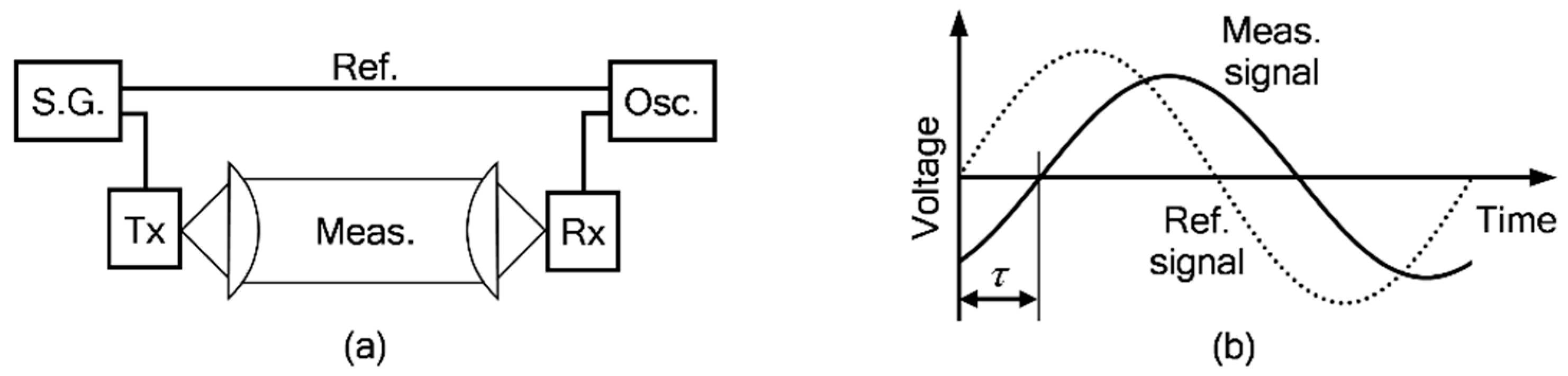
2.1. Step 1: Absolute Propagation Time Difference

At any modulation frequency f, the signal generator outputs the following voltage.
V SG ( t ) = A SG sin ( 2 π f t ) ,
where ASG is the oscillation amplitude and the oscillation phase is taken as zero.
After being divided into the reference and measurement paths and allowed to propagate up to the oscilloscope, the two recorded signals become
V ref ( t ) = A ref sin ( 2 π f t Φ ref ) ,
V meas ( t ) = A meas sin ( 2 π f t Φ meas ) ,
where symbols V, A, and Φ represent voltage, amplitude, and phase, respectively, with subscripts ref and meas identifying quantities of the reference path and measurement path, respectively. The phase delays Φref and Φmeas consist of phase shifts that are due to propagation delays as well as shifts produced by intervening circuit elements such as the terahertz-wave source, detector, amplifier, etc., denoted by φref and φmeas below.
Φ ref = 2 π f t ref + φ ref ,
Φ meas = 2 π f t meas + φ meas .
Here, tref and tmeas are the propagation times on the reference and measurement paths, respectively, and this derivation seeks to find the difference between them.
The phase difference between the signals is then
Δ Φ = Φ meas Φ ref = 2 π f ( t meas t ref ) + φ meas φ ref .
Unfortunately, the phase difference that can be measured directly in the recorded signals is wrapped, that is, the information on the integer number of 2π periods is lost because of the periodicity of the sine function, and only the remaining fraction, named ΔΦwrapped below, is accessible in the waveform, for instance on an oscilloscope:
Δ Φ wrapped = Δ Φ n 2 π ,
where n is a still unknown integer number of periods; it will be determined in the second step of the procedure.
When ΔΦwrapped is measured at two different modulation frequencies, f and f′, the following equations are obtained.
Δ Φ wrapped ( f ) = 2 π f ( t meas t ref ) + φ meas ( f ) φ ref ( f ) n 2 π ,
Δ Φ wrapped ( f ) = 2 π f ( t meas t ref ) + φ meas ( f ) φ ref ( f ) n 2 π .
The same n appears in the two equations above, which for the measurement has an important consequence: when the modulation frequency is changed from f to f′, the user (or software) must make sure they are following the waveform as it evolves and that the same point on it—for instance, the same zero crossing—is being measured. For that purpose, the modulation frequency must be changed progressively (continuously or in sufficiently small steps), to make sure n does not change. With this precaution, there is in principle no limit to the range of measurable distances. If, however, this precaution is not taken, the method described here will only be valid for a limited range of the propagation time difference; that unambiguous range is inversely proportional to the difference between the modulation frequencies. Since, as will become clear further below, the modulation frequency difference will need to be as large as possible for accuracy reasons, the unambiguous range would be very short, hence the progressive change of the modulation frequency becomes a necessity.
Subtracting Equation (8) from Equation (9) leads to
Δ Φ wrapped ( f ) Δ Φ wrapped ( f ) = 2 π ( f f ) ( t meas t ref ) + φ meas ( f ) φ ref ( f ) φ meas ( f ) + φ ref ( f ) .
The wrapped phase differences are calculated from time delays τ and τ′ measured on the oscilloscope as shown in Figure 1b at the modulation frequencies f and f′, respectively:
Δ Φ wrapped ( f ) = 2 π f τ ,
Δ Φ wrapped ( f ) = 2 π f τ .
Plugging Equations (11) and (12) into Equation (10) and solving for the propagation time difference gives
t meas t ref = f τ f τ φ meas ( f ) φ ref ( f ) φ meas ( f ) + φ ref ( f ) 2 π f f .
The four phase values in Equation (13) can in principle be determined experimentally. However, in this particular combination they represent a difference of differences, namely, how much the phase difference between the reference and the measurement arms changes with the modulation frequency. As such, unless one of the paths includes an element whose phase changes rapidly with the modulation frequency (such as a band-pass filter with a narrow band) and which is not balanced by a similar element in the other path, that part of the formula is usually negligible and can be taken zero. This will lead to a small systematic offset of the calculated absolute distance, normally much smaller than a wavelength of the modulation frequency. If this offset can be neglected, the following simplified formula can be used.
t meas t ref = f τ f τ f f .
The propagation time difference can now be used to calculate the propagation distance difference, taking into account the speed of light, c = 299,792,458 m/s by definition, and the refractive index of the air, nair = 1.0003:
d meas d ref = c n air ( t meas t ref ) .
The distance to the target is then taken as half the propagation distance difference:
d target = c 2 n air ( t meas t ref ) .
The physical meaning of dtarget is that it represents the distance in air between the target and the point in the measurement path where the signal takes the same amount of time to arrive from the signal generator as it takes to propagate through the whole reference path. Depending on the optical and cable configuration, that point may be virtual (not a real point in air); also, if the reference path is long, dtarget may be negative.

2.2. Error Estimation for Step 1

The uncertainty of determining the propagation time difference can be estimated by analyzing Equation (14):
δ ( t meas t ref ) = [ δ ( f τ f f ) ] 2 + [ δ ( f τ f f ) ] 2 .
Since any modern signal generator outputs highly accurate frequencies, at least for the purpose of this work, the uncertainties for the modulation frequency values can be taken exactly zero, such that the only error source is the measurement of the time delays τ and τ′:
δ ( t meas t ref ) = f 2 ( δ τ ) 2 + f 2 ( δ τ ) 2 f f .
If we further assume the time delay uncertainties are equal at both modulation frequencies, the formula can be simplified to
δ ( t meas t ref ) = f 2 + f 2 f f δ τ .
Additionally, for a rough estimation, we can assume that the modulation frequency difference is much smaller than the frequencies themselves, and the following approximation is obtained.
δ ( t meas t ref ) 2 2 f + f f f δ τ .
It follows that the uncertainty of the propagation time difference can be reduced by reducing the time delay measurement uncertainty and by increasing the difference between the two modulation frequencies.
As a numerical example, if the modulation frequencies are set to f = 5.7 GHz and f′ = 5.9 GHz, and the time delays can be measured with an uncertainty of δτ = 1 ps (these are actual values used in one of our early experiments), the uncertainty on the propagation time difference will be of about 40 ps, leading to an uncertainty of measuring the propagation distance of about 12 mm (or 6 mm in target position).

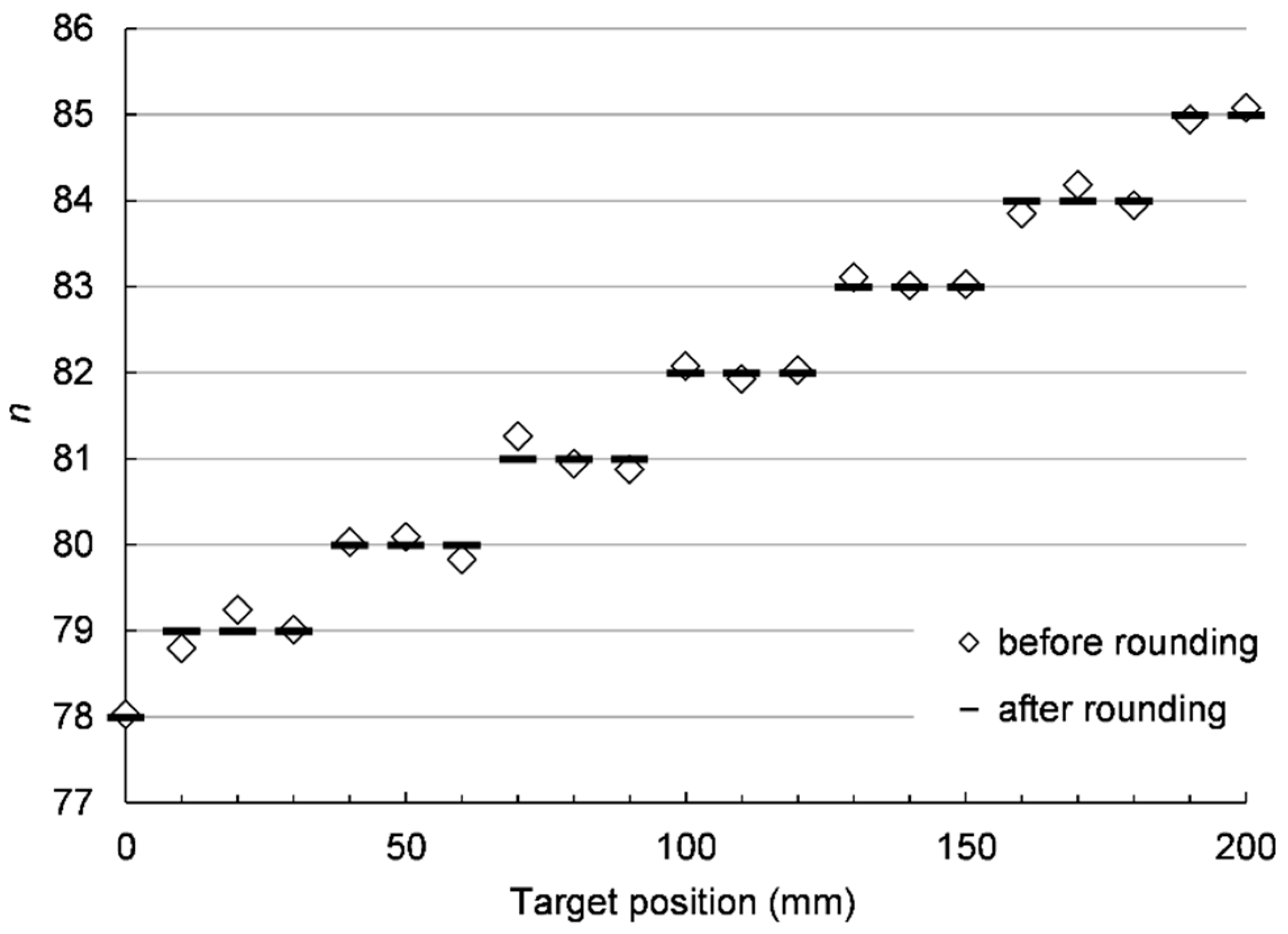
2.3. Step 2: Improved Precision

In the numerical example above, although the time measurement error was taken 1 ps, meaning that propagation distance changes as small as 0.3 mm should be detectable, only distance changes as large as 12 mm can be detected, that is, 40 times worse. This is because, in order to solve the ambiguity arising from the sine wave periodicity, we needed to resort to using a frequency-difference method. But once the ambiguity is solved, it should be possible to use the measured time delays to precisely calculate the propagation time.
Solving the ambiguity means finding n, the unknown number of periods. If we take Equation (8) and in it we plug the newly calculated propagation time difference, for which we will use the simplified version in Equation (14), together with the time–phase relationship given in Equation (11), we arrive at the following result.
2 π f τ = 2 π f f τ f τ f f + φ meas ( f ) φ ref ( f ) n 2 π .
At this point we can extract a formula for n:
n = f f τ f τ f f f τ + φ meas ( f ) φ ref ( f ) 2 π ,
which can be rearranged as
n = f f ( τ τ ) f f + φ meas ( f ) φ ref ( f ) 2 π .
The first term that makes up n accounts for the lengths of cables and optical paths that carry the signal, and increases by 1 for each wavelength (of frequency f) added to the propagation length difference. On the other hand, the second term is usually smaller than 1; while in principle those two phases (or directly their difference) can be determined experimentally, it is easier to give the second term a value between −0.5 and +0.5 such that n becomes an integer. In the case of a set of measurements, such as measuring a series of distances, the term can be fitted so that the calculated values of n are collectively as close to integers as possible; in fact, this amounts to measuring the second term in Equation (23).
If the measurement errors are small enough so that n can be determined with an error that is strictly smaller than 0.5, the ambiguity regarding the number of wavelengths is completely resolved and we can take the value of n obtained in Equation (23) and round it to the closest integer:
n round = [ f f ( τ τ ) f f + φ meas ( f ) φ ref ( f ) 2 π ] ,
where the square brackets represent the operation of rounding.
By ensuring that the uncertainty of n before this rounding operation is strictly smaller than 0.5, the uncertainty of nround is exactly zero; all fluctuations produced by noise have disappeared. With this error-free value of n we can now return to the measurement of the time delay at modulation frequency f (we will not use the measurement at f′) and replace n in Equation (8) with nround:
Δ Φ wrapped ( f ) = 2 π f ( t meas t ref ) + φ meas ( f ) φ ref ( f ) n round 2 π .
Using Equation (11) and rearranging the terms in the equation above, we obtain the following result for the propagation time difference:
t meas t ref = τ + n round φ meas φ ref 2 π f .
The new formula provides a much improved precision. The uncertainty is only given by the time delay τ, since in comparison f can be considered to be known with infinite precision, whereas the error for nround is exactly zero; the phase difference at the numerator can be determined by fitting as explained below Equation (23) and can only affect the result by a systematic amount. Using the same numerical example as above, specifically δτ = 1 ps, the uncertainty of measuring the propagation distance is now reduced drastically, from 12 mm to 0.3 mm.

3. Verification

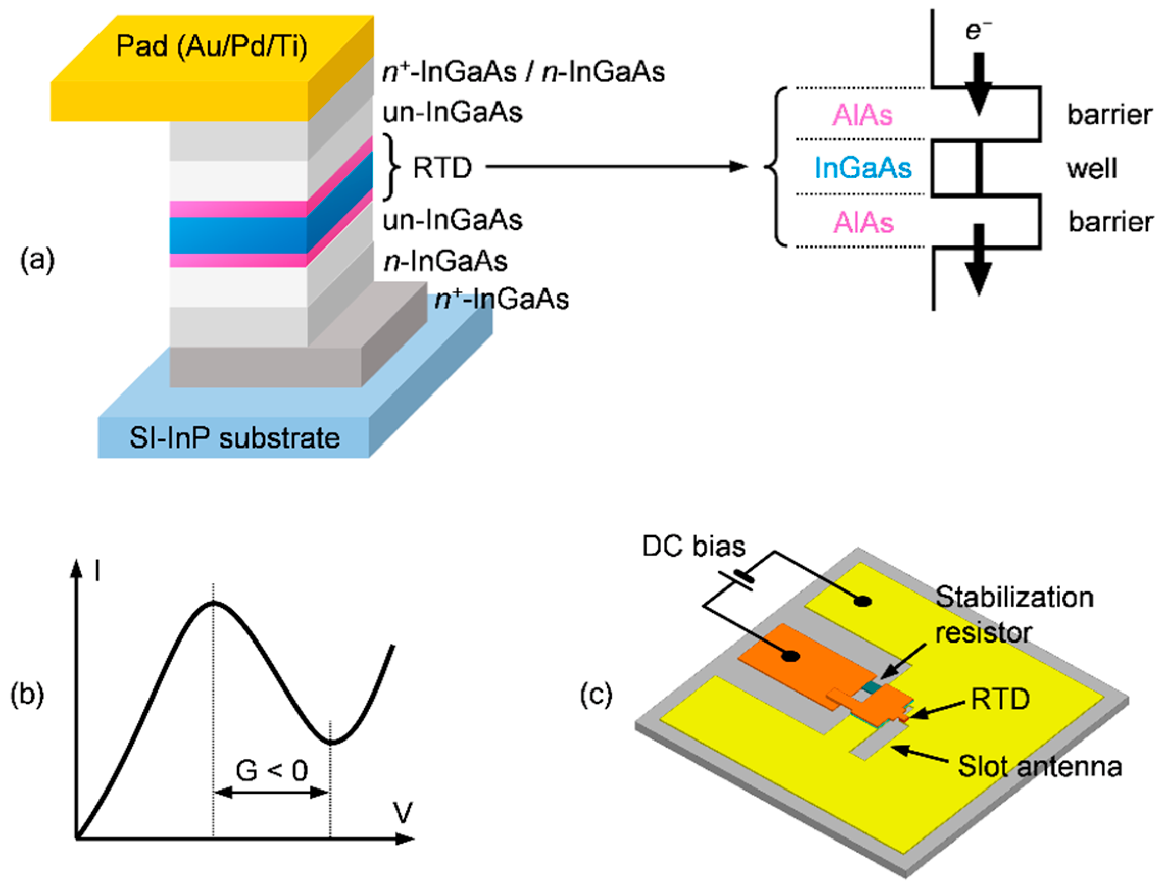
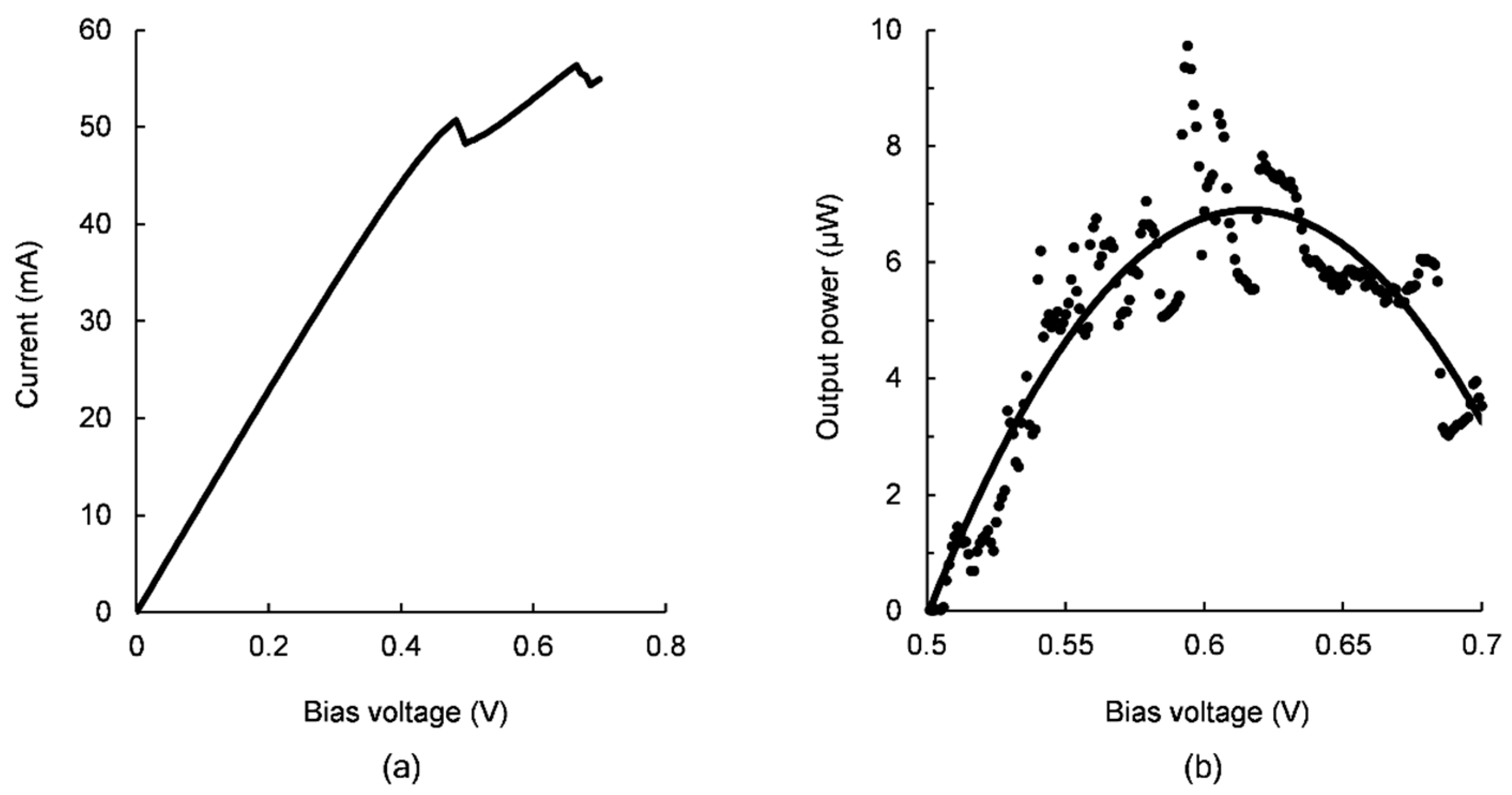
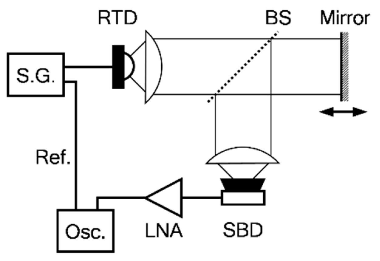
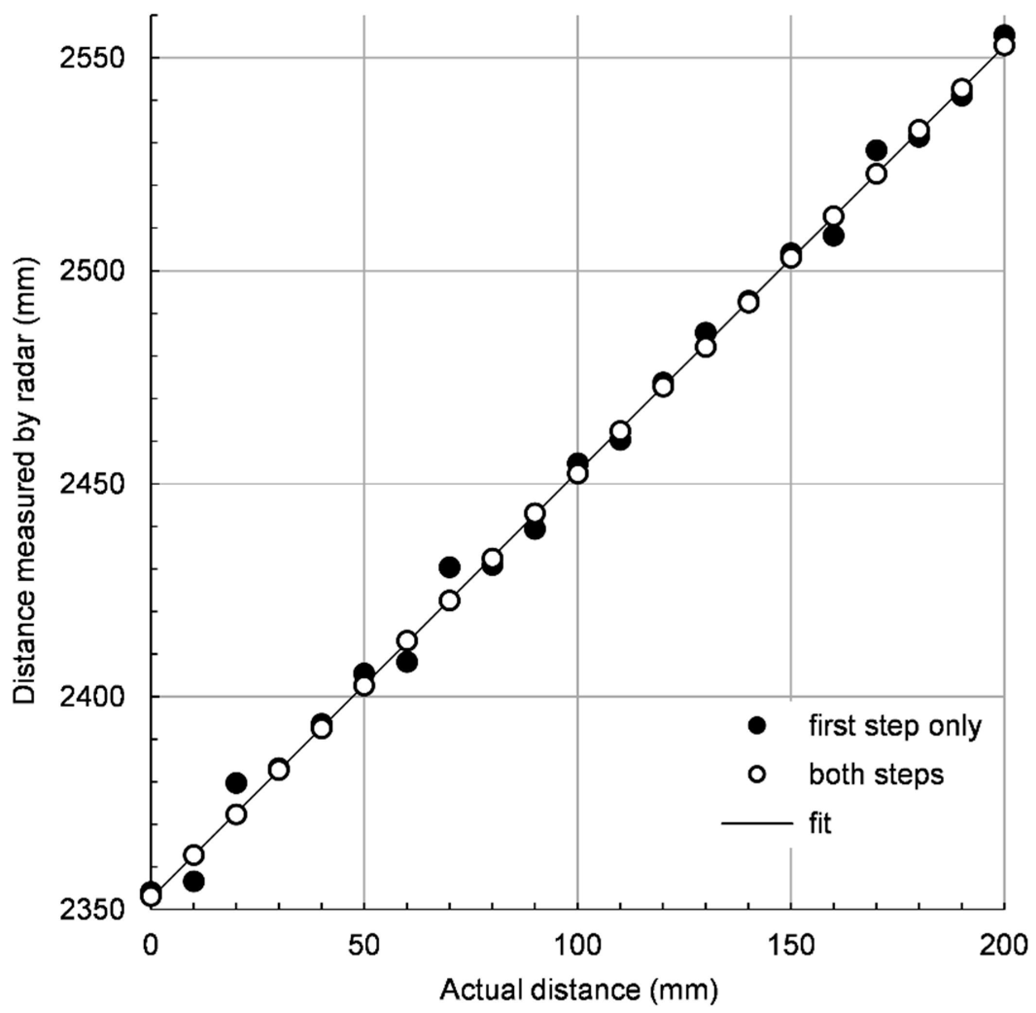
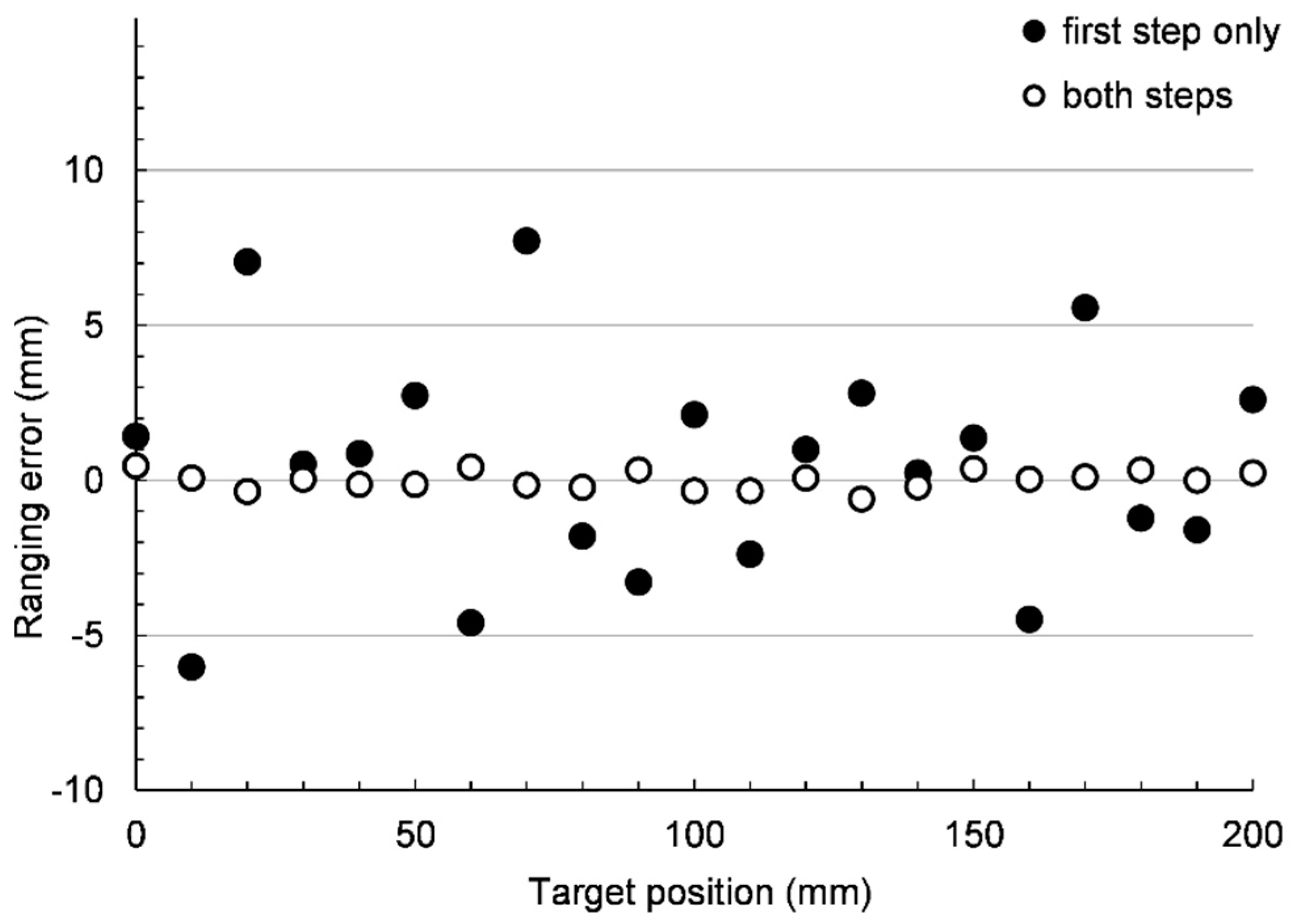
3.1. Experimental Setup

To verify the method experimentally, we used an RTD oscillator fabricated in our lab as a terahertz-wave source, emitting about 10 µW of power at a frequency of 522 GHz, with the structure shown in Figure 2. The RTD is realized as a heterostructure composed of an InGaAs well layer sandwiched between two AlAs barrier layers; additional external layers ensure connectivity. When biased, this structure shows a resonance peak in its current–voltage (I–V) curve, beyond which there is an interval of negative differential conductance (NDC). When the RTD structure is placed in a circuit containing induction and capacity elements and biased in the NDC interval, the circuit starts oscillating; this oscillation is radiated by a slot antenna into the substrate. The substrate is glued to a hyper-hemispherical high-resistivity silicon lens (not shown in the figure), which gives the terahertz radiation the shape of a conical beam when it is released into the free space.
Figure 3 shows the measured I–V curve of the specific RTD used in the radar experiment. The relationship between the bias voltage and the output power is also shown; there is a particular bias voltage on the rising slope, below the maximum power point, at which the RTD emits the strongest amplitude-modulated signal.
For the radar measurements we built the setup shown schematically in Figure 4. The output of a signal generator is divided into a reference that goes directly to the oscilloscope and a signal that modulates the RTD emission power. The terahertz beam from the RTD is first collimated using a plastic lens and passed through a beamsplitter, which is a thin plate of high-resistivity silicon. The beam then reflects off a gold-coated mirror playing the role of target for this radar system; the mirror is placed on a motor stage (with a positioning error below 15 µm and a movement range of 200 mm) so that the distance being measured by the radar can be adjusted. Part of the beam returning to the beamsplitter is reflected and another plastic lens focuses it on the receiver. The collimated beam diameter is limited by the 30 mm aperture of the lenses and the total length of propagation in air is about 1 m.
The receiver is a commercial Schottky-barrier-diode (SBD) detector (model WR1.9ZBD produced by Virginia Diodes, Inc., Charlottesville, VA, USA). The detected signal is amplified with a low-noise amplifier (LNA) up to a level of approximately −15 dBm and fed to the oscilloscope (Keysight DSA91304A Infiniium, with a bandwidth of 13 GHz) as the measurement signal. For the sake of simplicity, other circuit elements—a power divider, bias tees, a circulator, and various power supplies—are not shown in the figure.
It should be noted that adding a sinusoidal signal to the RTD bias voltage does not only modulate its output power, but to some extent also its oscillation frequency. However, this does not affect the results presented here, since the carrier frequency does not play a significant role in measuring the distance.
The relationship between current and output power in the RTD is nonlinear and generates harmonics of the modulation frequency, and the nonlinearity of the SBD detector adds harmonics of its own. We removed these harmonics in the oscilloscope by applying a digital low-pass filter with a cut-off below twice the lowest modulation frequency (8 GHz). This filtering is critical in reducing the errors of the phase measurements.
Since terahertz ranging in humid air may suffer from strong absorption in water vapor, we chose our 522 GHz carrier frequency sufficiently far from the stronger absorption lines in the terahertz range, such as the 557 GHz or the 752 GHz water lines. While in our case the total propagation distance in air was only about 1 m, terahertz-wave radar measurements at distances up to 25 m have been demonstrated at 675 GHz [7].

3.2. Measurement Results

We performed several series of experiments with various optical and electronic configurations, and signal parameters. After progressive improvements, we obtained the result described below.
In order to determine the value of n with a sufficiently small uncertainty (strictly below 0.5), the modulation frequencies were chosen to be 5 GHz and 6 GHz; for reference, the corresponding wavelengths in air are about 60 mm and 50 mm, respectively. Additionally, the waveforms collected by the oscilloscope needed to be averaged 1024 times; with this amount of waveform averaging, we estimated through repeatability tests that the uncertainty of time delay measurements is in the order of a few picoseconds, which should lead to a ranging uncertainty below 1 mm after the second calculation step.
The mirror acting as target object for the radar was moved in 10 mm increments over a distance of 200 mm. At each position, the algorithm detailed in the “Principle” section above was applied and the distance to the target was determined.
Figure 5 shows the absolute distance measured by the radar versus the actual (but relative) position of the target. A linear fit, whose slope was forced to be exactly 1, is also shown. For more clarity, Figure 6 plots the errors relative to the linear fit. To illustrate the importance of applying the second step of the algorithm, the intermediate results obtained when using only the first step were added to both figures. The improvement is obvious: while after the first step the error is up to 8 mm, performing the second step reduces the error by one order of magnitude, to about 0.6 mm.
The absolute quality of the measurement is seen in the intercept of the fitting line in Figure 5. Its value of 2352.7 mm represents half the propagation length difference between the measurement and the reference paths when the motor stage holding the mirror is placed at its zero position. Changing the cable lengths in the circuit leads to changes in the intercept value; cable lengths are shorter than the calculated propagation lengths, however, as the speed of signals through them is about 0.7 of the speed of light in the air.
As mentioned in the “Principle” section, this significant reduction of the error is due to the rounding operation on the number n. Figure 7 shows a plot of the unrounded values of n. The steps have an increment of 1 and a length of 30 mm, which is half the wavelength at 5 GHz. The errors before rounding are at most 0.25, safely below the 0.5 limit, beyond which the errors would propagate through the rounding operation, compromising the measured distance.

3.3. Improvement Ideas

In some applications, such as radars used in automobiles for collision avoidance, the accuracy level after the first algorithm step is already good enough, and the error can be further reduced by choosing two modulation frequencies that are further away from each other. However, this way of improving the accuracy is limited by the maximum frequency of the signal generator and of the signal processing, as well as by the RTD itself, whose modulation capability deteriorates above 10 GHz, but can, with special precautions, be increased up to about 30 GHz [13].
The error after the second step cannot be further reduced by choosing more distant modulation frequencies, since this uncertainty is given only by the error of measuring time delays. The accuracy can be improved, however, by increasing the power of the modulated terahertz signal arriving at the SBD. In a separate experiment, where the SBD was placed directly in front of the RTD (each with its corresponding lens), such that the losses in the beamsplitter were removed, the stronger signals led to an accuracy of 0.4 mm.
We expect that if we automate the time delay measurements—by reading the waveforms into a computer and fitting them with sinusoids—we can further improve the ranging accuracy of the radar, since the whole waveform would contribute to the measurement rather than using only the small portion near a zero crossing as we do now.
Automation may even allow us to apply two or more amplitude modulation signals simultaneously, in which case the time delays would be determined through signal processing, by fitting the demodulated waveform with a sum of sinusoids. This would have the advantage of a shorter measurement time, which would be particularly useful when long series of measurements are performed.
In our proof-of-concept experiment we used an oscilloscope to measure phase delays, but in an actual application this would be impractical and expensive. We are already working on replacing the oscilloscope with a quadrature demodulation circuit, in which the phase is determined by the homodyne mixing of the return signal with a pair of 90° shifted local oscillator signals, in effect building a lock-in amplifier that works at our high modulation frequencies. With careful error correction, we hope to obtain a better ranging resolution than with the oscilloscope.

4. Conclusions

To our knowledge, this is the first time distances have been measured both absolutely and with submillimeter accuracy using terahertz waves produced by a one-chip semiconductor source.
We are considering using this radar in a three-dimensional reflection imaging experiment, in which case the terahertz beam would be focused on the target. Whereas the same depth resolution as reported here can probably be obtained with electromagnetic waves of lower frequencies, in the microwaves or millimeter waves, the lateral resolution is limited by the carrier wavelength, which is where the terahertz radiation has a strong advantage. At the carrier frequency of 522 GHz we expect the lateral resolution to be below 1 mm, just like the axial resolution. Moreover, among the various room-temperature high-frequency electron devices, RTD’s offer the highest oscillation frequency, with the record being close to 2 THz [14], which gives us a wide choice of radar carrier frequencies.
With a terahertz body scanner application in mind, we are also looking at ways of simultaneously measuring the distances to several semitransparent targets placed in front of a reflecting target, such as layers of clothing in front of the skin or a concealed object.
We have not considered the case of a moving target, either theoretically or experimentally. We expect that at least two effects will occur: (1) the Doppler effect will expand or compress the sine waves, changing their frequencies, which means we need to rethink the signal processing, and (2) if the signals are recorded in sequence at different times for each modulation frequency, the target moving during the measurement will affect the final result.
The same ranging principle as described here can also be applied in other electromagnetic (or sound) wave frequency ranges where sources can be amplitude-modulated. Moreover, if the source frequency can be tuned, such as with microwave or ultrasound sources, the same principle can be used with unmodulated waves, by tuning the source from one frequency to another and measuring the phase delays by homodyne mixing or by using an interferometric setup. In fact, the RTD frequency tunability feature means that we could apply the same method without amplitude modulation, just by adjusting the biasing point; in practice, however, we found that even a weak beam returning into the RTD strongly perturbs the oscillation frequency [15,16], hence a good optical isolation needs to be achieved before radar measurements can be attempted using direct tuning of the RTD frequency.

Author Contributions

Conceptualization, S.S., M.A., and A.D.; Methodology, A.D.; Formal Analysis, A.D. and R.W.; Investigation, R.W. and Y.S.; Writing—Original draft preparation, A.D.; Writing—Review and editing, M.A. and A.D.; Project Administration, M.A. and S.S.; Funding Acquisition, M.A. and S.S.

Funding

This research was funded by JSPS (16H06292), JST-ACCEL (JPMJMI17F2), JST-CREST (JPMJCR1534), JST Industry-Academia Collaborative R&D, and a SCOPE program of the Ministry of Internal Affairs and Communications (#175003003).

Conflicts of Interest

The authors declare no conflicts of interest.

References

  1. Dobroiu, A.; Otani, C.; Kawase, K. Terahertz-wave sources and imaging applications. Meas. Sci. Technol. 2006, 17, R161–R174. [Google Scholar] [CrossRef]
  2. Song, H.-J.; Nagatsuma, T. Handbook of Terahertz Technologies: Devices and Applications; Pan Stanford Publishing: Singapore, 2015; ISBN 978-981-4613-08-8. [Google Scholar]
  3. Asada, M.; Suzuki, S. Resonant tunneling diodes for terahertz sources. In Handbook of Terahertz Technologies: Devices and Applications; Song, H.-J., Nagatsuma, T., Eds.; Pan Stanford Publishing: Singapore, 2015; pp. 151–185. ISBN 978-981-4613-08-8. [Google Scholar]
  4. Suzuki, S.; Shiraishi, M.; Shibayama, H.; Asada, M. High-power operation of terahertz oscillators with resonant tunneling diodes using impedance-matched antennas and array configuration. IEEE J. Sel. Top. Quantum Electron. 2013, 19, 8500108. [Google Scholar] [CrossRef]
  5. Kasagi, K.; Suzuki, S.; Asada, M. Large-element array of resonant-tunneling-diode terahertz oscillator for high output power at 1 THz region. In Proceedings of the Compound Semiconductor Week (CSW2018), Cambridge, MA, USA, 29 May–1 June 2018. [Google Scholar]
  6. Nuss, M.C.; Orenstein, J. Terahertz time-domain spectroscopy. In Millimeter and Submillimeter Wave Spectroscopy of Solids; Grüner, G., Ed.; Springer: Berlin/Heidelberg, Germany, 1998; ISBN 978-3-662-30953-7. [Google Scholar]
  7. Cooper, K.B.; Dengler, R.J.; Llombart, N.; Thomas, B.; Chattopadhyay, G.; Siegel, P.S. THz imaging radar for standoff personnel screening. IEEE Trans. Terahertz Sci. Technol. 2011, 1, 169–182. [Google Scholar] [CrossRef]
  8. Caris, M.; Stanko, S.; Wahlen, A.; Sommer, R.; Wilcke, J.; Pohl, N.; Leuther, A.; Tessman, A. Very high resolution radar at 300 GHz. In Proceedings of the 44th European Microwave Conference, Rome, Italy, 6–9 October 2014; pp. 1797–1799. [Google Scholar]
  9. Jaeschke, T.; Bredendiek, C.; Pohl, N. A 240 GHz ultra-wideband FMCW radar system with on-chip antennas for high resolution radar imaging. In Proceedings of the 2013 IEEE MTT-S International Microwave Symposium Digest, Seattle, WA, USA, 2–7 June 2013. [Google Scholar] [CrossRef]
  10. Wang, X.; Hou, L.; Zhang, Y. Continuous-wave terahertz interferometry with multiwavelength phase unwrapping. Appl. Opt. 2010, 49, 5095–5102. [Google Scholar] [CrossRef] [PubMed]
  11. Nilssen, O.K.; Boyer, W.D. Amplitude modulated CW radar. IRE Trans. Aerosp. Navig. Electron. 1962, 4, 250–254. [Google Scholar] [CrossRef]
  12. Hu, J.; Wakasugi, R.; Suzuki, S.; Asada, M. Amplitude-modulated continuous wave ranging system with resonant-tunneling-diode terahertz oscillator. In Proceedings of the 2018 43rd International Conference on Infrared, Millimeter, and Terahertz Waves (IRMMW-THz), Nagoya Aichi, Japan, 9–14 September 2018. [Google Scholar]
  13. Ikeda, Y.; Kitagawa, S.; Okada, K.; Suzuki, S.; Asada, M. Direct intensity modulation of resonant-tunneling-diode terahertz oscillator up to ~30 GHz. IEICE Electron. Express 2015, 12, 20141161. [Google Scholar] [CrossRef]
  14. Izumi, R.; Suzuki, S.; Asada, M. 1.98 THz resonant-tunneling-diode oscillator with reduced conduction loss by thick antenna electrode. In Proceedings of the 2017 42nd International Conference on Infrared, Millimeter, and Terahertz Waves (IRMMW-THz), Quintana Roo, Mexico, 27 August–1 September 2017. [Google Scholar]
  15. Asada, M.; Suzuki, S. Theoretical analysis of external feedback effect on oscillation characteristics of resonant-tunneling-diode terahertz oscillators. Jpn. J. Appl. Phys. 2015, 54, 070309. [Google Scholar] [CrossRef]
  16. Manh, L.D.; Diebold, S.; Nishio, K.; Nishida, Y.; Kim, J.; Mukai, T.; Fujita, M.; Nagatsuma, T. External feedback effect in terahertz resonant tunneling diode oscillators. IEEE Trans. Terahertz Sci. Technol. 2018, 8, 455–464. [Google Scholar] [CrossRef]
Figure 1. (a) Schematic of a propagation time difference measurement setup. S.G. = signal generator. Osc. = oscilloscope. Ref. = cable carrying the reference signal. Meas. = the measurement arm, consisting both of cables and free-space propagation. Tx = transmitter. Rx = receiver. (b) Time delay measurement.
Photonics 05 00052 g001
Figure 2. (a) Resonant-tunneling diode (RTD) layer structure. (b) I–V curve for a typical RTD, showing a biasing interval where the differential conductance is negative. (c) The RTD device containing biasing pads and a slot antenna. The device area is about 1 × 1 mm.
Photonics 05 00052 g002
Figure 3. (a) Measured I–V curve of the RTD chip used for this experiment. The chip includes a stabilization resistor connected in parallel with the RTD, as shown in Figure 2c, which explains the difference from the typical I–V curve around the NDC region. (b) The dependence of the RTD output power on the bias voltage; dots: measured data; solid line: data smoothed to show the average trend. The large fluctuations are due to terahertz radiation coming back to the RTD and affecting its oscillation frequency. The strongest carrier power, almost 10 µW, is obtained at a bias voltage of around 0.60 V, but the amplitude modulation is the most efficient at 0.56 V.
Photonics 05 00052 g003
Figure 4. Schematic of the experimental setup.
Photonics 05 00052 g004
Figure 5. Distance measured by the radar versus actual target displacement distance. After applying the second step of the algorithm, the errors become too small to see in this plot.
Photonics 05 00052 g005
Figure 6. Errors in the distance measurement. The largest deviation after the first step is +7.7 mm (at position 70 mm); after the second step the largest deviation is −0.61 mm (at a position of 130 mm).
Photonics 05 00052 g006
Figure 7. The values of n, before and after rounding.
Photonics 05 00052 g007

