Article

Determining Topological Charge of Bessel-Gaussian Beams Using Modified Mach-Zehnder Interferometer

Department of Physics, Indian Institute of Technology Patna, Bihta, Patna 801106, Bihar, India
*
Author to whom correspondence should be addressed.
Photonics 2024, 11(3), 263; https://doi.org/10.3390/photonics11030263
Submission received: 21 February 2024 / Revised: 7 March 2024 / Accepted: 11 March 2024 / Published: 14 March 2024
(This article belongs to the Special Issue Structured Light Beams: Science and Applications)

Abstract

:
The orbital angular momentum (OAM) associated with structured singular beams carries vital information crucial for studying various properties and applications of light. Determining OAM through the interference of light is an efficient method. The interferogram serves as a valuable tool for analyzing the wavefront of structured beams, especially identifying the order of singularity. In this study, we propose a modified Mach–Zehnder interferometer architecture to effectively determine the topological charge of Bessel–Gaussian (BG) beams. Several numerically generated self-referenced interferograms have been used for analysis. Moreover, this study examines the propagation property and phase distribution within BG beams after they are obstructed by an aperture in the interferometer setup.

1. Introduction

Bessel–Gaussian (BG) beams form a unique type of structured singular beams, well-known for their non-diffracting intensity distribution. If such beams encounter obstacles while traversing, they exhibit a distinctive and intriguing ability of self-healing [1,2,3,4,5,6,7,8,9,10]. The exceptional features imply their potential application across diverse areas like material processing, which involves tasks such as cutting and drilling [11,12,13]. Moreover, BG beams find practical utility in optical communication [14,15], including wireless underwater communication [16]. Their resilience to underwater turbulence caused by temperature and salinity makes them a robust choice for communication in such environments. Also, BG beams contribute significantly to optical tweezers [17] and high-resolution imaging [18]. For the progress of potential applications, various efficient methods for BG beam generation have been reported [19,20,21,22,23,24,25,26,27,28,29,30,31].
In 1987, Durnin discovered that the solution to the free space Helmholtz equation in spherical coordinates carries the zeroth-order Bessel function. The study demonstrated the generation of zero-order BG beams through the use of apertures [32,33]. Later, Arlt and Dholakia reported that the BG beams could be achieved by using an axicon lens. After passing through an axicon lens, the resulting superposition of plane waves inclined at a constant conical angle θ generates BG beams of zero-order [19]. Higher-order BG beams can be achieved by shining Laguerre–Gaussian (LG) beams onto an axicon lens [20]. Further, several methods utilizing computer-generated holograms (CGH) for the generation of BG beams have been reported [21,22]. These approaches utilize axicon holograms encoded onto a spatial light modulator (SLM). For the generation of higher-order BG beams, SLM encoded with a combined spatial phase plate (SPP) and axicon phase-only hologram have been utilized [23,24]. The utilization of metasurfaces has also been reported [25].Fabry–Perot resonator-based BG beam generation has also been reported [26,27].In the resonator, constructive and destructive interferences occur between the standing waves, resulting in a circular, symmetric spatial-frequency spectrum. Efforts have been made to generate BG beams with fiber [28,29]. BG beams produced through fiber-based technology deliver a compact and flexible implementation compared to diffractive optical elements. However, it is challenging to design fiber with a special diffractive structure to generate BG beams [30].
Recently, we demonstrated a dual-modulation-based technique for the generation of BG beams through cascaded phase-only holograms. In this case, both the holograms were designed to precisely modulate the desired amplitude as well as phase within the incoming beam. The generated BG beams with this approach are beneficial in achieving the desired beam in zeroth order with sufficiently high energy as compared to beams produced in first order using grating [30]. Also, there is no limitation on the range of BG beams produced as compared to the case of axicons, which may be an essential requirement in various practical applications.
BG beams are a special class of structured, singular light beams that are spatially varying in amplitude and phase. Hence, their generation requires both modulations within the light beam. The field distribution of BG beams consists of a helical wavefront for higher-order topological charge (TC) values, which depends upon the azimuth phase eilφ where l represents the order of BG beams, also termed the TC, associated with orbital angular momentum (OAM). The TC and OAM are related with a relation of ±lh/2π per photon. Here, h and φ, respectively, denote Planck’s constant and azimuthal angle [34,35,36]. They are generated by the circulation of azimuth phase values around the optical axis of propagation. While at the center, the gradient of phase is zero and, consequently, a dark center is created, which is characterized by an undefined phase resulting in a doughnut-shaped intensity profile. The dark center defined by a singularity in phase is known as a singular point or vortex. The size of the singular point increases as we increase the order of the TC associated with vortex beams. The TC denotes the number of phase revolutions per wavelength around the singular point, which can take any integer value. Zeroth- and higher-order BG beams are found to have bright and dark centers, respectively.
Various studies have been reported for the determination of the vortex charge. Diffraction fields arising from the transmission of a vortex beam through slits [37,38], triangular apertures [39], and various lenses [40,41] have been investigated for TC determination. On the other hand, interferometric techniques provide a more convenient way for TC determination. They involve interference either with the reference beam or with its own amplitude-split copy. Usually, a reference beam, like a Gaussian beam, plane waves, and spherical waves, is utilized for achieving interference. Different interferogram patterns like fork, spiral, and petal fringe patterns, are obtained employing various interferometric techniques, which provide flexibility in determining the magnitude and sign of the TC within vortex beams by simply counting the number of fringes originating at the location of the vortex [42,43,44]. Self-referenced interferometric techniques offer flexibility in the event of the unavailability of the reference beam [45,46].When a vortex beam interferes with its own misaligned copy, a pair of fork-shaped patterns is obtained [47,48,49]. An improved Fizeau interferometer has been used to obtain a self-referenced spiral interferogram, which provides knowledge of the sign and magnitude of the TC of vortex beams [50]. A Mach–Zehnder interferometer (MZI) has been reported for achieving TC measurement. The interferometric arrangement of the MZI was modified with a dove prism to determine higher-order TCs [51]. Counting the number of petal fringe patterns gives the magnitude of the TC, which is half the number of fringes obtained. However, the sign of the TC has not been determined. In order to resolve the issue of sign determination, the MZI architecture was further modified by integrating two MZIs with a dove prism [52]. In a recent study, a modified MZI version was reported for higher-order TC determination of the LG vortex beam along with its sign. In this set-up, the beam whose TC is to be determined is directed into the MZI arrangement, which is split into two orthogonal directions. One of the split copies of beam is laterally displaced and introduced with a tilt in one of the arms of the MZI and then made to interfere with its own split conjugate copy, traversing in another arm. This modified version produced a fork-shaped fringe pattern, and on analyzing the interferogram, both the magnitude and sign of the TC can be determined [53]. The astigmatic lens technique has also been reported for TC measurements of the beam with multiple ring dislocations [54].
It is important to identify the order of the singularity given by the TC and the associated OAM within BG beams. To the best of our knowledge, there is a lack of systematic study on the determination of the TC of BG beams. In order to accomplish this task, our intention is to develop a method for determining phase distribution embedded within BG beams. Interferometry is the most convenient way to realize various properties of light fields. We propose a modified MZI architecture to determine the TC of BG beams. Several numerically generated self-referenced interferograms have been used for analysis. A technique of interference where a beam is superposed with its own amplitude or wavefront split copy is known as self-referenced interferometry. The propagation property and phase distribution within BG beams obstructed by an aperture have also been investigated.
The paper is organized as follows: Section 2 describes the principle of BG beam generation; Section 3 describes the interference of Bessel beams with different reference beams; and Section 4 presents various self-referenced interferometric techniques employing modified MZI. Section 5 discusses the propagation behavior when BG beams are obstructed and carrying out its interferogram utilizing a modified MZI.

2. Theoretical Analysis of BG Beams

Principle of Generation of BG Beams

The schematic diagram for the generation of BG beams is shown in Figure 1. Here, the desired BG beam is produced using dual-pass modulations from the phase-only holograms encoded side-by-side on a single liquid crystal SLM [30]. The SLM screen is divided into two parts, where each half is displayed with a computer-generated hologram (CGH). The CGHs are prepared using MATLAB, which can produce different orders of BG modes. Each CGH encoded onto the SLM consists of PVDsφ1 and φ2. The first phase value distribution (PVD) is designed to enable amplitude modulation in the second PVD plane, which finally helps achieve wavefront shaping. Consequently, the desired BG beams with spatially varying amplitude and wavefront can be achieved by manipulating the phase profiles displayed onto the SLM.
Laser light with a wavelength ~ 532 nm (Cobolt, 150 mW) has been used as the incoming light field. Firstly, the state of the polarization of incoming light is set at 45° with respect to the working direction of the SLM. When the incoming light falls at 45° onto SLM’s first half screen, its intensity becomes modulated with an x-axis distribution as 1 2 A 0 { exp ( i ϕ 1 ( x , y ) ) } while the other component remains unmodulated with a y-axis distribution as 1 2 A 0 . Now, the one-time-modulated light beam is passed through a polarizer, which is oriented at 45° with respect to the x-axis. The field distribution after passing through the polarizer is expressed as
E ( x , y ) = A 0 exp { i ϕ 1 ( x , y ) } 2 × 1 2 + 1 2 A 0 × 1 2 = 1 2 A 0 exp i ϕ 1 x , y + 1
For producing second modulation, the beam is rotated back towards the SLM’s other half screen through a right-angled prism. It is also passed through a half-waveplate oriented such as to bring the rotation within the light from 45° to the SLM’s working direction. After the second-time modulation, the electric field distribution can be expressed as
E ( x , y ) = 1 2 A 0 exp i ϕ 1 x , y + 1 exp i ϕ 2 x , y = A 0 cos ϕ 1 2 exp i ϕ 1 + 2 ϕ 2 2
In Equation (2), the cos term determines the amplitude distribution, while wavefront modulation is determined by ϕ 1 + 2 ϕ 2 2 . Hence, by controlling phase profiles encoded onto the SLM, we can generate BG beams of different orders. The electric field distribution of the l-order BG beam is the exact solution to the free-space Helmholtz wave equation in spherical symmetry. It is expressed as
E B G r , ϕ , z = A l J l k r r exp i l ϕ exp r 2 w 0 2
where Jl(x) is the Bessel function of order l, k is the wave vector, and kr and kz are radial and longitudinal wave vector components, respectively. The amplitude of BG beams at a distance z can be calculated using paraxial approximation by Fresnel integration [53].

3. Interference of BG Beams with Reference Beams

In this section, we discuss the interference of BG beams with different types of reference beams, like Gaussian beams and spherical beams. Here, for the measurement of the TC, different interferograms generated through different configurations, like in-line and off-axis interference between BG and reference beams, have been used.

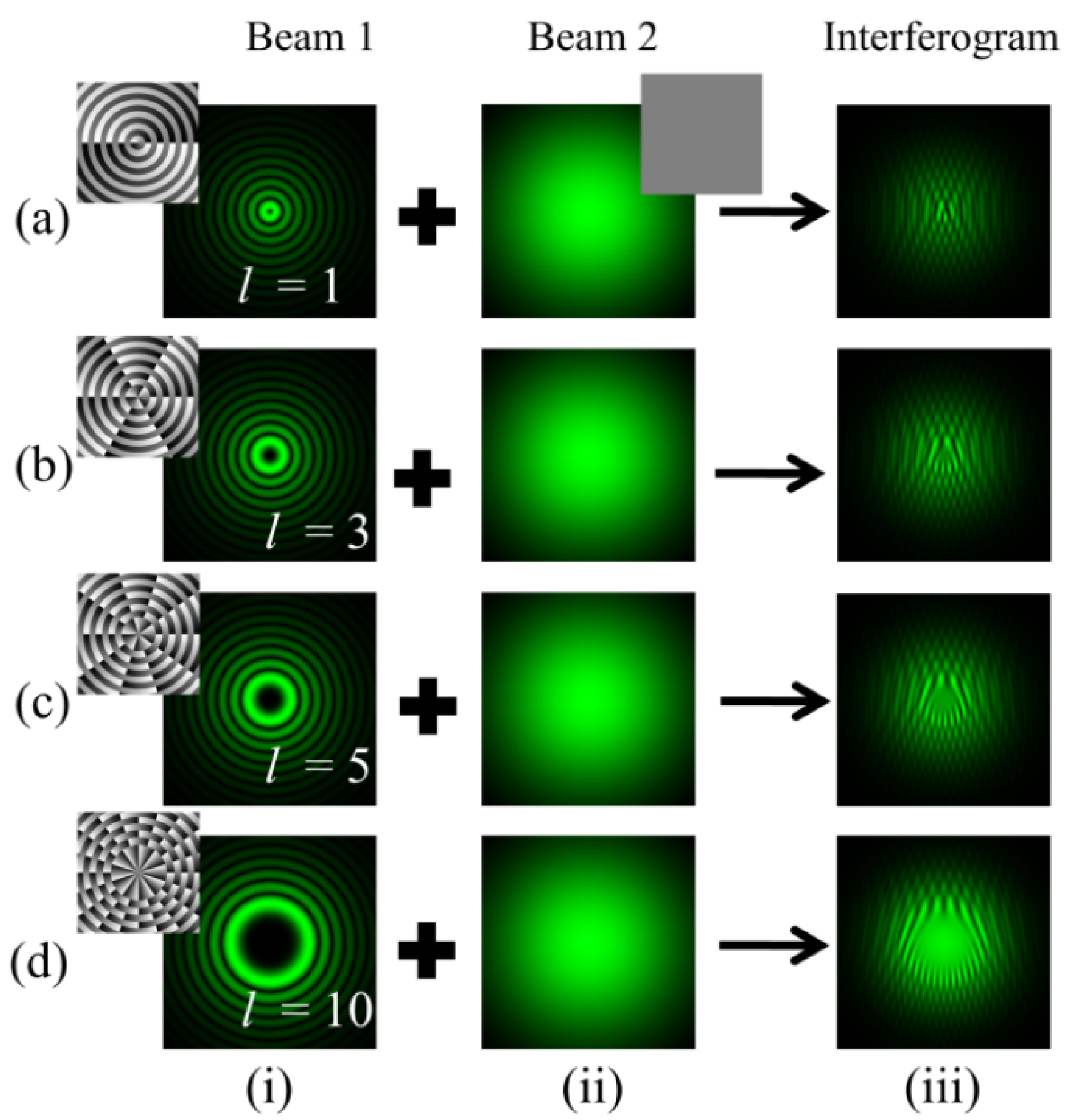
3.1. Bessel Beam Interference with Gaussian Beam

A.
In-line interference
The schematic diagram representing the in-line interference of BG beams with Gaussian beams is shown in Figure 2. The field distribution of a Gaussian beam is described as
E G x , y = A 0 exp r 2 w 0 2
Here, A0, w0, and r denote the amplitude, minimum beam waist, and radius of the incident Gaussian beam, respectively. The interference of BG beams with reference Gaussian beams gives a petal-shaped fringe pattern.
Figure 3 shows the interference pattern obtained after the superposition of BG beams of different orders with the Gaussian beam. The petals are produced at a singular point. Counting the number of petals gives the magnitude of the TC within the BG beam. The intensity distribution of the interference pattern gradually decreases as we move away from the center. The phase profiles corresponding to each order of BG beams are also displayed with their intensity distribution. Column (i) represents the intensity distributions of BG beams of different order l = 1, 3, 5, and 10 as depicted in rows (a–d). Column (ii) describes the intensity distributions of Gaussian beams. Column (iii) represents the obtained intensity distributions of the fringe pattern.
B.
Off-axis interference
In off-axis configuration, the reference beam is subjected to a tilt through a mirror. The tilt function is mathematically expressed as
T x , y = exp i 2 π λ y tan θ
where θ is the tilt angle and λ is the wavelength of light. The reference beam, after introducing a tilt, is expressed as
E G x , y = A 0 exp r 2 w 0 2 T x , y
The off-axis superposition of BG and Gaussian beams is described by the mathematical expression as
E I = E G + E B G l = A 0 exp r 2 w 0 2 exp i 2 π λ y tan θ + A l J l k r r exp i l ϕ exp r 2 w 0 2
The tilt introduced in the reference beam is ~0.2°. The schematic diagram representing the off-axis interference of BG beams with Gaussian beams is shown in Figure 4. The interferogram obtained after the superposition of BG beams of different orders with the tilted Gaussian beam is shown in Figure 5. The obtained patterns consist of fork-shaped fringes, which bifurcate at the wavefront dislocation region. The fringe structure consists of a handle and tines coming out of it. The bright, discontinuous fringes encircling the singular region in the interference fringe pattern provide direct insight into the magnitude of the TC carried by the BG beam. TC is determined by counting the number of tines using the relation |l| = m, where m represents the count of additional discontinuous bright fringes.

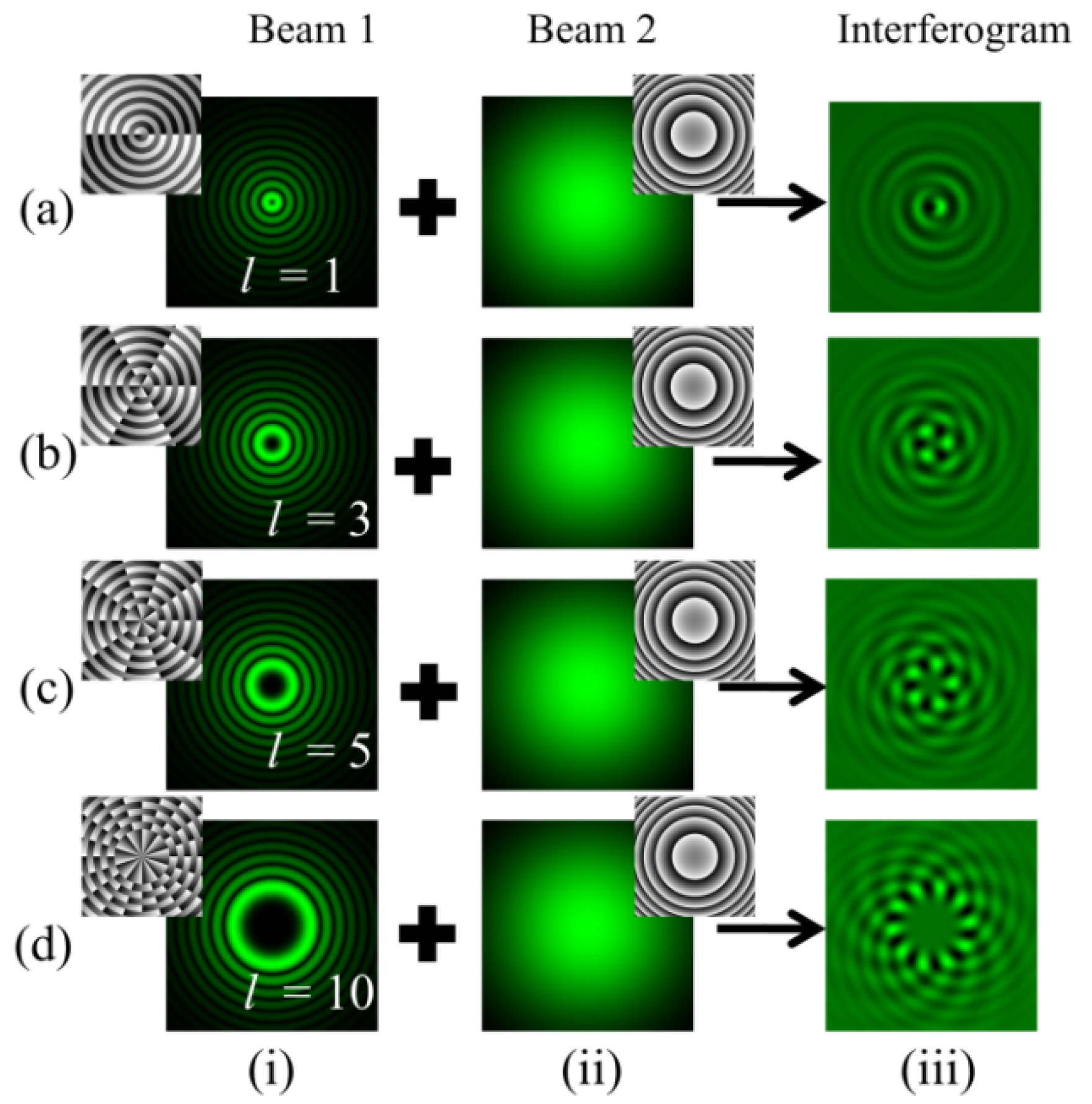
3.2. Interference of BG Beams with Spherical Beams

A.
In-line interference of the Bessel beam with a spherical beam
In-line interference of a BG beam with a spherical reference beam produces an interferogram consisting of spiral strips extending outward from the singular point, the number of which is related to its TC. The mathematical expression of a spherical beam is expressed as
E s = B 0 exp i k x 2 + y 2 2 w
where B0 denotes the intensity distribution and k = 2π/λ is the wavenumber of the field. w denotes the radius of curvature of the wavefront. Figure 6 depicts the interferogram obtained for different orders of BG beams. Column (i) represents the intensity distributions of BG beams of different order l = 1, 3, 5, and 10 as depicted in rows (a–d). Column (ii) describes the intensity distributions of spherical beams. Column (iii) represents the obtained intensity distribution of fringe patterns.

4. BG Beam Interference with Its Copy

Nevertheless, the availability of an independent reference beam for interference is not always guaranteed. This challenge has driven the creation of self-referenced interferometric techniques. In this method, the BG beam is interfered with with its own amplitude or wavefront split copy. As a result, self-referenced interferometric techniques offer more intuitive means for determining TC with simpler implementation.
In this study, we use the MZI framework for determining the TC of BG beams. The schematic of the modified MZI is shown in Figure 7. The desired BG beam of order +l whose phase distribution is to be determined, is directed into the interferometer. The beam is split into its amplitude copy along the orthogonal directions through a beam splitter (BS1). In the upper arm of the MZI, one of the split copies of the BG beam is passed through a right-angle prism (RAP). Hence, it is introduced with an extra path length or phase delay of δ = −0.1π and becomes completely internally reflected within the RAP. After passing through a RAP and reflecting from a mirror (M1), it is achieved without any modification in the wavefront. However, another split copy traversing in the lower arm of the MZI undergoes inversion in wavefront helicity. This is caused by three reflections from M2, BS2, and BS3. Both of the split amplitude copies are finally superposed using BS3 and captured by the camera. Employing the MZI configuration, we studied in-line as well as off-axis interference between the BG beam of +l and its conjugate of the −l order.

4.1. In-Line Interference of the Bessel Beam with Its Conjugate

The BG beam of order +l traversing in the upper arm of the MZI, which is introduced with a phase delay, and misalignment using mirror M1 are described as
E B G + l r ; ϕ , z = A l J l k r r exp i l ϕ exp r 2 w 0 2 × exp i δ × exp i 2 π λ y tan θ
where ϕ = tan 1 y x is the azimuth phase circulating around the optical axis of propagation of BG beams. δ is the additional phase delay introduced between the two amplitude-split copies of the BG beam. θ rrepresents the tilt introduced within one of the wavefront split copies of the BG beam. The wavefront split copy of the BG beam, which becomes conjugate of order −l after three reflections from M2, BS2, and BS3 is described as
E B G l r , ϕ , z = A l J l k r r exp i l ϕ exp r 2 w 0 2
The BG beam of order +l and its conjugate of order −l are interfered with using the MZI. The expression representing their superposition is expressed mathematically as
E r , ϕ , z = E B G + l r , ϕ , z × exp i δ × exp i 2 π λ y tan θ + E B G l r , ϕ , z
The resultant intensity of the two superposing BG beams is expressed as
I = E B G l + E B G + l exp i δ 2
In the case of in-line interference between the BG beam of order +l and its conjugate of order −l, the tilt introduced in one of the amplitude-split copies of the BG beam is set to θ = 0°, ensuring both beam cross-sections interfere at the camera plane. A phase delay of δ = −0.2π is introduced between two interfering beams. Figure 8 shows the interferogram obtained by in-line superposition of the BG beam of order +l with its conjugate of order −l. In this case, an interferogram consisting of petals is produced. It is observed that the petal fringes are uniformly and radially distributed. The intensity distribution gradually decreases as we move away from the center. The angular separation between the two adjacent fringes, denoted as α, is intrinsically linked to the TC through the relation α = π/l. This association implies that the magnitude of the TC, represented as |l|, is reciprocally related to the number of bright petals, denoted as n, with the expression |l| = n/2. Exploiting this relationship, the magnitude of the TC can be determined simply by counting the fringes. Figure 8 presents the simulation results for the intensity of fringe patterns obtained for TC values +1, +3, +5, +10, and +20. Row (a) presents the interference pattern obtained for the TC value as l = 1. Here, the total number of petals is 2, which gives the TC of the BG beam as 1. Similarly, in the case of the BG beam having l = 10 as shown in row (d), the number of petals achieved is 20, giving the TC value of10. Figure 9 shows the results for BG beams associated with the TC value as l = −1, −3, −5. Comparing these fringe patterns with the BG beam having positive TC values, it is observed that similar petal fringe patterns are produced for both + l and −l TC values, differing in the flip of petal structure. However, distinguishing the sign of the TC values for the petal-shaped fringe pattern is difficult. We observe that the size of the central dark region increases with the increase in the number of petals for higher-order TC values. The angle between the two neighboring fringes is determined by α = π/l, so for l = 30, α is 6°. Therefore, it gradually becomes challenging to determine TC for higher orders, like 100 and more.

4.2. Off-Axis Interference of the Bessel Beam with Its Conjugate

A simulation study has been carried out to produce off-axis interference, as described in Figure 10. The approach is to superpose a BG beam of order +l with its conjugate copy of order +l at a small tilt angle, ensuring their cross-sections overlap at the output plane. The small tilt angle is introduced in the beam wavefront traversing in the upper arm of the MZI using mirror M1. Incorporating a misalignment of 0.6° in the BG beam wavefront traversing in the upper arm of the MZI will result in the desired fork-shaped interference pattern. Mirror M1 can control both the tilt and lateral displacements to be introduced with the wavefront of the beam. The obtained fringe pattern bifurcates at the wavefront dislocation region. The fringe structure consists of a handle and tines coming out of it. The bright, discontinuous fringes encircling the singular region in the interference fringe pattern provide direct insight into the magnitude of the TC carried by the BG beam. The magnitude of the TC is determined by counting the number of tines using the relation |l| = (m +1)/2, where m represents the count of additional discontinuous bright fringes.
The intensity distributions of the desired interference patterns have been numerically evaluated and are shown in Figure 10. It describes fringe patterns for different orders of BG beams as l = +1, +3, +5, +10, +20, +30. The phase patterns are also depicted, corresponding to each order of superposing BG beams. Figure 11 depicts the fringe patterns obtained in cases of negative TC values such as l = −1, −3, −5. It is observed that for negative TC values, the fringe pattern lies at the position below the fringe defect. Conversely, in the case of positive TC values, this pattern completely reverses with the discontinuous fringes inverting and relocating at the position above the fringe defect. Therefore, these observations provide a means to differentiate the sign of the TC through the analysis of fringe patterns.

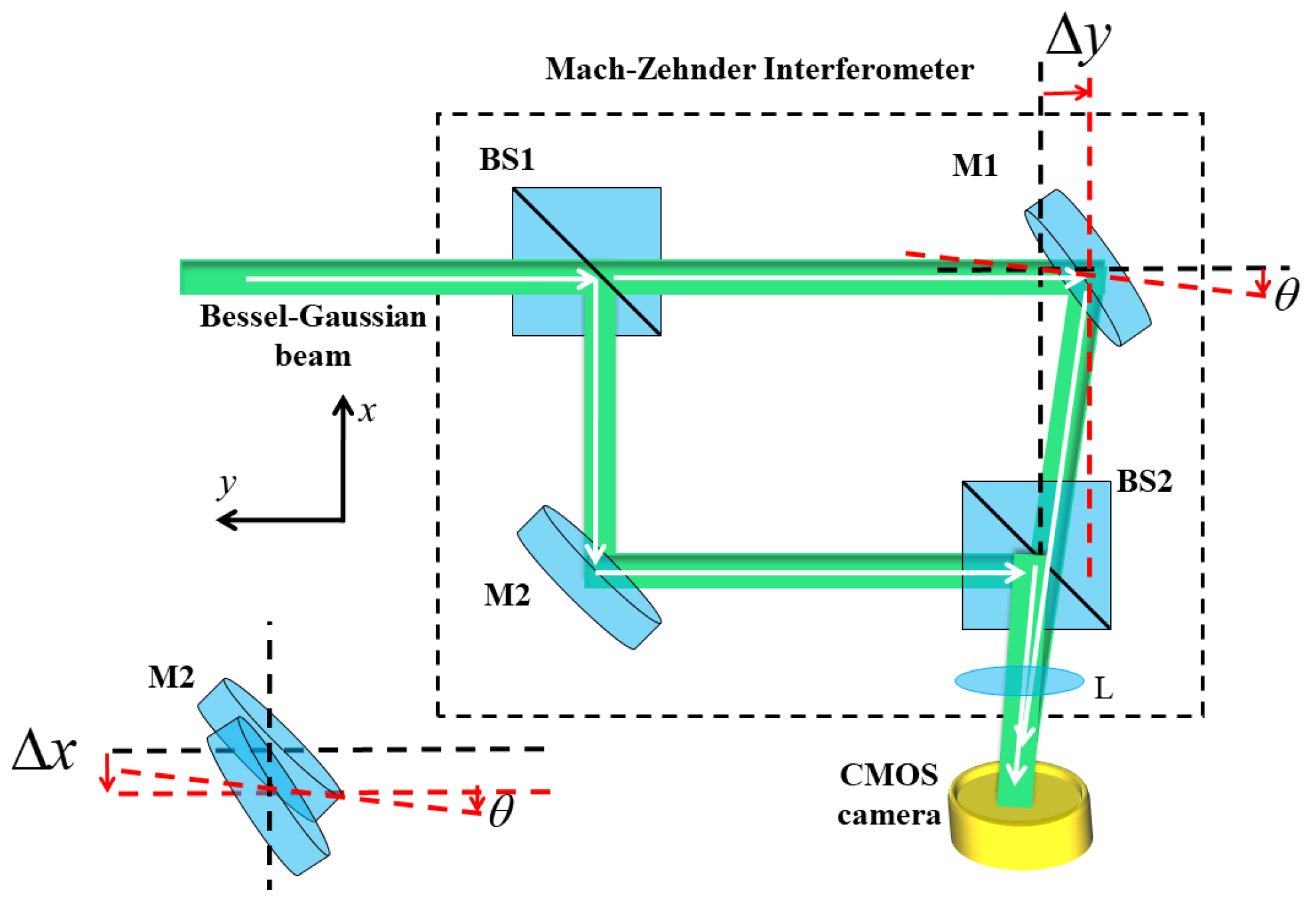
4.3. Self-Referencedinterference of BG Beams with TheirLaterally Displaced and Misaligned Amplitude-Split Copies

In this section, we discuss the interference between the BG beam and its own amplitude-split copy, which is laterally displaced and misaligned. This is known as the self-referenced interferometric approach, which is carried out using an MZI. The schematic diagram for producing self-referenced interference is shown in Figure 12. Here, the BG beams whose TC is to be determined enterthe MZI and are split into orthogonal directions using BS1. One of the copies, which is traversing into the upper arm of the MZI undergoes lateral displacement and misalignment through mirror M1, ensuring that both beams travel the same distance in both arms. Both the split copies are then interfered with using BS2 at the observation plane. In the set-up, mirrors M1 and M2 can control both tilt and lateral displacements to be introduced with the wavefront of the beam. Mirror M1 is rotated by an angle θ in the −x-direction and is displaced in the direction of tilt, producing adjacent two-forked fringes. Whereas in another case, mirror M2 is rotated by an angle θ in the −x-directionand is displaced in the −x-direction, producing a conjoined two-forked fringe pattern. Tilt causes displacement in the wavefront of the beam.
The electric field distribution of the amplitude-split copy of BG beam +l, which is laterally displaced along negative x and y directions and tilted in the x-direction, is described as
E x + Δ x 2 + y 2 , ϕ x + Δ x , y , z = E B G + l x , y ; ϕ x , y , z + E B G + l x + Δ x , y ; ϕ x + Δ x , y , z × exp i 2 π λ y tan θ E x 2 + y + Δ y 2 , ϕ x , y + Δ y , z = E B G + l x , y + Δ y ; ϕ x , y + Δ y , z × exp i 2 π λ y tan θ + E B G + l x , y ; ϕ x , y , z
The resultant intensity of the two superposing BG beams is expressed as
I = E B G + l x , y ; ϕ x , y , z + E B G + l x + Δ x , y ; ϕ x + Δ x , y , z × exp i 2 π λ y tan θ 2 I = E B G + l x , y + Δ y ; ϕ x , y + Δ y , z × exp i 2 π λ y tan θ + E B G + l x , y ; ϕ x , y , z 2
A.
Lateral displacement and tilt in the same direction
In this case, the BG beam of order +l interferes with its copy of order +l, which is laterally displaced in the −y direction and also tilted in the same direction. Mathematically, y = 0.17   m m , Δ x = 0 , and θ = −0.2° are substituted in Equation (13). In the set-up, mirror M1 is rotated by an angle θ and is displaced in the direction of the tilt. The resulting interferogram consists of two fork dislocations, as shown in Figure 13. The fringe pattern bifurcates at two adjacent locations of wavefront dislocations. The bright discontinuous fringes give the magnitude of the TC, which is determined by counting the number of tines using the relation |l| = m, where m represents the count of discontinuous bright fringes. Columns (i, ii) of rows (a–c) depict the intensity as well as phase profile distributions of the two interfering BG beams of different orders l = 1, 3, 5, respectively. The intensity-null centers of one of the interfering beams are displaced along the −y direction. The phase distributions are also seen laterally displaced and misaligned along the −y direction with respect to the other beam.
B.
Lateral displacement and tilt in the orthogonal direction
In this case, the BG beam of order +l interferes with its copy of order +l, which is tilted in the −y direction and laterally displaced in the orthogonal −x direction. Mathematically, Δ x = 0.17 mm , Δ y = 0 , and θ = −0.2° are substituted in Equation (13). Mirror M2 is rotated by an angle θ and is displaced in the −x-direction. The resulting interferogram consists of two conjoined forkeddislocations, as shown in Figure 14. The fringe pattern bifurcates at two adjacent locations of wavefront dislocations. The bright discontinuous fringes give the magnitude of the TC, which is determined by counting the number of tines using the relation |l| = m, where m represents the count of discontinuous bright fringes. Columns (i, ii) of rows (a–c) depict the intensity as well as phase profile distributions of the two interfering BG beams of different orders l = 1, 3, 5. The intensity null centers of both the interfering beams are displaced along the −x direction.

5. Verifying Propagation Propertiesand the TC of Phase-Truncated BG Beams

In this section, we examine the propagation propertiesand phase distribution within BG beams after they are obstructed by an aperture. The phases of BG beams are truncated using circular apertures of varying radii. The propagation of BG beams is then studied after encountering obstacles. Remarkably, the self-healing effect comes into play, allowing for TC determination after a long propagation distance. The detection of the TC intruncated BG beams reveals their self-healed intensity profile.
Here, we realize the self-healing effect through theoretically evaluated intensity distribution plots for BG beams of different orders. Figure 15 rows (a, b) represent the intensity distributions of BG beams obstructed by a circular aperture of radii r = 0.1, 0.13 mm at different propagation distances as d = 30, 50, 80, 100, 200, and 300 cm, respectively. Column (i) represents the intensity of BG beams of order l = 0 without obstacles while column (ii) represents the intensity of BG beams of order l = 0 obstructed by a circular aperture of radii r = 0.1, 0.13 mm, as depicted in rows (a, b), respectively. Columns (iii–x) of rows (b, d) represent the theoretical absolute value of intensity plots carried out when BG beams propagated at different propagation distances d = 30, 50, 80, 100, 200, and 300 cm, respectively. Similarly, Figure 16 rows (a, c) represent the intensity distributions of BG beams of order l = 1 and 5 obstructed by a circular aperture of radii r = 0.15, 0.3 mm at different propagation distances d = 30, 50, 80, 100, 200, 300, and 500 cm, respectively. Rows (a, b) of column (i) represent the intensity of BG beams of order l = 1 and 5 without obstacles, while column (ii) representsthe intensity of BG beams of order l = 1 and 5 obstructed by a circular aperture of radii r = 0.15, 0.3 mm. Columns (iii–x) and rows (b, d) represent the theoretical absolute values of the intensity plots carried out when BG beams of order l = 1 and 5 propagated at different propagation distances d = 30, 50, 80, 100, 200, 300, and 500 m, respectively. We realize from the intensity plots that the BG beams self-heal their intensity profiles at long propagation distances. Within the region of the truncated phase, it was completely dark, which gradually healedafter a certain propagation distance.
Our main aim in this paper is to determine the phase distribution within BG beams, which are truncated in phase upon encountering an obstacle while traversing. At this point, the phase-truncated BG beams are directed into the MZI. Here, both the amplitude-split copy of truncated BG beams arepropagated in the upper and lower arms of the MZI and then interfered with using BS2 at the imaging plane. Let zbethe distance between the source and the observation plane. The field distributions of both the BG beams traversing in the upper and lower arms of the MZI are calculated at the observation plane according to the Fresnel diffraction solution [53] using
E B G + l x , y = e i k z i λ z E B G + l x , y exp i k 2 z x x 2 + y y 2 d x d y
E B G l x , y = e i k z i λ z E B G l x , y exp i k 2 z x x 2 + y y 2 d x d y
Figure 15 and Figure 16 describe the path of one of the split copies of a truncated BG beam in one of the arms of the MZI at different distances, ensuring all other parameters remain the same.
Figure 17 represents the interference pattern of BG beams of different orders after they are obstructed by an aperture of varying radii. Using the MZI, in-line as well as off-axis interference patterns have been studied between a truncated BG beam of order +l and its conjugate amplitude-split copies, which are shown in Figure 15 and Figure 16. Rows (a, b) of Figure 17 represent the off-axis and in-lineinterference patterns obtained for obstructed BG beams. Columns (i, ii) of Figure 17 represent the interference pattern of a BG beam of order l = 0 when obstructed by circular aperture of radii r = 0.1, 0.13 mm, respectively. The in-line superposition gives a non-vortex center, which directly relates to the TC value as l = 0. Columns (iii, iv) of Figure 17 represent the interference pattern of BG beamsof order l = 1, 5when each is obstructed by a circular aperture of radii r = 0.15, 0.3 mm, respectively. The off-axis as well asin-line superposition through the MZI gives fork- and petal-shaped fringe patterns, respectively. In Figure 17, column (iii) of row (a), we determine the magnitude of the TC by counting the number of bright tines and then using the relation |l| = (m +1)/2, where m represents the count of additional discontinuous bright fringes. This gives the TC value of the BG beam as l = 1. In Figure 17, column (iv) of row (b) represents the petal fringe pattern. Here, we obtain the TC value using the relation |l| = n/2. With these observations, we successfully achieved the phase distribution within truncated-phase BG beams using the MZI.
This examination helps realize the self-healing behavior of BG beams, preserving their unique characteristics, despite encountering obstacles during propagation. Their self-healed intensity profile is verified with theoretical absolute values of intensity distribution plots and by determining the phase distribution within them.

6. Conclusions

In conclusion, this study presents different interferograms utilizing different MZI interferometric configurations to effectively determine the order of singularity within BG beams. Moreover, this study analyzes the efficient utilization of the MZI to determine the phase distribution within BG beams whose phases are truncated by different radii of circular apertures while propagating. Here, the propagation effects of phase-truncated beams were studied. This examination helps to explore how BG beams self-heal, preserving distinctive traits like the phase distribution in them, over extended distances despite truncation or obstacles.

Author Contributions

Investigation, M.B.; Writing—original draft, M.B.; Supervision, N.K.N. All authors have read and agreed to the published version of the manuscript.

Funding

Council of Scientific and Industrial Research, Govt. of India, under grant No. 03/1492/23/EMR-II.

Institutional Review Board Statement

Not applicable.

Informed Consent Statement

Not applicable.

Data Availability Statement

The data presented in this study are available on request from the corresponding author.

Acknowledgments

The authors acknowledge the funding from the Council of Scientific and Industrial Research, Govt. of India, under grant No. 03/1492/23/EMR-II.

Conflicts of Interest

The authors declare no conflict of interest.

References

  1. Bouchal, Z. Resistance of nondiffracting vortex beams to amplitude and phase perturbations. Opt. Commun. 2002, 210, 155–164. [Google Scholar] [CrossRef]
  2. Tao, S.H.; Yuan, X. Self-reconstruction property of fractional Bessel beams. J. Opt. Soc. Am. A 2004, 21, 1192–1197. [Google Scholar] [CrossRef]
  3. Fischer, P.; Little, H.; Smith, R.L.; Lopez-Mariscal, C.; Brown, C.T.A.; Sibbett, W.; Dholakia, K. Wavelength dependent propagation and reconstruction of white light Bessel beams. J. Opt. A 2006, 8, 477–482. [Google Scholar] [CrossRef]
  4. Chu, X. Analytical study on the self-healing property of Bessel beam. Eur. Phys. J. D 2012, 66, 259. [Google Scholar] [CrossRef]
  5. Bouchal, Z.; Wagner, J.; Chlup, M. Self-reconstruction of a distorted nondiffracting beam. Opt. Commun. 1998, 151, 207–211. [Google Scholar] [CrossRef]
  6. Yu, A.; Wu, G. Self-healing properties of optical pin beams. J. Opt. Soc. Am. A 2023, 40, 2078–2083. [Google Scholar] [CrossRef]
  7. Zhao, S.; Zhang, W.; Wang, L.; Li, W.; Gong, L.; Cheng, W.; Chen, H.; Gruska, J. Propagation and self-healing properties of Bessel-Gaussian beam carrying orbital angular momentum in an underwater environment. Sci. Rep. 2019, 9, 2025. [Google Scholar] [CrossRef]
  8. Yuan, Y.; Lei, T.; Li, Z.; Li, Y.; Gao, S.; Xie, Z.; Yuan, X. Beam wander relieved orbital angular momentum communication in turbulent atmospheric using Bessel beams. Sci. Rep. 2017, 7, 42276. [Google Scholar] [CrossRef]
  9. Otte, E.; Nape, I.; Guzman, C.R.; Valles, A.; Denz, C.; Forbes, A. Recovery of nonseparability in self-healing vector Bessel beams. Phy. Rev. A 2018, 98, 053818. [Google Scholar] [CrossRef]
  10. Aiello, A.; Agarwal, G.S.; Paur, M.; Stoklasa, B.; Hradil, Z.; Rehacek, J.; Hoz, P.D.L.; Leuchs, G.; Soto, L.L.S. Unraveling beam self-healing. Opt. Express 2017, 25, 19147–19157. [Google Scholar] [CrossRef]
  11. Khonina, S.N.; Kazanskiy, N.L.; Karpeev, S.V.; Butt, M.A. Bessel beam: Significance and applications-A progressive review. Micromachines 2020, 11, 997. [Google Scholar] [CrossRef] [PubMed]
  12. Duocastella, M.; Arnold, C.B. Bessel and annular beams for material processing. Laser Photon. Rev. 2012, 6, 607–621. [Google Scholar] [CrossRef]
  13. Stoian, R.; Bhuyan, M.K.; Zhang, G.; Cheng, G.; Meyer, R.; Courvoisier, F. Ultrafast Bessel beams: Advanced tools for laser material processing. Adv. Opt. Technol. 2018, 7, 165. [Google Scholar] [CrossRef]
  14. Li, S.; Wang, J. Adaptive free-space optical communications through turbulence using self-healing Bessel beams. Sci. Rep. 2017, 7, 43233. [Google Scholar] [CrossRef]
  15. Nape, A.; Otte, E.; Valles, A.; Guzman, C.R.; Cardano, F.; Denz, C.; Forbes, A. Self-healing high-dimensional quantum key distribution using hybrid spin-orbit Bessel states. Opt. Express 2018, 26, 26946–26960. [Google Scholar] [CrossRef]
  16. Lu, Z.; Guo, Z.; Fan, M.; Guo, M.; Li, C.; Yao, Y.; Zhang, H.; Lin, W.; Liu, H.; Liu, B. Tunable bessel beam shaping for robust atmospheric optical communication. J. Light. Technol. 2022, 40, 5097–5106. [Google Scholar] [CrossRef]
  17. Chavez, V.G.; Mcgloin, D.; Melville, H.; Sibbett, W.; Dholakia, K. Simultaneous micromanipulation in multiple planes using a self-reconstructing light beam. Nature 2002, 419, 145–147. [Google Scholar] [CrossRef]
  18. Planchon, T.A.; Gao, L.; Milkie, D.E.; Davidson, M.W.; Galbraith, J.A.; Betzig, E. Rapid three-dimensional isotropic imaging of living cells using Bessel beam plane illumination. Nat. Methods 2011, 8, 417–423. [Google Scholar] [CrossRef] [PubMed]
  19. Arlt, J.; Dholakia, K. Generation of high-order Bessel beams by use of an axicon. Opt. Commun. 2000, 177, 297–301. [Google Scholar] [CrossRef]
  20. Butt, M.A.; Savelyev, D. Bessel beams produced by axicon and spatial light modulator: A brief analysis. In Proceedings of the 2021 International Conference on Information Technology and Nanotechnology (ITNT), Samara, Russia, 20–24 September 2021. [Google Scholar]
  21. Vasara, A.; Turunen, J.; Friberg, A.T. Realizing of general nondiffracting beams with computer-generated hologram. J. Opt. Soc. Am. A 1989, 6, 1748–1754. [Google Scholar] [CrossRef] [PubMed]
  22. Zhai, Z.; Cheng, Z.; Lv, Q.; Wang, X. Tunable axicons generated by spatial light modulator with high-level phase computer-generated holograms. Appl. Sci. 2020, 10, 5127. [Google Scholar] [CrossRef]
  23. Tudor, R.; Bulzan, G.A.; Kusko, M.; Kusko, C.; Avramescu, V.; Vasilache, D.; Gavrila, R. Multilevel spiral axicon for high-order Bessel-Gauss beams generation. Nanomaterials 2023, 13, 579. [Google Scholar] [CrossRef] [PubMed]
  24. Sun, Q.; Zhou, K.; Fang, G.; Liu, Z.; Liu, S. Generation of spiraling high-order Bessel beams. Appl. Phys. B 2011, 104, 215–221. [Google Scholar] [CrossRef]
  25. Qi, M.Q.; Tang, W.X.; Cui, T.J. A broadband Bessel beam launcher using metamaterial lens. Sci. Rep. 2015, 5, 11732. [Google Scholar]
  26. Cox, A.J.; Dibble, D.C. Nondiffracting beam from a spatially filtered Fabry–Perot resonator. JOSA A 1992, 9, 282–286. [Google Scholar] [CrossRef]
  27. Horvath, Z.L.; Erdélyi, M.; Szabo, G.; Bor, Z.; Tittel, F.K.; Cavallaro, J.R. Generation of nearly nondiffracting Bessel beams with a Fabry-Perot interferometer. JOSA A 1997, 14, 3009–3013. [Google Scholar] [CrossRef]
  28. Reddy, V.; Bertoncini, A.; Liberale, C. 3D-printed fiber-based zeroth-and high-order Bessel beam generator. Optica 2022, 9, 645–651. [Google Scholar] [CrossRef]
  29. Rao, A.S. Origin, Experimental Realization, Illustrations, and Applications of Bessel beams: A Tutorial Review. arXiv 2024, arXiv:2401.04307. [Google Scholar]
  30. Baliyan, M.; Shikder, A.; Nishchal, N.K. Generation of structured light beams by dual phase modulation with a single spatial light modulator. Phys. Scr. 2023, 98, 105528. [Google Scholar] [CrossRef]
  31. Baliyan, M.; Nishchal, N.K. Generating scalar and vector modes of Bessel beams utilizing holographic axicon phase with spatial light modulator. J. Opt. 2023, 25, 095702. [Google Scholar] [CrossRef]
  32. Durnin, J. Exact solutions for nondiffracting beams. I. Scalar Theory J. Opt. Soc. Am. A 1987, 4, 651–654. [Google Scholar] [CrossRef]
  33. Durnin, J. Diffraction-free beams. Phys. Rev. Lett. 1987, 58, 1499–1501. [Google Scholar] [CrossRef]
  34. Berry, M.V. Optical vortices evolving from helicoidal integer and fractional phase steps. J. Opt. A Pure Appl. Opt. 2004, 6, 259–268. [Google Scholar] [CrossRef]
  35. Kotlyar, V.V.; Kovalev, A.A.; Volyar, A.V. Topological charge of a linear combination of optical vortices: Topological competition. Opt. Express 2020, 28, 8266–8281. [Google Scholar] [CrossRef]
  36. Shen, Y.; Wang, X.; Xie, Z.; Min, C.; Fu, X.; Liu, Q.; Gong, M.; Yuan, X. Optical vortices 30 years on: OAM manipulation from topological charge to multiple singularities. Light Sci. Appl. 2019, 8, 90. [Google Scholar] [CrossRef]
  37. Ferreira, Q.S.; Jesus-Silva, A.J.; Fonseca, E.J.; Hickmann, J.M. Fraunhofer diffraction of light with orbital angular momentum by a slit. Opt. Lett. 2011, 36, 3106–3108. [Google Scholar] [CrossRef]
  38. Sztul, H.I.; Alfano, R.R. Double-slit interference with Laguerre-Gaussian beams. Opt. Lett. 2006, 31, 999–1001. [Google Scholar] [CrossRef] [PubMed]
  39. Hickmann, M.; Fonseca, E.J.S.; Soares, W.C.; Chávez-Cerda, S. Unveiling a truncated optical lattice associated with a triangular aperture using light’s orbital angular momentum. Phys. Rev. Lett. 2010, 105, 053904. [Google Scholar] [CrossRef]
  40. Alperin, S.N.; Niederriter, R.D.; Gopinath, J.T.; Siemens, M.E. Quantitative measurement of the orbital angular momentum of light with a single, stationary lens. Opt. Lett. 2016, 41, 5019–5022. [Google Scholar] [CrossRef]
  41. Vaity, P.; Banerji, J.; Singh, R.P. Measuring the topological charge of an optical vortex by using a tilted convex lens. Phys. Lett. A 2013, 377, 1154–1156. [Google Scholar] [CrossRef]
  42. Bazhenov, V.Y.; Vasnetsov, M.V.; Soskin, M.S. Laser beam with screw dislocations in their wavefronts. Pis’ma Zh. Eksp. Teor. Fiz. 1990, 52, 1037–1039, Erratum in JETP Lett. 1990, 52, 429–431. [Google Scholar]
  43. Pan, S.; Pei, C.; Liu, S.; Wei, J.; Wu, D.; Liu, Z.; Yin, Y.; Xia, Y.; Yin, J. Measuring orbital angular momentums of light based on petal interference patterns. OSA Contin. 2018, 1, 451–461. [Google Scholar] [CrossRef]
  44. Senthilkumaran, P.; Masajada, J.; Sato, S. Interferometry with vortices. Int. J. Opt. 2011, 2012, 517591. [Google Scholar] [CrossRef]
  45. Lan, B.; Liu, C.; Rui, D.; Chen, M.; Shen, F.; Xian, H. The topological charge measurement of the vortex beam based on dislocation self-reference interferometry. Phys. Scr. 2019, 94, 055502. [Google Scholar] [CrossRef]
  46. Fedorov; Gavril’eva, K.; Gorelaya, A.; Sevryugin, A.; Tursunov, I.; Venediktov, D.; Venediktov, V. Reference beam lacking measurement of topological charge of incoming vortex beam. Proc. SPIE 2019, 11030, 1103002. [Google Scholar]
  47. Ghai, P.; Vyas, S.; Senthilkumaran, P.; Sirohi, R.S. Detection of phase singularity using a lateral shear interferometer. Opt. Lasers Eng. 2008, 46, 419–423. [Google Scholar] [CrossRef]
  48. Ghai, P.; Senthilkumaran, P.; Sirohi, R.S. Shearograms of an optical phase singularity. Opt. Commun. 2008, 281, 1315–1322. [Google Scholar] [CrossRef]
  49. Kumar, P.; Nishchal, N.K. Self-referenced interference of laterally displaced vortex beams for topological charge determination. Opt. Commun. 2020, 459, 125000. [Google Scholar] [CrossRef]
  50. Cui, S.; Xu, B.; Luo, S.; Xu, H.; Cai, Z.; Luo, Z.; Pu, J.; Chávez-Cerda, S. Determining topological charge based on an improved Fizeau interferometer. Opt. Express 2019, 27, 12774–12779. [Google Scholar] [CrossRef]
  51. Li, X.; Tai, Y.; Zhang, L.; Nie, Z.; Chen, Q. High-order topological charges measurement of LG vortex beams with a modified Mach-Zehnder interferometer. Optik 2015, 126, 4378–4381. [Google Scholar]
  52. Guo, J.; Guo, B.; Fan, R.; Zhang, W.; Wang, Y.; Zhang, L.; Zhang, P. Measuring topological charges of Laguerre–Gaussian vortex beams using two improved Mach-Zehnder interferometers. Opt. Eng. 2016, 55, 035104. [Google Scholar] [CrossRef]
  53. Kumar, P.; Nishchal, N.K. Modified Mach–Zehnder interferometer for determining the high-order topological charge of Laguerre-Gaussian vortex beams. J. Opt. Soc. Am. A 2020, 36, 1447–1455. [Google Scholar] [CrossRef] [PubMed]
  54. Volyar, A.; Abramochkin, E.; Egorov, Y.; Bretsko, M.; Akimova, Y. Fine structure of perturbed Laguerre-Gaussian beams: Hermite-Gaussian mode spectra and topological charge. Appl. Opt. 2020, 59, 7680–7687. [Google Scholar] [CrossRef] [PubMed]
Figure 1. Schematic diagram of the experimental set-up for BG beam generation. Dotted red represent modulation within component of light field.
Photonics 11 00263 g001
Figure 2. Schematic representing in-line interference of BG beams with a reference beam. Green dotted represent reference beam after reflection from mirror while red represent interfered reference and BG beam.
Photonics 11 00263 g002
Figure 3. Simulation results of an in-line interferogram obtained after interference of BG beams with a Gaussian beam. Column (i): intensity distributions of BG beams of different orders l = 1, 3, 5, and 10 as depicted in rows (a–d). Column (ii): intensity distributions of Gaussian beams. Column (iii): intensity distributions of fringe patterns.
Photonics 11 00263 g003
Figure 4. Schematic diagram representing off-axis interference of BG beams with a Gaussian beam. Green dotted represent misaligned reference beam after reflection from mirror while red represent interfered reference and BG beam.
Photonics 11 00263 g004
Figure 5. Simulation results of an off-axis interferogram obtained after interference of BG beams with a Gaussian beam. Column (i): intensity distributions of BG beams of different orders l = 1, 3, 5, and 10 as depicted in rows (a–d). Column (ii): intensity distributions of Gaussian beams. Column (iii): intensity distributions of fringe patterns.
Photonics 11 00263 g005
Figure 6. Simulation results of an in-line interferogram obtained after interference of BG beams with a spherical beam. Column (i): intensity distributions of BG beams of different orders l = 1, 3, 5, and 10 as depicted in rows (a–d). Column (ii): intensity distributions of spherical beams. Column (iii): intensity distributions of fringe patterns.
Photonics 11 00263 g006
Figure 7. Schematic diagram of the modified MZI. BS1, BS2: beam splitter; M1, M2: mirror; RAP: right angle prism; CMOS camera: complementary metal-oxide semiconductor camera. Dotted red represent tilt introduced in the mirror.
Photonics 11 00263 g007
Figure 8. Simulation results of an inline interferogram obtained after interference of BG beams with their conjugate copies. Columns (i, ii) of rows (a–f): intensity distributions of BG beams of different orders l = 1, 3, 5, 10, and 20 and their conjugate copies. Column (iii): intensity distributions of the desired fringe patterns.
Photonics 11 00263 g008
Figure 9. Simulation results of in-line interference obtained after interference of BG beams with their conjugate copies. Columns (i, ii) of rows (a–c): intensity distributions of BG beams of different orders l = −1, −3, −5 and their conjugate copies. Column (iii): intensity distributions of the desired fringe patterns.
Photonics 11 00263 g009
Figure 10. Simulation results of the interference of BG beams with theirtilted conjugate copies. Columns (i, ii) of rows (a–f): intensity distributions of BG beams of different orders l = 1, 3, 5, 10, 20, 30 and their tilted conjugate copies. Column (iii): intensity distributions of the desired fringe patterns.
Photonics 11 00263 g010
Figure 11. Simulation results of the interference of BG beams with their tilted conjugate copies. Columns (i, ii) of rows (a–c): intensity distributions of BG beams of different orders l = −1, −3, −5 and and their tilted conjugate copies. Column (iii): intensity distributions of the desired fringe patterns.
Photonics 11 00263 g011
Figure 12. Schematic diagram of the modified MZI. Red dotted represent tilt and lateral displacement introduced in mirror M1 and M2.
Photonics 11 00263 g012
Figure 13. Simulation results of the interference of BG beams with their laterally displaced copies in the −y direction and tilted in the same direction. Rows (a–c):intensity distributions of BG beams of different orders l = 1, 3, 5. Columns (i, ii): intensity distributions of BG beams of different orders and their laterally displaced and tilted copies. Column (iii): intensity distributions of the desired fringe patterns.
Photonics 11 00263 g013
Figure 14. Simulation results of the interference of BG beams with their laterally displaced copies in the−y direction and tilted in the orthogonal –x direction. Rows (a–c):intensity distributions of BG beams of different orders l = 1, 3, 5. Columns (i, ii): intensity distributions of BG beams of different orders and their laterally displaced and tilted copies. Column (iii): intensity distributions of the desired fringe patterns.
Photonics 11 00263 g014
Figure 15. Simulation results of the intensity distribution of truncated-phase BG beams of order l = 0 at different propagation distances. Rows (a, c): intensity distributions of BG beams obstructed by a circular aperture of radii r = 0.1, 0.15 mm at different propagation distances d = 30, 50, 80, 100, 200, and 300 cm. Column (i): intensity of BG beams of order l = 0 without obstacles. Column (ii): intensity of BG beams of order l = 0 obstructed by a circular aperture of radii r = 0.1, 0.13 mm. rows (b, d): theoretical absolute values of intensity plots carried out when the BG beamspropagated at different propagation distances d = 30, 50, 80, 100, 200, and 300 cm as depicted in column (iii–viii). Green represents the intensity profile for the truncated BG beam and the red pattern represents the intensity profile of the theoretical absolute value of the BG beam.
Photonics 11 00263 g015
Figure 16. Simulation results of the intensity distribution of truncated-phase BG beams of order l = 1 and 5 at different propagation distances, respectively. Rows (a, c): intensity distributions of BG beams of order l = 1 and 5 obstructed by a circular aperture of radii r = 0.15, 0.3 mm at different propagation distances d = 30, 50, 80, 100, 200, 300, and 500 cm. Rows (a, c) of column (i): intensity of BG beams of order l = 1 and 5 without obstacles, Row (b) of column (i): theoretical absolute values of intensity of BG beams of order l = 1 and 5 without obstacles. Rows (a, c) of Column (ii): intensity of BG beams of order l = 1 and 5 obstructed by a circular aperture of radii r = 0.15, 0.3 mm. Rows (b) of column (i): theoretical absolute values of intensity of BG beams of order l = 1 and 5 without obstacles. Rows (b, d): theoretical absolute values of intensity plots carried out when BG beams of order l = 1 and 5 propagated at different propagation distances d = 30, 50, 80, 100, 200, 300, and 500 cm as depicted in columns (iii–viii).
Photonics 11 00263 g016
Figure 17. Interference patterns ofBG beams of different orders, after being obstructed by an aperture of varying radii. Rows (a, b): off-axis and in-lineinterference of obstructed BG beams as shown in Figure 15 and Figure 16 with their conjugate copies. Columns (i, ii): interference patterns of BG beamsof order l = 0 when obstructed by a circular aperture of radii r = 0.1, 0.15 mm. Column (iii, iv): interference patterns of BG beams of order l = 1, 5 when obstructed by a circular aperture of radii r = 0.15, 0.3 mm, respectively.
Photonics 11 00263 g017
Disclaimer/Publisher’s Note: The statements, opinions and data contained in all publications are solely those of the individual author(s) and contributor(s) and not of MDPI and/or the editor(s). MDPI and/or the editor(s) disclaim responsibility for any injury to people or property resulting from any ideas, methods, instructions or products referred to in the content.

