Communication

Optical Chaos in Saturated Nonlinear Media

College of Physical Science and Technology, Ningbo University, Ningbo 315211, China
*
Author to whom correspondence should be addressed.
Photonics 2023, 10(5), 600; https://doi.org/10.3390/photonics10050600
Submission received: 19 April 2023 / Revised: 15 May 2023 / Accepted: 19 May 2023 / Published: 22 May 2023

Abstract

:
In the study of the evolution of Gaussian beam in saturated nonlinear media, it is found that the probability of optical rogue waves changes with the change of nonlinearity. The light intensity distribution on the exit surface of nonlinear medium can be characterized by scintillation index, and the change of rogue wave corresponds to the evolution of scintillation index. The rogue wave probability shows a complex trend with the evolution of nonlinearity. The Lyapunov exponent and power spectrum method are used to determine that the probability of rogue wave is chaotic with nonlinear evolution.

1. Introduction

Chaos has always been a research hotspot. Chaos exists in all nonlinear systems, including optics [1,2,3], atmospheric science [4], finance [5], and celestial systems [6]. In the optical nonlinear system, the early studies of optical chaos are mainly related to the unstable output of the laser. In recent studies, it was found that chaos can be observed through the collision of multiple objects. By means of theoretical and experimental studies on the propogation of wave function in a medium [7,8,9,10,11], it has been discovered that a unique optical phenomenon, known as optical soliton [12], is produced when there is a balance between the diffraction and self-focusing of a Gaussian beam. According to numerical study, the solitons of the GrossPitaevskii equation or the Lorenz–Haken equation exhibit chaos after a three-soliton collision [13]. In a recent study, Xin experimentally observed optical chaos after collisions of three solitons in a saturated nonlinear medium [14]. It has been proved numerically and experimentally that the collision of three or more solitons will produce optical chaos [13]. Another soliton collision discovered that multiple soliton which possess a specific level of energy and quantity collisions are often accompanied by the generation of Rogue waves (RWs) [15,16].
In a recent study, Avigliano found that in photorefractiveally saturated nonlinear media under appropriate nonlinear conditions, the nonlinear evolution of a tightly focused Gaussian beam (Gb) exhibits a RW probability distribution, and this probability increases with the increase of the external electric field. This study shows that as the nonlinearity increases, the tightly focused Gb with perturbation splits into filaments, which collide with each other [17]. In the same year, Chen found that under appropriate nonlinear conditions in saturated nonlinear media, the nonlinear evolution of a wide Gb also exhibits the distribution of RW probability [18]. It is certain that the collision of the filaments generated after the splitting of the Gb can also produce RWs. Since the probability of RWs generated by filament collision is irregular with the evolution of nonlinearity, this has attracted our attention [15].
The modulation of nonlinear propagation of Gb in saturated nonlinear media is related to the applied voltage and beam intensity. In this work, we set a fixed beam intensity and change the applied voltage to change the nonlinearity.
In this work, we investigated the nonlinear evolution of RWs induced by a Gb with perturbation in a saturated nonlinear medium. We used the Lyapunov exponent [19,20,21] and power spectrum method [22,23,24] to study the existence of optical chaos through experiments and numerical simulations.

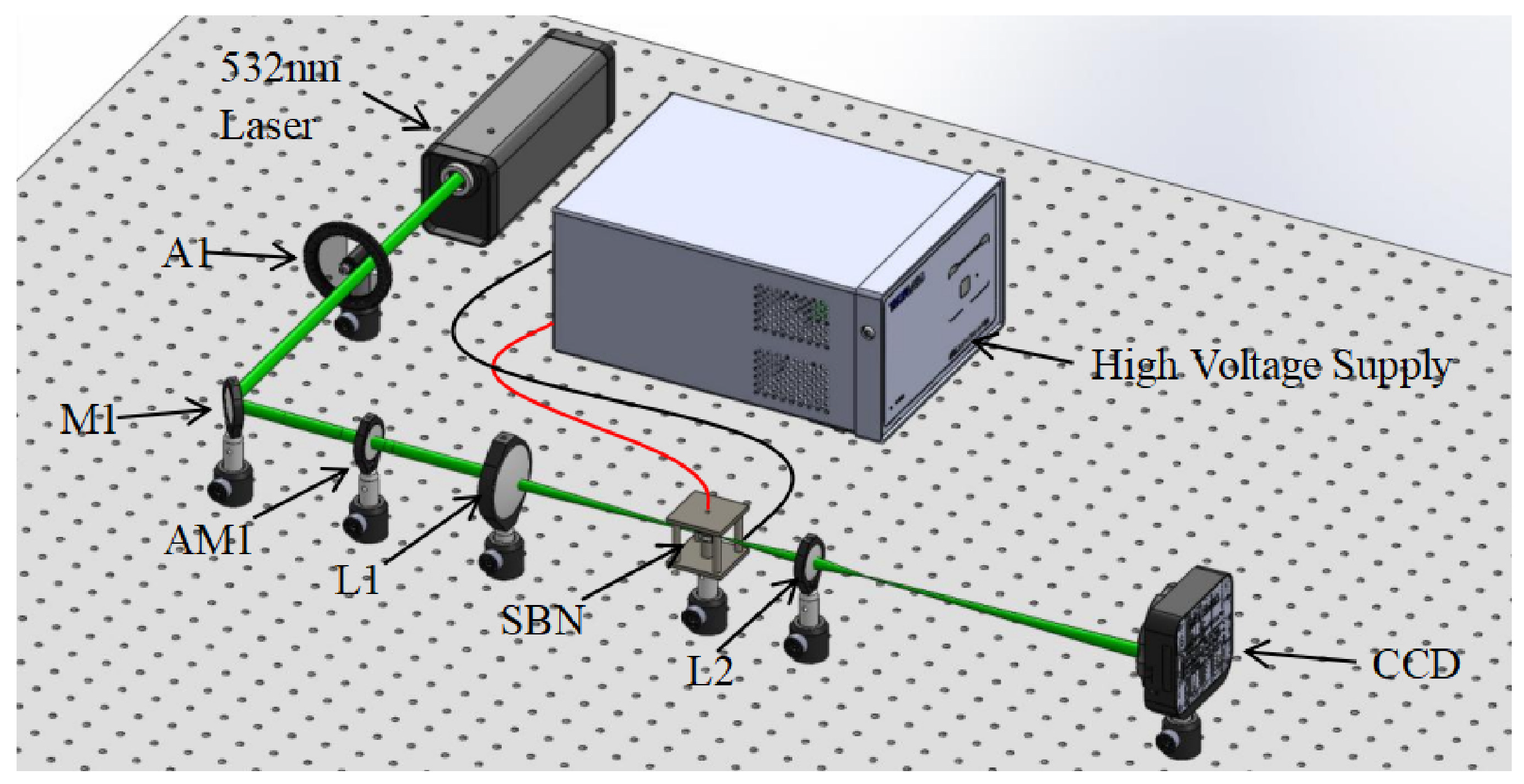
2. Experimental Setup

As shown in Figure 1, we used an SBN crystal with a cross-sectional area of 5 × 5 mm 2 and a length of 10 mm (propagation coordinate z). The saturation nonlinearity is adjusted by adjusting the applied voltage along the optical axis of the crystal. The incident light is a 532 nm wavelength laser with extraordinary polarization in the direction of the applied voltage. The beam width at half maximum is about 30 µm, and the input power is about 120 µW. A CCD camera is used to record the light intensity distribution profile at the input and output of the crystal.
The applied voltage was varied to observe and collect the intensity distribution after the nonlinear modulation was stabilized. The voltage was increased from 0 V to 900 V with a step size of 15 V. In order to perform RW statistics, the experiment was repeated 100 times under each voltage. When the applied voltage is 0 V, the spot size on the output surface of the saturated nonlinear crystal is 42 µm, which is larger than the input profile due to linear diffraction. The input light propagates along the z-axis, and it has a non-uniform Gb with a large amount of perturbation, which is about 1 % of the light intensity. The perturbation in the Gb is provided by an intensity mask AM1. These perturbations are important for splitting in the presence of nonlinearity.
Figure 2 shows the output beam profiles at various applied voltages. It can be seen that as nonlinearity increases, the perturbation in the incident light is gradually amplified in the propagation process, and the intensity distribution of the rear surface of the crystal shows a complex trend.
Statistical analysis of RWs was conducted on the experimental data. Statistics follow the following principles: to determine the probability of RWs, the event with the anomaly index A I = I / I e > 2 is regarded as RW. I is the intensity of each wave, and I e is defined as the average value of the highest intensity tertile of the corresponding probability density function (PDF) distribution.
As shown in Figure 3, the long tail distribution can be clearly observed by counting 100 sets of data at 510 V in the experiment.
The rogue wave probability under applied voltage is represented by P. We conduct rogue wave statistical analysis on the exit surface at different voltages using a total of 100 sets of experimental data [see Figure 4].
We used scintillation index to describe the intensity distribution [25]. The scintillation index ( S z ), which describes the average intensity gap of each filament is given as: S z = ( | I 2 | | I | 2 ) / | I | 2 , where | I 2 | is the average of the square of light intensity of each filament on the exit plane and | I | 2 is the square of the average light intensity of each filament. At the same voltage, 100 sets of experimental data were collected repeatedly, and the scintillation index was calculated as shown in Figure 5.
We averaged 100 groups of scintillation indexes. The results are shown in Figure 6.
When the scintillation index is compared to the RWs probability, it is clear that the two have the same evolution trend. By calculating the scintillation index and the probability of RWs, it can be analyzed that the scintillation index will increase when there is a strong spot. Similarly, the RW is a strong spot. The evolution of RWs probability with nonlinearity can be studied by studying the scintillation index.
We changed the incident light intensity to 99.5 % of the previous level using the A1 device, then collected the light intensity distribution on the rear surface by repeating the previous experimental steps, and calculated the scintillation index. The scintillation index as a function of applied voltage obtained from the two experiments is shown in Figure 7.
It can be seen, as the light intensity changed by 0.5%, the evolution of the scintillation index is very intense and unpredictable in the later stage of nonlinear change, which is chaos.
Chaos is defined as a type of quasi-random motion with a specific location. The evolution process of a chaotic system is very sensitive to the initial conditions. We calculated the Lyapunov exponent ( L E ) to determine whether the evolution is chaotic [21]. L E can be calculated as [26]:
L E = 1 N l o g Δ ( x n ) Δ ( x 0 ) = 1 N l o g d f n ( x 0 ) d x
where N is the length of the Scintillation index series, x n is the scintillation index, x 0 is the scintillation index of 0 V. L E can be divided into three types: when L E < 0 , the system converges to a fixed value; when L E = 0 , the system is in a stable state; when L E > 0 , the system diverges. The experimental data were reconstructed in phase space, and the time delay [27] and embedding dimension [28] were obtained by autocorrelation and false nearest neighbor methods, respectively. The calculation results are shown in Figure 8a,b.
The calculated time delay is represented by T, T = 3 , and the calculated embedding dimension is represented by m, m = 4 .
We calculated the largest Lyapunov exponent and obtain the result is 0.19. The results are shown in Figure 9. The result of the largest Lyapunov index is greater than 0. Therefore, the RWs probability is chaotic with the evolution of the applied voltage.
For the chaotic evolution of the light intensity distribution of the SBN crystal exit surface with the increase of voltage, we verify our results from the perspective of the power spectrum. The power spectrum is the corresponding spatial spectrum in the process of system evolution. The power spectrum of periodic motion is discrete, with only a few peaks at different frequencies. White noise is due to the completely random motion, and its power spectrum has no continuous broad peak. Chaos is a local quasi-random system with the characteristics of periodic motion and complete random motion. Its power spectrum should have broad peaks and continuous low-intensity sub-peaks [22]. The scintillation index image of Figure 6 is converted into the power spectrum. The calculation method is as follows:
X ( ω ) = n = 0 N 1 x ( n ) e i ω n
S ( ω ) = 1 N | X ( ω ) | 2
where x ( n ) is the scintillation index series, N is the length of the Scintillation index series, and S ( w ) is the power spectrum. In this paper, we use the nonlinear power spectrum.
Figure 10 shows the experimentally measured power spectrum of the scintillation index. A high-power main peak and several low-power secondary peaks can be seen. Therefore, it can be concluded that in a saturated nonlinear medium, the evolution of the RWs generated by a Gb under appropriate nonlinearity is chaotic.

3. Numerical Simulation

To verify the experimental findings, we numerically simulate the chaotic phenomena on SBN crystal and compare them with the experimental results. The distributed beam propagation method (BPM) is used for numerical simulation. The propagation of Gb in SBN crystal satisfies the nonlinear Schrodinger equation [29]:
i ( z ) ψ ( x , y , z ) + 1 2 k 0 2 ψ ( x , y , z ) = Δ n k 0 n e ψ ( x , y , z )
where 2 is the Laplacian operator, z is the propagation distance, ψ ( x , y , z ) is the slowly varying light wave envelope, k 0 = 2 π / λ is the wave vector, where λ is the wavelength of light, n e is the refractive index of the extraordinary polarized beam in the SBN crystal. The change in refractive index Δ n caused by the beam in SBN crystal can be given as:
Δ n = 1 2 n e 3 γ 33 E
where γ 33 is the electro-optic coefficient. E can be expressed as:
E = E 0 I d I + I d K B T e 1 I + I d I x
where I is the intensity of light irradiation, I d is the intensity of dark irradiation, E 0 is the external electric field, K B T is the product of Boltzmann constant and absolute temperature, and e is the electron charge.
The full width at half maximum of the incident Gb was set equal to 30 µm, respectively. By adding a noise seed to the incident light to simulate the perturbation in the incident light, the noise intensity is set to 2 % the amplitude of the incident light at the corresponding position. The lateral width of the crystal is 5 mm and the propagation length is 10 mm, with a refractive index n e of 2.33 and an electro-optic coefficient of 280 pm/V. The rule to change the applied voltage for adjusting saturation nonlinearity is as follows: increase the voltage from 0 V to 900 V with a step of 15 V.
Before the RWs statistics, taking the RWs statistics under 800 V voltage as an example. At an applied voltage of 800 V, we repeated the simulation for 100 times, and performed probability statistics on all the spots obtained. We found that there was an obvious long-tail distribution as shown in Figure 11.
At each voltage, we repeat the numerical simulation 100 times and count the Rw probability. The results are shown in Figure 12.
After counting the probability of RWs, the scintillation index is calculated for the exit surface under different voltages. Under different voltages, the statistical scintillation index of the light intensity distribution of 100 groups of exit surfaces is shown in Figure 13. We averaged 100 groups of scintillation indexes, and the results are shown in Figure 14. As shown in Figure 12 and Figure 14, the evolution trend of RWs probability and scintillation index is almost identical.
To check if the evolution of the scintillation index is sensitive to the initial condition, we reduced the incident light intensity by 0.5 % , and then repeated the above-described numerical simulation process. The results are shown in Figure 15.
Similarly, phase space reconstruction is performed on the simulated data. As shown in Figure 16, the time delay and embedding dimension are calculated by autocorrelation method and false nearest neighbor method. We calculate T = 2 , m = 4 .
The Lyapunov exponent was calculated by phase space reconstruction of the simulated data. As shown in Figure 17, the calculated maximum Lyapunov exponent is 0.21. The maximum Lyapunov exponent is positive, so the evolution of the RWs probability with nonlinearity is chaotic.
We also used the power spectrum method to verify the above results. The obtained results are shown in Figure 18. The power spectrum had the characteristics of wide peak and continuous sub-peak, which accorded with the power spectrum characteristics of chaos.
The simulation shows that as the voltage increases, RWs probability becomes chaotic.

4. Conclusions

Through statistical experiments and numerical simulations, Gaussian beams exhibit filamentation caused by modulation instability in saturated nonlinear crystals. The collision of spots after splitting is the main reason for the generation of RWs. In previous studies, the evolution of RWs probability with nonlinearity was not studied. The light intensity distribution of the exit surface is characterized by the scintillation index, and it is found that the scintillation index and the RWs probability are consistent with the trend of nonlinear evolution. It is proved by the Lyapunov exponent greater than 0 and the power spectrum with wide peak and continuous sub-peak characteristics that with the increase of nonlinearity, the probability of obtaining RWs is chaotic. In the following work, we will study the time evolution of Gb in SBN crystals under giant nonlinearity and the relationship between optical RWs and optical chaos.

Author Contributions

Methodology, F.L. and C.L.; software, F.L., J.S., M.L. and Z.C.; validation, F.L.; writing original draft: F.L.; writing—review & editing, F.L.; project administration, C.L.; funding acquisition, C.L. All authors have read and agreed to the published version of the manuscript.

Funding

This research was funded by National Natural Science Foundation of China (12074207).

Institutional Review Board Statement

Not applicable.

Informed Consent Statement

Not applicable.

Data Availability Statement

Data underlying the results presented in this paper are not publicly available at this time but may be obtained from the authors upon reasonable request.

Acknowledgments

Thank Hu Yi for his helpful discussion.

Conflicts of Interest

The authors declare no conflict of interest.

References

  1. Haken, H. Analogy between higher instabilities in fluids and lasers. Phys. Lett. A 1975, 53, 77–78. [Google Scholar] [CrossRef]
  2. Gibbs, H.M.; Hopf, F.A.; Kaplan, D.L.; Shoemaker, R.L. Observation of chaos in optical bistability. Phys. Rev. Lett. 1981, 46, 474. [Google Scholar] [CrossRef]
  3. Weiss, C.O.; Klische, W.; Ering, P.S.; Cooper, M. Instabilities and chaos of a single mode NH3 ring laser. Opt. Commun. 1985, 52, 405–408. [Google Scholar] [CrossRef]
  4. Lorenz, E.N. Deterministic nonperiodic flow. J. Atmos. Sci. 1963, 20, 130–141. [Google Scholar] [CrossRef]
  5. Wang, Z.; Huang, X.; Shi, G. Analysis of nonlinear dynamics and chaos in a fractional order financial system with time delay. Comput. Math. Appl. 2011, 62, 1531–1539. [Google Scholar] [CrossRef]
  6. Crawford, J.D. Introduction to bifurcation theory. Rev. Mod. Phys. 1991, 63, 991. [Google Scholar] [CrossRef]
  7. Huang, Z.; Zhu, W.; Feng, Y.; Deng, D. Spatiotemporal self-accelerating Airy–Hermite–Gaussian and Airy–helical–Hermite–Gaussian wave packets in strongly nonlocal nonlinear media. Opt. Commun. 2019, 441, 195–207. [Google Scholar] [CrossRef]
  8. Rodrigues Gonçalves, M.; Rozenman, G.G.; Zimmermann, M.; Efremov, M.A.; Case, W.B.; Arie, A.; Shemer, L.; Schleich, W.P. Bright and dark diffractive focusing. Appl. Phys. B 2022, 128, 51. [Google Scholar] [CrossRef]
  9. Rozenman, G.G.; Schleich, W.P.; Shemer, L.; Arie, A. Periodic wave trains in nonlinear media: Talbot revivals, Akhmediev breathers, and asymmetry breaking. Phys. Rev. Lett. 2022, 128, 214101. [Google Scholar] [CrossRef]
  10. Rozenman, G.G.; Shemer, L.; Arie, A. Observation of accelerating solitary wavepackets. Phys. Rev. E 2020, 101, 050201. [Google Scholar] [CrossRef]
  11. Chen, Y.; Hosseini, B.; Owhadi, H.; Stuart, A.M. Solving and learning nonlinear PDEs with Gaussian processes. J. Comput. Phys. 2021, 447, 110668. [Google Scholar] [CrossRef]
  12. Gupta, N. Multi Gaussian Breather Solitons in Diffraction Managed Nonlinear Optical Media. Nonlinear Opt. Quantum Opt. Concepts Mod. Opt. 2022, 55, 309–330. [Google Scholar]
  13. Dalfovo, F.; Giorgini, S.; Pitaevskii, L.P.; Stringari, S. Theory of Bose-Einstein condensation in trapped gases. Rev. Mod. Phys. 1999, 71, 463. [Google Scholar] [CrossRef]
  14. Xin, F.; Di Mei, F.; Falsi, L.; Pierangeli, D.; Conti, C.; Agranat, A.J.; DelRe, E. Evidence of chaotic dynamics in three-soliton collisions. Phys. Rev. Lett. 2021, 127, 133901. [Google Scholar] [CrossRef]
  15. Eberhard, M.; Savojardo, A.; Maruta, A.; Römer, R.A. Rogue wave generation by inelastic quasi-soliton collisions in optical fibres. Opt. Express 2017, 25, 28086–28099. [Google Scholar] [CrossRef]
  16. Peng, J.; Tarasov, N.; Sugavanam, S.; Churkin, D. Rogue waves generation via nonlinear soliton collision in multiple-soliton state of a mode-locked fiber laser. Opt. Express 2016, 24, 21256–21263. [Google Scholar] [CrossRef]
  17. Hermann-Avigliano, C.; Salinas, I.A.; Rivas, D.A.; Real, B.; Mančić, A.; Mejía-Cortés, C.; Maluckov, A.; Vicencio, R.A. Spatial rogue waves in photorefractive SBN crystals. Opt. Lett. 2019, 44, 2807–2810. [Google Scholar] [CrossRef]
  18. Chen, Z.; Li, F.; Lou, C. Statistical study on rogue waves in Gaussian light field in saturated nonlinear media. Chin. Opt. Lett. 2022, 20, 081901. [Google Scholar] [CrossRef]
  19. Rosenstein, M.T.; Collins, J.J.; De Luca, C.J. A practical method for calculating largest Lyapunov exponents from small data sets. Phys. D Nonlinear Phenom. 1993, 65, 117–134. [Google Scholar] [CrossRef]
  20. Wolf, A.; Swift, J.B.; Swinney, H.L.; Vastano, J.A. Determining Lyapunov exponents from a time series. Phys. D Nonlinear Phenom. 1985, 16, 285–317. [Google Scholar] [CrossRef]
  21. Cheng, S.; Chen, H.; Qing, T. Nonlinear dynamics of slider crank mechanism with rubber linkage. J. Mech. Electr. Gineering 2020, 37, 607–613. [Google Scholar]
  22. Lyapunov, A.M. The general problem of the stability of motion. Int. J. Control 1992, 55, 531–534. [Google Scholar] [CrossRef]
  23. Murakami, A.; Shore, K. Mean spectral phase and detection of masked periodic signals in chaotic carriers. IET Optoelectron. 2011, 5, 114–120. [Google Scholar] [CrossRef]
  24. Allio, R.; Guzmán-Silva, D.; Cantillano, C.; Morales-Inostroza, L.; Lopez-Gonzalez, D.; Etcheverry, S.; Vicencio, R.A.; Armijo, J. Photorefractive writing and probing of anisotropic linear and nonlinear lattices. J. Opt. 2015, 17, 025101. [Google Scholar] [CrossRef]
  25. Qian, X.-M.; Zhu, W.-Y.; Rao, R.-Z. Long-distance propagation of pseudo-partially coherent Gaussian Schell-model beams in atmospheric turbulence. Chin. Phys. B 2012, 21, 094202. [Google Scholar] [CrossRef]
  26. Baozhou, L. Research on Power Spectrum Estimation and Improved Algorithm of Periodic Graph Method. Electron. Meas. Technol. 2020, 43, 76–79. [Google Scholar]
  27. Kantz, H.; Schreiber, T. Nonlinear Time Series Analysis; Cambridge University Press: Cambridge, UK, 2004. [Google Scholar]
  28. Cedeño González, J.R.; Flores, J.J.; Fuerte-Esquivel, C.R.; Moreno-Alcaide, B.A. Nearest neighbors time series forecaster based on phase space reconstruction for short-term load forecasting. Energies 2020, 13, 5309. [Google Scholar] [CrossRef]
  29. Deeming, T.J. Fourier analysis with unequally-spaced data. Astrophys. Space Sci. 1975, 36, 137–158. [Google Scholar] [CrossRef]
Figure 1. Experimental setup for observing the chaos. Here A1 is an attenuator, AM1 is a lens with a mask, M1 is a mirror, and L1 and L2 are lenses.
Photonics 10 00600 g001
Figure 2. (ad) are the light intensity distribution of the exit surface of the saturated nonlinear medium under the applied voltage of 0 V, 300 V, 600 V, 900 V, respectively.
Photonics 10 00600 g002
Figure 3. Strength statistics to minus sign. at 510 V. The vertical green dotted lines indicate the rogue waves (RW) thresholds.
Photonics 10 00600 g003
Figure 4. RWs probability as a function of the applied voltage.
Photonics 10 00600 g004
Figure 5. The scintillation index calculated from 100 sets of data.
Photonics 10 00600 g005
Figure 6. The average scintillation index calculated from 100 sets of experimental data.
Photonics 10 00600 g006
Figure 7. The scintillation index of the exit surface as a function of the applied voltage. Here 100% means no intensity attenuation, and 99.5% means 0.5% intensity attenuation.
Photonics 10 00600 g007
Figure 8. (a) The autocorrelation method was used to obtain the time delay, and the T corresponding to the intersection of the red line and the autocorrelation function line is the best time delay. (b) The embedding dimension was obtained by the false neighbor method. When the false neighbor rate is equal to 0, the corresponding embedding dimension is needed to reconstruct the phase space.
Photonics 10 00600 g008
Figure 9. The Lyapunov exponent in the phase space of experimental data. * denotes the distance y (i) corresponding to each i.
Photonics 10 00600 g009
Figure 10. Power spectrum of scintillation index measured experimentally.
Photonics 10 00600 g010
Figure 11. Numerical simulation of strength statistics at 800 V voltage. The vertical green dotted lines indicate the RWs thresholds.
Photonics 10 00600 g011
Figure 12. Simulated statistical probability of Plane RWs as a function of applied voltages.
Photonics 10 00600 g012
Figure 13. The scintillation index calculated by numerical simulation of 100 sets of data.
Photonics 10 00600 g013
Figure 14. Numerical simulation of the scintillation index at the exit surface versus applied voltage.
Photonics 10 00600 g014
Figure 15. Numerical simulation of the scintillation index at the exit surface versus applied voltage. Here 100% means no intensity attenuation and 99.5% means 0.5% intensity attenuation.
Photonics 10 00600 g015
Figure 16. (a) The optimal time delay is obtained by autocorrelation method for numerical simulation data. (b) The embedding dimension of the simulated data is obtained by the false nearest neighbor method.
Photonics 10 00600 g016
Figure 17. The Lyapunov exponent calculated by the simulated data phase space.
Photonics 10 00600 g017
Figure 18. Numerically simulated scintillation index power spectrum.
Photonics 10 00600 g018
Disclaimer/Publisher’s Note: The statements, opinions and data contained in all publications are solely those of the individual author(s) and contributor(s) and not of MDPI and/or the editor(s). MDPI and/or the editor(s) disclaim responsibility for any injury to people or property resulting from any ideas, methods, instructions or products referred to in the content.

