Communication

Background Rejection in Two-Photon Fluorescence Image Scanning Microscopy

1
Nanoscopy and NIC@IIT, Istituto Italiano di Tecnologia, Via Enrico Melen, 83 Edificio B, 16152 Genova, Italy
2
Molecular Horizons, School of Chemistry and Molecular Biosciences, University of Wollongong, Wollongong, NSW 2522, Australia
3
Molecular Microscopy and Spectroscopy, Istituto Italiano di Tecnologia, Via Enrico Melen, 83 Edificio B, 16152 Genova, Italy
4
Laboratory of Experimental Biophysics, EPFL, CH-1015 Lausanne, Switzerland
5
Dipartimento di Fisica, University of Genoa, 16145 Genova, Italy
*
Author to whom correspondence should be addressed.
Photonics 2023, 10(5), 601; https://doi.org/10.3390/photonics10050601
Submission received: 26 March 2023 / Revised: 16 May 2023 / Accepted: 17 May 2023 / Published: 22 May 2023
(This article belongs to the Topic Biomedical Photonics)

Abstract

:
We discuss the properties of signal strength and integrated intensity in two-photon excitation confocal microscopy and image scanning microscopy. The resolution, optical sectioning and background rejection are all improved over nonconfocal two-photon microscopy. Replacing the pinhole of confocal two-photon microscopy with a detector array increases the peak intensity of the point spread function. The outer pixels of a detector array give signals from defocused regions, and thus the processing of these, such as through subtraction, can further improve optical sectioning and background rejection.

1. Introduction

Two different approaches have been considered for investigating the axial imaging performance of a microscope. The first approach is based on the axial variation in the intensity along the optical axis of the three-dimensional (3D) point spread function (PSF), which we call the axial PSF. The axial resolution can be defined in terms of the full width at half maximum (FWHM) of the axial intensity. The axial resolution of a confocal microscope with a point-like detector (which we call a true confocal microscope) is approximately 2  better than in a conventional microscope [1]. Another related important property is the peak intensity of the axial PSF (i.e., the intensity at the focal point I peak ). The nomenclature for our variables is summarized in Table 1.
The second approach is based on the axial variation in the integrated intensity I int (i.e., the transverse integral of the PSF) [2]. The FWHM of the integrated intensity was introduced as a measure of the strength of optical sectioning in a confocal microscope back in 1978 [2]. Through conservation of energy, a conventional microscope does not exhibit an optical sectioning property, as the integrated intensity is independent of defocus. In a confocal microscope, a pinhole is placed in the image plane of the sample, and the integrated intensity decays monotonically with axial defocus, as the pinhole allows only the in-focus light to pass through. The strength of the optical sectioning of a confocal microscope decreases as the size of the confocal pinhole is increased. The axial variation in the integrated intensity of the image of a planar object, after integration and normalization, is independent of the object structure and therefore also equal to the axial variation in the image of a uniform planar fluorescent sheet. Thus, the relative strength of the total signal from a point object, compared with the background from a uniform sheet, is independent of I int and therefore pinhole-sized.
Each of these two approaches can also be considered in Fourier space [3]. The Fourier transform of the axial PSF is the projection of the 3D optical transfer function (OTF) onto the axis. The Fourier transform of the axial variation in integrated intensity is the axial cross-section of the 3D OTF. As the 3D OTF for a conventional imaging system exhibits a missing cone of spatial frequencies, the axial cross-section of the 3D OTF is a delta function such that there is no optical sectioning.
The signifance of these two basic approaches is that the overall brightness of an image is specified by I int , whereas I peak controls the lateral contrast in the image. This distinction between brightness and contrast is an important conclusion. In a confocal microscope, the intensity in the pinhole plane for a centered point object is proportional to the PSF of the detection lens H 2 , whereas the intensity for a sheet object is given by the convolution of the illumination and detection lens PSFs ( H 1 2 H 2 ) , where 2 denotes a 2D convolution [3]. Therefore, the signal level is given by the integral of ( H 1 2 H 2 ) over the pinhole, rather than the normally assumed integral of H 2 [4,5]. The former measure requires a larger pinhole to achieve a given signal level than the latter.
The main purpose of the present paper is to extend this discussion of axial imaging performance to the case of two-photon excitation fluorescence (2PE) microscopy by considering confocal 2PE microscopy and also 2PE image scanning microscopy [6,7]. The most important property of 2PE microscopy is its optical sectioning property, which results from the squaring process of 2PE and also leads to an improved penetration depth. A disadvantage of 2PE is that the transverse resolution is poorer than in a conventional or confocal 1PE microscope, as it is dependent on the near infrared excitation wavelength rather than the emission wavelength. It has been shown that the resolution and noise performance of 2PE microscopy can be improved using a confocal pinhole [8,9,10]. The improvement in noise performance has been explained by rejection of the fluorescence background from the surface region by the enhanced optical sectioning effect of the confocal pinhole [11], and 2PE image scanning microscopy (ISM) has been reported in [12,13,14,15,16].
ISM is rapidly growing in importance as a confocal method giving a modest degree of superresolution comparable with that in structured illumination microscopy, coupled with a much stronger I peak [17,18,19,20,21,22]. It was reviewed in [23]. The basic principle is to replace the pinhole of a confocal microscope with a detector array situated in the image plane of the sample, followed by digital processing of the measured signals. The simplest method of processing is pixel reassignment, where it is recognized that an offset detector pixel produces an image not of the illuminated point but of the point defined by the peak of the PSF [17,22,24]. The measured signal is then reassigned to the correct position in the image space. The PSF can be regarded as a probability distribution of the origin in the sample of a measured photon. Hence, the maximum of the PSF represents a maximum likelihood estimate of the origin of the photon [25]. For small detector pixel offsets relative to the optical axis, for 1PE, the peak is midway between the illumination and detection points [17]. This corresponds to a pixel reassignment factor (PRF) (the reassignment distance divided by the offset) of one half. The resolution of ISM is slightly worse than in structured illumination microscopy (SIM), but confocal optical sectioning is retained, allowing background rejection and better penetration into a scattering medium [26]. As a confocal microscope can be converted to ISM by simply replacing the pinhole and single-pixel detector with a suitable detector array, we predict that eventually, most confocal microscopes will be of ISM form. Already, several manufacturers are offering commercial ISM instruments.

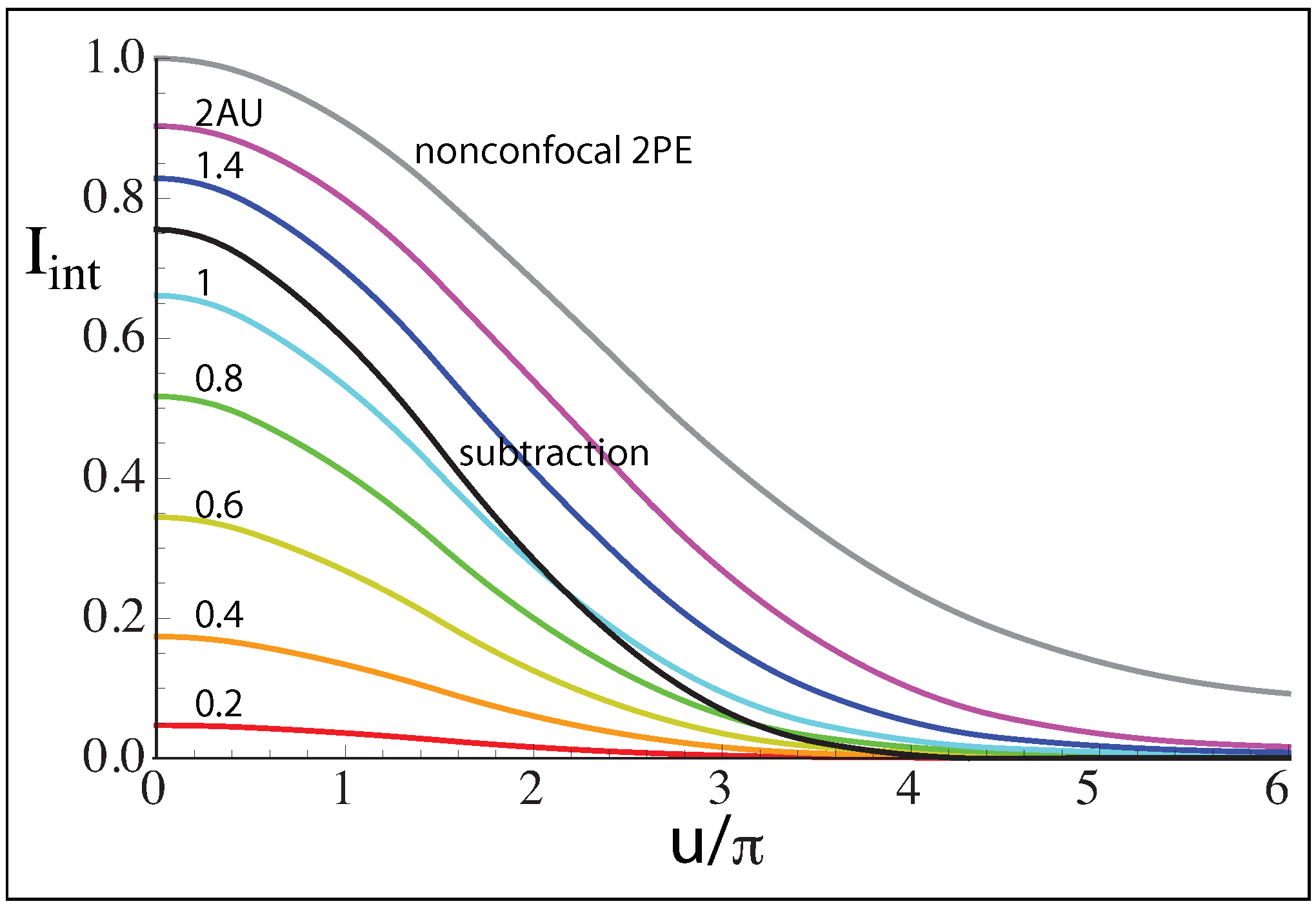
2. Integrated Intensity, Optical Sectioning and Background

In a recent paper, we discussed the properties of integrated intensity, optical sectioning and background in confocal microscopy and ISM [5]. For ISM, I int is equal to that in a confocal microscope, in which the pinhole size is equal to that of the detector array, and it is also independent of any pixel reassignment. The variation in I int with defocus determines the strength of optical sectioning. Conventionally, this is specified by the FWHM 2 u 1 / 2 [2], where the normalized axial distance (in axial optical coordinates) for I int to fall to one half its in-focus value is u 1 / 2 with u = 8 π n z sin 2 α / 2 / λ , where n sin α is the numerical aperture (with α as the angle of convergence of the objective lens and n as the refractive index of the immersion medium) and z is the true axial distance [27]. The variation in integrated intensity with the position, x , in the detector plane and with defocus, u, is what we call the axial fingerprint, F axial ( x , u ) . The background B vol is the signal recorded for a uniform fluorescent volume object and is equal to the axial integral over the axial fingerprint. It is also equal to the integral over the intensity in the detector plane for a fluorescent volume object. Again, it is independent of pixel reassignment. The peak intensity I peak of the image of a fluorescent point object does, however, differ for confocal microscopy and ISM, and it also depends on the PRF. In fact, it can be greater than the peak in a conventional image of a point object as the collected energy is squeezed into a smaller PSF (a property called superconcentration or superbrightness) [22,28]. In addition, in a recent paper, we showed that the outer regions of the detector array tend to detect signals from defocused regions of the sample [5]. This must obviously be the case, as the axial resolution in confocal microscopy is worse for larger pinhole sizes. By processing the signals from different regions of the detector array, optical sectioning can thus be improved [4]. In a previous paper [24], we showed that I peak for a detector point with a large offset can be increased by reassignment to the peak of the PSF rather than to the point midway between the illumination and detection points. While this is valid for a planar object, for a thick object, it is better to treat this measurement as emanating from a defocused object region.
Several papers have discussed the imaging properties of 2PE microscopy in the scalar, paraxial approximation [29,30,31,32,33,34]. We continue to use the scalar, paraxial approximation in this paper for simplicity and in order to make the fundamental behavior more clear. The PSF for a high-numerical aperture polarization theory of confocal 2PE microscopy has also been published [35,36].
An offset point detector gives a true confocal image with a PSF given by the product of the excitation and detection PSFs H 1 H 2 , where they are shifted transversely relative to one another. The intensity PSF for an aberration-free lens with a circular pupil in the scalar, paraxial approximation normalized to unity at the focus is rotationally symmetric and is given by
H ( v ) = 2 0 1 J 0 ( v ρ ) exp 1 2 i u ρ 2 ρ d ρ 2 ,
where J ν is a Bessel function of the first type of order ν and the normalized optical coordinate v = ( 2 π n r sin α ) / λ , where r is the cylindrical radius. The value v = j 11 3.83 , the first zero of J 1 , corresponds to 1 Airy unit (AU). A number of AUs is therefore a dimensionless, normalized radius. The results presented are plotted against u and v or AU. If we know n, α and λ , then they can be converted to true distances z and r.
We assume that the illumination wavelength is twice the 2PE fluorescence wavelength (i.e., we neglect a Stokes shift). By integrating in 2D over the PSF, we can calculate the integrated intensity I int . Figure 1 shows, on a log-log plot, the resulting variation in I int for 2PE with defocus for different offsets, which we call the axial fingerprint. In all cases, the curves are symmetrical about the in-focus plane, where u = 0 . For no offset, the intensity reduces monotonically with defocus, but for offsets larger than about 1.3 AU, the maximum intensity occurs away from the focal plane. For u values larger than about 4 π , I int decays as the fourth power of defocus, an indication of strong optical sectioning, and is approximately independent of the offset. These same data can be displayed in a different format by plotting against the offset with u as a parameter, as shown in Figure 2. It can be seen that for the defocused cases, for larger offsets, the intensity is greater than for the in-focus case such that the signal mainly comes from the defocused regions of the object. Again, it can be seen that the intensity for u = 4 π is almost independent of the offset. Figure 2 can also be interpreted as the variation in intensity in the detector plane for a uniform fluorescent sheet. These two plots are for a single offset point detector, but when we integrate over a ring of point detectors, we must multiply it by the circumference of the ring such that the strength of the total signal for the outer regions of the detector is increased, as shown in Figure 3. Now, even for the in-focus case where u = 0 , the peak occurs at a radius of about 0.6 AU, and thus radii less than this also correspond to the in-focus regions. For a radius of 1.2 AU, the measured signal predominantly comes from regions defocused by u = π or more, and the effective defocus distance increases as the ring radius increases.
Through integration over the rings, the total signal I int for a disk-shaped detector can be determined, as shown in Figure 4. For the single-photon fluorescence, we found that an alternative calculation method using the product of the defocused OTFs of the excitation and detection lenses was more accurate, but the defocused PSFs were difficult to calculate for the 2PE case, and the PSFs decayed more quickly for the 2PE case. Thus, integration over the rings is sufficiently accurate [5,30]. The intensities have been normalized so that for an infinitely large detector corresponding to conventional, non-confocal, 2PE microscopy, I int = 1 . This is different from our previous published treatment [34]. I int decreases smoothly with defocus. The curve for u = 0 has been reported previously [30]. In Figure 4, we also show the behavior of the background from a uniform volume object B vol , which is computed by integration over defocus and again normalized to unity for an infinite pinhole. This curve agrees well with the previously reported results [30]. Even for an infinite detector radius, the integrated intensity decreases with defocus, as there is still an optical sectioning effect from 2PE. Interestingly, the shape of the curve for B vol is very similar to that for I int for u = 5 π / 3 5.24 . This behavior is different from the case of 1PE, where the background from a volume object diverges for an infinite pinhole as there is no optical sectioning [5].
We can calculate the ratios I int / B vol , representing the in-focus signal-to-background ratio ( ( S / B ) axial ), and I int / B vol 1 / 2 , representing the in-focus signal-to-noise ratio ( S / N ) axial (also called the axial detectability D axial ) [34,37]. ( S / B ) axial decays monotonically with an increasing detector size, but ( S / N ) axial is optimized for a detector size of 1.41 AU [34]. The value of ( S / B ) axial is then about 70% greater while ( S / N ) axial is 17% greater than for non-confocal 2PE. Note that these figures are for the axial noise performance compared with the corresponding ( S / B ) 3 D and ( S / N ) 3 D with S = I peak , where the results are very different for confocal microscopy and ISM [34]. Here, ( S / N ) 3 D is called the 3D detectability, also written as D 3 D [37].
The data for I int in Figure 4 can also be replotted against defocus with the detector radius as parameter, as shown in Figure 5. The curves are normalized to unity for an in-focus, non-confocal two-photon microscope. I int decays as 1 / z 4 , compared with 1 / z 2 for non-confocal 2PE microscopy. We can see that for a detector size smaller than 1.4 AU, the signals from defocused regions greater than u = 6 π were very small.

3. Improving Optical Sectioning

As we recognize that the outer regions of the detector measure signals from defocused regions of the object, they can be used to improve further the optical sectioning behavior [4,5]. We see from Figure 2 that the background from regions for u 4 π is spread uniformly over the detector area [38]. The simplest approach is to limit the size of the central area to, for example, 1.4 AU and to subtract a proportion of the signal from an annular region from 1.4 to 2 AU. As these two signal both decay as 1 / z 4 for large z values, we can ensure that these decays cancel, leaving a result that decays approximately as 1 / z 6 while also ensuring that I int does not take negative values and avoiding a major problem of subtractive microscopy. The central disk is also not subtracted, as is the case when two sizes of pinholes are subtracted, and thus the noise performance is improved [39]. We have taken the subtractive factor to be 0.98, with the variation in I int with defocus being shown in Figure 5. Then, B vol = 0.38 so that ( S / B ) axial is improved to 2.0 times and ( S / N ) axial to 1.23 times, the values for nonconfocal 2PE. Here, we have taken into account that subtraction decreases the signal but increases the noise.
I int and B vol are both the same for confocal microscopy and ISM. Furthermore, for ISM, they are independent of the PRF. In ISM, there are various possible strategies for applying the subtractive approach. In Figure 6, we show cross-sections (in the plane containing the direction of offset (x) and the optical axis) through the 3D PSF for 2PE with an offset point detector, given by the product of the excitation and detection PSFs, for different detector offsets. The variation in intensity is symmetrical about the in-focus plane where u = 0 . The coordinate v now represents a normalized x distance and can therefore be negative. No pixel reassignment is assumed. The PSF is less structured than in single-photon fluorescence because the excitation PSF exhibits weak sidelobes [5]. For offsets up to about 0.8 AU, the PSF consists of a single lobe. By 1 AU, two defocused peaks appear. Unlike the single-photon case, these occur only on one side of the main lobe as a result of the two differing excitation and detection PSFs. By 1.5 AU, the two defocused peaks, which occur at u ± 6 , are almost as high as the main lobe. At 2 AU, two pairs of defocused peaks are evident.
These plots are for single-point detectors. Upon integration over a ring of point detectors, the resulting PSF becomes rotationally symmetric and depends strongly on pixel reassignment. Any PRF is a valid reconstruction, with P R F = 0 (no reassignment) corresponding to a confocal system with a finite detector after integration and P R F = 1 corresponding to full-field 2PE [33]. For no pixel reassignment, we rotate the 3D PSF about the axis v = 0 and integrate it. For small offsets, the optimum PRF is 2/3 of the offset [33,34]. In our previous paper, we proposed reassigning the maximum in-focus peak of the PSF to the center of rotation. This maximizes the signal for a planar object but degrades the axial resolution [34]. It is important to appreciate that rotation and integration enhances the region of the PSF near the axis of rotation. Thus, for 1.5 AU, although the main lobe has a height about twice as high as the saddle between the two defocused peaks, after reassignment and integration, it is more than 10 times as high. If, on the other hand, we perform reassignment to bring the defocused peaks to the axis of rotation, corresponding to a PRF of 0.0944, the saddle is twice as high as what was the main peak. The two defocused peaks are now each 1.4 times as high as the in-focus peak. Therefore, integration over a ring of detector elements can image at different depths using the same image data from a single in-focus scan, according to the value of the PRF. This is possible because of the redundancy of image data in ISM. The defocused image is not very good for a 1.5 AU offset but becomes better as the offset increases. However, in the present example, the PSF is symmetrical in the axial direction. Thus, it is not possible to distinguish between positive and negative defocus, and we use the defocus information just to improve optical sectioning. Other works have used a PSF which is not symmetrical in the axial direction in the 1PE case to determine the defocus distances [40].
We use the subtraction described earlier, where the signal from the 1.4 AU disk array is reassigned with a PRF of 2/3, and a factor 0.98 times that from the annulus is subtracted. The annulus, with inner and outer radii of 1.4 and 2 AU, respectively, can be reassigned with various PRFs. After subtraction, the following four strategies (A–D) all give a PSF that is compact and altered only minimally:
A.
If the pixels are reassigned to bring the defocused peaks to the center, then the FWHM of the axial cross-section through the 3D PSF is improved by 6.2% ( I peak = 2.56 ) compared with unity for nonconfocal 2PE, and its smallest negative value is < 2 % .
B.
If, on the other hand, the annulus is reassigned with a PRF of 2/3, the improvement in axial FWHM is < 0.5% ( I peak = 2.48 ) but the negative excursion is only 0.04% .
C.
For P R F = 0 , the improvement in axial FWHM is 2.6% ( I peak = 2.63 ), and the negative excursion is 1.8% .
D.
For P R F = 1 , corresponding to full-field 2PE, the improvement in axial FWHM is 0.2% ( I peak = 2.64 ), and the negative excursion is 0.04% .
All of these approaches give the great improvement in optical sectioning and background suppression described earlier. The performance is summarized in Table 2. It seems that the choice of the PRF for the annulus is not all that important. Reassigning to the defocused peak (A) was difficult to achieve experimentally and had the greatest negative excursion, and P R F = 0 (C) also had a similar negative excursion. Thus, we rejected these two options. The other two options had very small negative excursions. Reassigning to the in-focus peak (B) could be achieved with our existing adaptive pixel reassignment (APR) algorithm [21], and P R F = 1 (D) is simple to perform. Thus, either of these options are attractive, with D being marginally preferable.

4. Discussion

The variation for two-photon excitation in integrated intensity with defocus and an offset detector pixel was plotted. We call this the axial fingerprint F axial . It was shown that the signal from pixels further from the optical axis tended to come from defocused object regions. The variation with defocus in the integrated intensity and volume background B vol for a disk-shaped detector was also shown. It was found that the volume background effectively came from a normalized defocus distance of u = 5.24 . Optical sectioning in a two-photon microscope with a limited detector size is stronger than in either a conventional two-photon microscope or a scanning (1PE) microscope with a limited detector size.
Theer and Denk showed that the imaging depth in non-confocal 2PE is ultimately limited by the near-surface fluorescence [11]. This is exacerbated by the fact that the near-surface fluorescence is collected much more efficiently [10]. Confocal 2PE and 2PE ISM both improve optical sectioning, thus reducing the near-surface fluorescence, but require that ballistic fluorescent photons be detected. Some papers have experimentally demonstrated the improved imaging performance of confocal 2PE microscopy [8,9,10] and ISM [12,13,14,15]. Song et al. in particular claimed an improvement in 2PE imaging depth using a comparatively large confocal pinhole [10].
In the present paper, we have shown that the optimum detector size for axial S/N is much larger than that for 3D S/N (1.41 AU compared with 0.63 AU, respectively) [32]. An improvement in imaging depth in 2PE through background rejection using subtraction of defocused information has been demonstrated both theoretically and experimentally [41,42,43]. Although background rejection is improved dramatically by a combination of ISM and defocus subtraction, an improvement in imaging depth may only result under specific conditions. Nevertheless, within the imaged range of depths, resolution and noise performance should be further improved over ISM alone. Further, more advanced digital processing of the defocused signal, such as focus-ISM [4], should perform better than the simple subtraction method explored here.

Author Contributions

Conceptualization, C.J.R.S., M.C., G.T., A.Z., E.S., P.B., G.V. and A.D.; methodology, C.J.R.S., G.T., A.Z. and G.V.; software, C.J.R.S.; validation, C.J.R.S., A.Z. and G.V.; formal analysis, C.J.R.S.; investigation, C.J.R.S.; resources, C.J.R.S.; data curation, C.J.R.S.; writing—original draft preparation, C.J.R.S.; writing—review and editing, A.Z. and G.V.; supervision, G.V. and A.D.; project administration, G.V. and A.D.; funding acquisition, G.V. and A.D. All authors have read and agreed to the published version of the manuscript.

Funding

This research received no external funding.

Conflicts of Interest

M.C., P.B., A.D. and G.V. have a personal financial interest (co-founders) in Genoa Instruments, Italy.

References

  1. Sheppard, C.J.R.; Choudhury, A. Image formation in the scanning microscope. Opt. Acta 1977, 24, 1051–1073. [Google Scholar] [CrossRef]
  2. Sheppard, C.J.R.; Wilson, T. Depth of field in the scanning microscope. Opt. Lett. 1978, 3, 115–117. [Google Scholar] [CrossRef]
  3. Gu, M.; Sheppard, C.J.R. Effects of finite-sized detector on the OTF of confocal fluorescent microscopy. Optik 1991, 89, 65–69. [Google Scholar]
  4. Tortarolo, G.; Zunino, A.; Fersini, F.; Castello, M.; Piazza, S.; Sheppard, C.J.R.; Bianchini, P.; Diaspro, A.; Koho, S.V.; Vicidomini, G. Focus-ISM for sharp and gentle super-resolved microscopy. Nat. Commun. 2022, 13, 7723. [Google Scholar] [CrossRef]
  5. Sheppard, C.J.R.; Castello, M.; Tortarolo, G.; Zunino, A.; Slenders, E.; Bianchini, P.; Vicidomini, G.; Diaspro, A. Signal strength and integrated intensity in confocal and image scanning microscopy. J. Opt. Soc. Am. A 2023, 40, 138–148. [Google Scholar] [CrossRef]
  6. Sheppard, C.J.R.; Kompfner, R. Resonant scanning optical microscope. Appl. Opt. 1978, 17, 2879–2882. [Google Scholar] [CrossRef]
  7. Denk, W.; Strickler, J.H.; Webb, W.W. Two-photon laser scanning flourescence microscopy. Science 1990, 248, 73–76. [Google Scholar] [CrossRef] [Green Version]
  8. Wang, C.-M.; Fraser, S.E. The resolution improvement in two-photon laser scanning microscopy. In OSA Annual Meeting; Optical Society of America: Washington, DC, USA, 1997; p. 154. [Google Scholar]
  9. Gauderon, R.; Lukins, P.B.; Sheppard, C.J.R. Effect of a confocal pinhole in two-photon microscopy. Microsc. Res. Tech. 1999, 47, 210–214. [Google Scholar] [CrossRef]
  10. Song, W.; Lee, J.; Kwon, H.-K. Enhancement of imaging depth of two-photon microscopy using pinholes: Analytical simulation and experiments. J. Opt. Soc. Am. A 2012, 20, 20605–20622. [Google Scholar] [CrossRef]
  11. Theer, P.; Denk, W. On the fundamental imaging-depth limit in two-photon microscopy. J. Opt. Soc. Am. A 2006, 23, 3139–3149. [Google Scholar] [CrossRef]
  12. Ingaramo, M.; York, A.G.; Wawrzusin, P.; Milberg, O.; Hong, A.; Weigert, R.; Shroff, H.; Patterson, G.H. Two-photon excitation improves multifocal structured illumination microscopy in thick scattering tissue. Proc. Natl. Acad. Sci. USA 2014, 111, 5254–5259. [Google Scholar] [CrossRef] [PubMed] [Green Version]
  13. Gregor, I.; Spieker, M.; Petrovsky, R.; Grosshans, J.; Ros, R.; Enderlein, J. Rapid nonlinear image scanning microscopy. Nat. Methods 2017, 14, 1087–1089. [Google Scholar] [CrossRef] [PubMed]
  14. Sun, S.; Liu, S.; Wang, W.; Zhang, Z.; Kuang, C.F.; Liu, X. Improving the resolution of two-photon microscopy using pixel reassignment. Appl. Opt. 2018, 57, 6181–6187. [Google Scholar] [CrossRef]
  15. Koho, S.V.; Slenders, E.; Tortarolo, G.; Castello, M.; Buttafava, M.; Villa, F.; Tcarenkova, E.; Ameloot, M.; Bianchini, P.; Sheppard, C.J.R.; et al. Two-photon image scanning microscopy with SPAD array and blind image reconstruction. Biomed. Opt. Express 2020, 11, 2905–2924. [Google Scholar] [CrossRef] [PubMed]
  16. Tzang, O.; Feldkhun, D.; Agrawal, A.; Jesacher, A.; Piestun, R. Two-photon PSF-engineered image scanning microscopy. Opt. Lett. 2014, 44, 895–898. [Google Scholar] [CrossRef]
  17. Sheppard, C.J.R. Super-resolution in confocal imaging. Optik 1988, 80, 53–54. [Google Scholar]
  18. Müller, C.B.; Enderlein, J. Image scanning microscopy. Phys. Rev. Lett. 2010, 104, 198101. [Google Scholar] [CrossRef]
  19. Schulz, O.; Pieper, C.; Clever, M.; Pfaff, J.; Ruhlandt, A.; Kehlenbach, R.H.; Wouters, F.; Grosshans, J.; Bunt, G.; Enderlein, J. Resolution doubling in fuorescence microscopy with confocal spinning-disk image scanning microscope. Proc. Natl. Acad. Sci. USA 2013, 33, 21000–21005. [Google Scholar] [CrossRef] [Green Version]
  20. Huff, J. The Airyscan detector from ZEISS: Confocal imaging with improved signal-to-noise ratio and super-resolution. Nat. Methods 2015, 12, i–ii. [Google Scholar] [CrossRef]
  21. Castello, M.; Tortarolo, G.; Buttafava, M.; Deguchi, T.; Villa, F.; Koho, S.; Pesce, L.; Oneto, M.; Pelicci, S.; Lanzano, L.; et al. A robust and versatile platform for image scanning microscopy enabling super-resolution FLIM. Nat. Methods 2019, 16, 175–178. [Google Scholar] [CrossRef]
  22. Sheppard, C.J.R.; Mehta, S.B.; Heintzmann, R. Superresolution by image scanning microscopy using pixel reassignment. Opt. Lett. 2013, 38, 2889–2892. [Google Scholar] [CrossRef] [PubMed]
  23. Sheppard, C.J.R. The development of microscopy for super-resolution: Confocal microscopy, and image scanning microscopy. Appl. Sci. 2021, 11, 8981. [Google Scholar] [CrossRef]
  24. Sheppard, C.J.R.; Castello, M.; Tortarolo, G.; Deguchi, T.; Koho, S.V.; Vicidomini, G.; Diaspro, A. Pixel reassignment in image scanning microscopy: A re-evaluation. J. Opt. Soc. Am. A 2020, 35, 154–162. [Google Scholar] [CrossRef]
  25. Sheppard, C.J.R. Pixel reassignment in image scanning microscopy with a doughnut beam: Example of maximum likelihood restoration. J. Opt. Soc. Am. A 2021, 38, 1075–1084. [Google Scholar] [CrossRef]
  26. Sheppard, C.J.R. Structured illumination microscopy (SIM) and image scanning microscopy (ISM): A review and comparison of imaging properties. Phil. Trans. Royal Soc. A 2022, 76, 379. [Google Scholar]
  27. Sheppard, C.J.R.; Matthews, H. Imaging in high aperture optical systems. J. Opt. Soc. Am. A 1987, 4, 1354–1360. [Google Scholar] [CrossRef]
  28. Roth, S.; Sheppard, C.J.R.; Heintzmann, R. Superconcentration of light—Circumventing the classical limit to achievable irradiance. Opt. Lett. 2016, 41, 2109–2112. [Google Scholar] [CrossRef]
  29. Sheppard, C.J.R.; Gu, M. Image formation in two-photon fluorescence microscopy. Optik 1990, 86, 104–106. [Google Scholar]
  30. Gu, M.; Sheppard, C.J.R. Effects of a finite-sized pinhole on 3-D image formation in confocal two-photon fluorescence microscopy. J. Mod. Opt. 1993, 40, 2009–2024. [Google Scholar] [CrossRef]
  31. Gu, M.; Sheppard, C.J.R. Comparison of three-dimensional imaging properties between two-photon and single-photon fluorescence microscopy. J. Microsc. 1995, 177, 128–137. [Google Scholar] [CrossRef]
  32. Gauderon, R.; Sheppard, C.J.R. Effect of a finite-size pinhole on noise performance in single-, two-, and three-photon confocal fluorescence microscopy. Appl. Opt. 1999, 38, 3562–3565. [Google Scholar] [CrossRef] [PubMed]
  33. Sheppard, C.J.R.; Castello, M.; Tortarolo, G.; Vicidomini, G.; Diaspro, A. Image formation in image scanning microscopy, including the case of two-photon excitation. J. Opt. Soc. Am. A 2017, 34, 1339–1350. [Google Scholar] [CrossRef] [PubMed]
  34. Sheppard, C.J.R.; Castello, M.; Tortarolo, G.; Deguchi, T.; Koho, S.V.; Vicidomini, G.; Diaspro, A. Image scanning microscopy with multiphoton excitation or Bessel beam illumination. J. Opt. Soc. Am. A 2020, 37, 1639–1649. [Google Scholar] [CrossRef]
  35. Higdon, P.D.; Torok, P.; Wilson, T. Imaging properties of high aperture multiphoton fluorescence scanning optical microscopes. J. Microsc. 1999, 193, 127–1411. [Google Scholar] [CrossRef]
  36. Sheppard, C.J.R.; Török, P. The role of pinhole size in high-aperture two- and three-photon microscopy. In Confocal and Two-Photon Microscopy: Foundations, Applications, and Advances; Diaspro, A., Ed.; Wiley Liss: New York, NY, USA, 2002; pp. 127–152. [Google Scholar]
  37. Gan, X.; Sheppard, C.J.R. Detectability: A new criterion for evaluation of the confocal microscopes. Scanning 1993, 15, 187–192. [Google Scholar] [CrossRef]
  38. Sheppard, C.J.R.; Cogswell, C.J.; Gu, M. Signal strength and noise in confocal microscopy: Factors influencing selection of an optimum detector aperture. Scanning 1991, 13, 233–240. [Google Scholar] [CrossRef]
  39. Sheppard, C.J.R.; Cogswell, C.J. Confocal microscopy with detector arrays. J. Mod. Opt. 1990, 37, 267–279. [Google Scholar] [CrossRef]
  40. Roider, C.; Piestun, R.; Jesacher, A. 3D image scanning microscopy with engineered excitation and detection. Optica 2017, 4, 1373–1381. [Google Scholar] [CrossRef]
  41. Leray, A.; Mertz, J. Rejection of two-photon fluorescence background in thick tissue by differential aberration imaging. Opt. Express 2006, 14, 10565–10573. [Google Scholar] [CrossRef] [Green Version]
  42. Si, K.; Gong, W.; Chen, N.G.; Sheppard, C.J.R. Two-photon focal modulation microscopy in turbid media. Opt. Lett. 2011, 99, 233702. [Google Scholar] [CrossRef]
  43. Zheng, Y.; Chen, J.; Shi, X.; Zhu, X.; Wang, J.; Huang, L.; Si, K.; Sheppard, C.J.R.; Gong, W. Two-photon focal modulation microscopy for high-resolution imaging in deep tissue. J. Opt. Soc. Am. A 2019, 12, e201800247. [Google Scholar] [CrossRef] [PubMed] [Green Version]
Figure 1. A log-log plot of the variation in integrated intensity with defocus for different point detector offsets. We call this the axial fingerprint. The integrated intensity is equivalent to the intensity from a fluorescent sheet object. For a large offset, the integrated intensity decays as the fourth power of defocus, an indication of strong optical sectioning. For offsets larger than about 1.3 AU, the maximum intensity occurs away from the focal plane.
Photonics 10 00601 g001
Figure 2. The variation in intensity in the detector plane for a fluorescent sheet object with different defocus values. This is equal to the integrated intensity for a point object and an offset point detector. For larger offsets, the intensity is greater for the defocused cases than the in-focus case. For u = 4 π , the intensity is almost independent of the offset.
Photonics 10 00601 g002
Figure 3. The integrated intensity I int for a ring of detectors. For a given ring radius larger than about 1.2 AU, the greatest contribution to I int comes from the defocused regions of the object.
Photonics 10 00601 g003
Figure 4. The variation in integrated intensity for a detector disk, with the radius of the disk for different defocus values. The integrated intensity increases monotonically with the detector disk radius. Even for an infinite detector radius, the integrated intensity decreases with defocus, as there is still an optical sectioning effect from 2PE. The background from a volume object is also shown, being very similar to that for I int for u = 5 π / 3 5.24 .
Photonics 10 00601 g004
Figure 5. The integrated intensities for disk detectors of various sizes, including nonconfocal 2PE, as a function of defocus, normalized to unity for an in-focus, non-confocal two-photon microscope. All the curves decay monotonically with defocus. For nonconfocal 2PE, for large defocus values, the integrated intensity decays as the square of the defocus value. For finite-sized detectors, the integrated intensity decays as the fourth power of defocus. The integrated intensity, after subtracting 0.98 times the signal from an annular detector, outer radius 2 AU and inner radius 1.4 AU, from that from a disk detector radius 1.4 AU, labeled “subtraction”, is also shown.
Photonics 10 00601 g005
Figure 6. Cross-sections through the 3D PSF for two-photon excitation and an offset point detector without pixel reassignment for different detector offsets: (top left) 0.5 AU; (top right) 1 AU; (bottom left) 1.5 AU; and (bottom right) 2 AU. The cross-section is the plane containing the direction of offset and the optical axis, and v represents a normalized x distance.
Photonics 10 00601 g006
Table 1. Nomenclature.
VariableDescription
B vol Background from a uniform volume object.
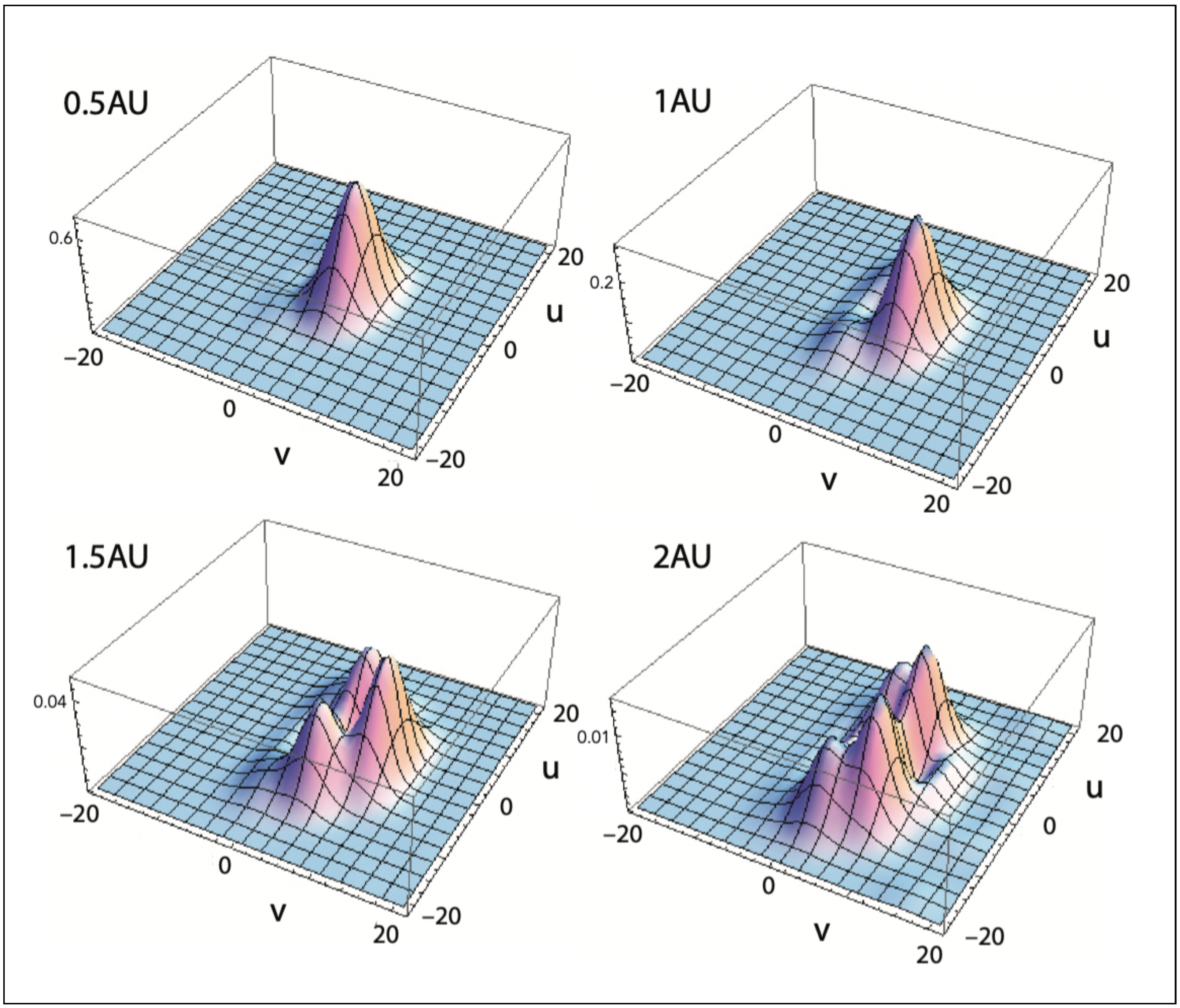
F axial Axial fingerprint: I int variation with defocus for an offset detector point.
I int Integrated intensity: The transverse integral over the PSF.
I peak Peak of the intensity PSF.
HIntensity point spread function (PSF).
uNormalized axial distance (defocus).
u 1 / 2 Value of u for the intensity to drop to 1/2.
vNormalized cylindrical radius r (or normalized distance x).
Table 2. Performance of different reassignment strategies for the annular elements.
StrategyAnnulus PRFImprovement in FWHMI peak Negative Excursion
ADefocused max.6.2%2.56< 2 %
B2/3< 0.5% 2.48 0.04%
C0 2.6% 2.63 1.8%
D1 0.2% 2.64 0.04%
Disclaimer/Publisher’s Note: The statements, opinions and data contained in all publications are solely those of the individual author(s) and contributor(s) and not of MDPI and/or the editor(s). MDPI and/or the editor(s) disclaim responsibility for any injury to people or property resulting from any ideas, methods, instructions or products referred to in the content.

