Study on the Influence of Underwater LED Illumination on Bidirectional Underwater Wireless Optical Communication

Abstract

Underwater wireless optical communication (UWOC) is acknowledged as a useful way to transmit data in the ocean for short-distance applications. Carrying a UWOC device on mobile platforms is quite practical in ocean engineering, which is helpful to exploit its advantages. In application, such a platform needs a camera to observe the surroundings and guide its action. Since the majority of ocean is always dark, active illumination is necessary to imaging. When UWOC works in such an environment, its performance is affected by the illumination light noise. In this paper, we study the influence of underwater LED illumination on bidirectional UWOC with the Monte Carlo method. We simulate forward noise from LED illumination to the opposite receiver in the cooperative terminal, and the backscattering noise on the adjacent receiver in the same terminal. The results show that the forward noise is reduced with the increase of theabsorption coefficient, scattering coefficient, transmitting distance, and separated distance between receiver and the optical axis of LED. However, it becomes greater with the field of view (FOV) of the receiver. The backscattering noise is reduced with the increase of the absorption coefficient and separated distance between receiver and LED. However, it becomes greater with the FOV and scattering coefficient, while it has little relation with transmitting distance. In order to reduce these two kinds of noises, besides inserting an optical filter in the receivers and narrowing their FOV, the optical axis of LED light should keep away from the receivers. The results in this paper are helpful for UWOC application.

1. Introduction

Underwater wireless optical communication (UWOC) is a useful way to transmit data for short distance applications in the ocean, thanks to its high transmission speed [1,2,3]. Recently, many researchers have focused on this topic. They are mainly investigating increasing the communication rate with high-order modulation [4,5,6,7] and high-performance devices [8], or improving the communication distance with a high sensitivity detector [9] and photon counting detection [10,11]. Meanwhile, in the area of ocean engineering, several sea trials have demonstrated its potential application prospects. From 2008 to 2014, Woods Hole Oceanographic Institution (WHOI) demonstrated the value of this technology in deep sea with up to 10M bps speed, more than 100 m distance, and more than 2000 m depth [12,13,14,15,16]. In these trials, UWOC devices were usually carried on mobile platforms, such as human occupied vehicles (HOV), remote operated vehicles (ROV) and autonomous underwater vehicles (AUV). They demonstrate the potential value of using such technology to harvest data from subsea nodes and seafloor observatories by AUV and optical modem [12,13,14], or transmitting data between ROV, HOV, and other underwater platforms [15,16]. Using the same technical scheme, commercial UWOC products have been applied in ocean engineering with up to 10M bps rate. It has been used to stream ocean exploration missions live [17]. Furthermore, in 2017, the Japan Agency for Marine-Earth Science and Technology (JAMSTEC) demonstrated 20M bps speed with 120 m distance in dark clear water. In the system, the UWOC device was carried on an ROV [18].

These sea trials show that carrying the devices on mobile platform is a practical application of UWOC. In this way, UWOC devices can move underwater to establish optical communication links with cooperative targets, which is helpful to exploit its advantages. However, while UWOC devices and such platforms work in the ocean, they usually need a camera to observe the surroundings and guide their action. In this situation, because the majority of ocean is always dark [19], active illumination is necessary for imaging. When UWOC works in such an environment, the illumination light affects its performance, and can even make it unworkable. Therefore, it is necessary to study the influence of light illumination on UWOC. As an underwater light emitting diode (LED) is usually applied to illumination, in this work, we analyze the influence of such light on bidirectional UWOC with the Monte Carlo method.

The organization of this paper is as follows: Section 2 sets up a theoretical model to study light noise with the Monte Carlo method. Section 3 demonstrates the simulation results. Section 4 makes a conclusion.

2. Theoretical Model

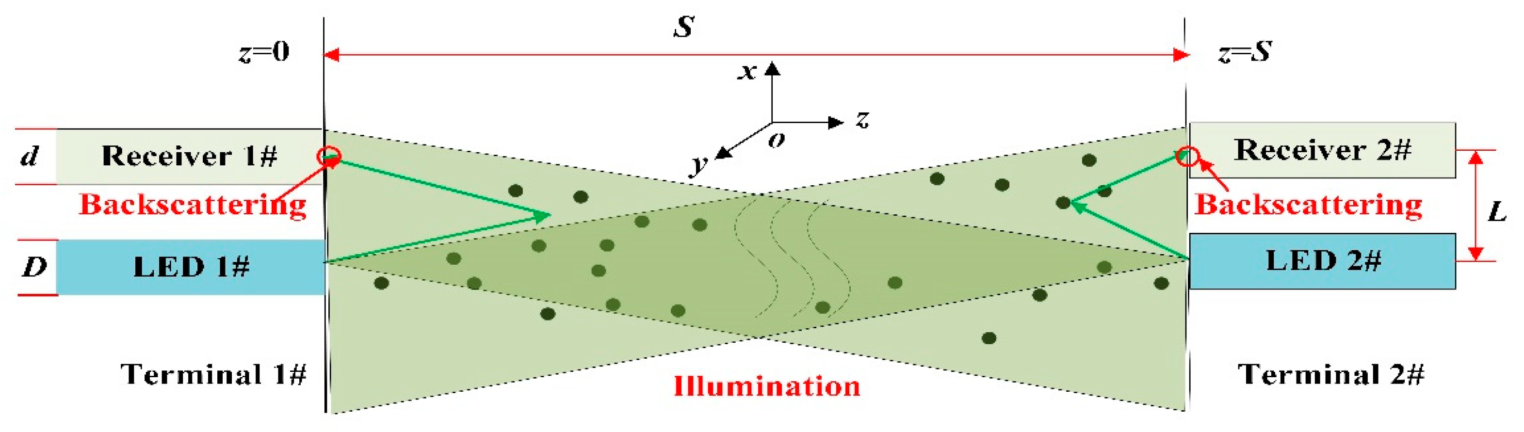
The simulation model is shown in Figure 1. It has two identical terminals, the distance between which is S. In each terminal, there is a UWOC transmitter, a UWOC receiver, and an underwater LED device. In the two terminals, the diameters of the luminous surface for LEDs are both D. The diameters of the UWOC receivers are both d. The separated distances between the UWOC receiver and LED are both L. When the LEDs and UWOC system work simultaneously, the illumination noise would arrive to both the two receivers, because there is scattering in the water. For example, light from “LED 1#” in Figure 1 affects “Receiver 1#” and “Receiver 2#” simultaneously.

We simulated such influence with the Monte Carlo method. This method is quite popular to study underwater optical channels [20]. It is based on the fact that light is made up of many photons. Supposing the process of light propagating underwater is a linear time-invariant system, the transmitting characteristic of every photon follows the same statistical rule. Thus, by tracing the photons’ paths underwater one by one and counting their characteristics, the light feature can be obtained. For example, the time-domain feature of light can be analyzed by counting the photons’ optical path underwater, while the characteristics of the light field can be studied by counting the photons’ positions. In this paper, in order to study the influence of LED illumination noise on UOWC receiver, we count the photons from LED into receivers with different positions. There are three steps.

(1) The process of photons from LED into water is simulated one by one. The coordinates at which that the photons arrived at the plane of the two UWOC receivers are recorded.

(2) The photons whose coordinates are in the receiving surface of UWOC receivers and arriving angle is within the field of view (FOV) of receiver are counted. Then, the number of photons arrived at the receivers is acquired, which includes the opposite receiver in the cooperative terminal and the adjacent receiver in the same terminal.

(3) The numbers of photons arrived at the receivers are divided by the total number we simulated. Then, the relative intensity in the two receivers is obtained. They can be used to evaluate the forward noise from LED illumination to the opposite receiver and backscattering noise to the adjacent receiver, respectively.

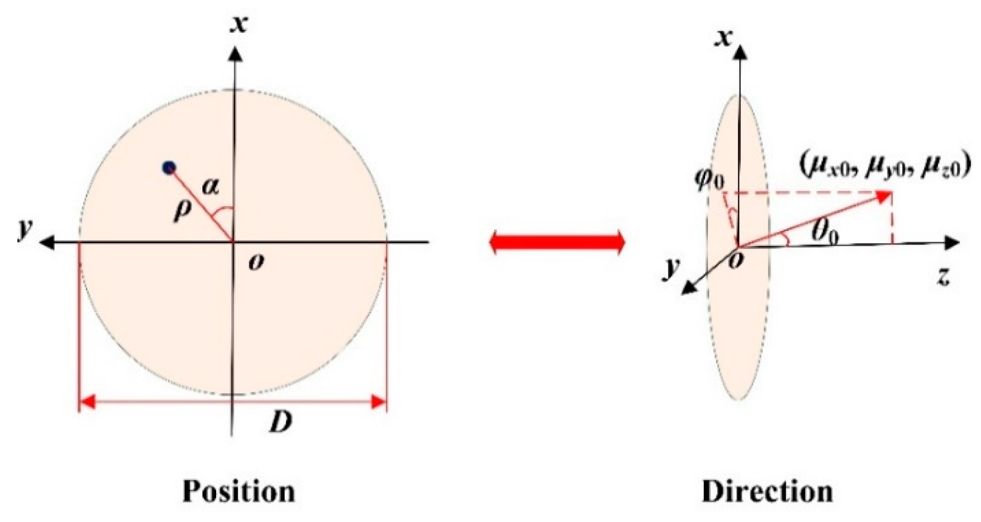
As shown in Figure 1, for simplicity, we study the influence of light from “LED 1#” on “Receiver 1#” and “Receiver 2#”. As shown in Figure 2, this is supposing the luminous surface of “LED 1#” is uniform and round with diameter D. We establish coordinate system with the center of “LED 1#”. Photons’ position and direction cosine are expressed as follows.

$$\left\{\begin{array}{c}{x}_0=\rho \times \cos \alpha =\frac{D}{2}\times \sqrt{ran{d}_r}\times \cos \left({360}^{\circ }\times ran{d}_J\right)\hfill \\ y_0=\rho \times \sin \alpha =\frac{D}{2}\times \sqrt{ran{d}_r}\times \sin \left({360}^{\circ }\times ran{d}_J\right)\hfill \\ z_0=0\hfill \end{array}\right.$$

(1)

$$\left\{\begin{array}{c}{\mu }_{x0}=\sin {\phi }_0\sin {\theta }_0=\sin \left({360}^{\circ }\times ran{d}_{\phi }\right)\times \sin {\theta }_0\hfill \\ {\mu }_{y0}=\cos {\phi }_0\sin {\theta }_0=\cos \left({360}^{\circ }\times ran{d}_{\phi }\right)\times \sin {\theta }_0\hfill \\ {\mu }_{z0}=\cos {\theta }_0\hfill \end{array}\right.$$

(2)

Here, (ρ, α) is the polar coordinate for the photon position in the plane z = 0. θ₀ and φ₀ are theelevation angle and azimuth angle for the starting direction. rand_r, rand_J, and rand_φ are random numbers, which follow uniform distribution in range of 0 and 1. Random numbers are produced by a computer, which will appear in several places below in the model.

The light intensity of LED usually follows Lambert distribution. Its radiation intensity I(θ₀) with an elevation angle θ₀ can be expressed as follows,

$$I({\theta }_0)=I_0\cos {\theta }_0$$

(3)

where I₀ is the intensity at θ₀ = 0. Furthermore, it can be understood that the photon probability density at θ₀ is cos θ₀. Then, a random number rand_θ can be produced with an arbitrary θ₀, as shown in Equation (4).

$${\displaystyle {\int }_0^{{\theta }_0}\cos \xi d}\xi =\sin {\theta }_0=ran{d}_{\theta }$$

(4)

In Equation (4), rand_θ is a random number, which follows uniform distribution in the range of 0 and 1. Therefore, θ₀ can be expressed as follow.

$${\theta }_0=\arcsin \left(ran{d}_{\theta }\right)$$

(5)

Once a photon leaves “LED 1#”, it will transmit straight in water until arriving at the scattering particle. The free path s is

$$s=\frac{-1}{c}\ln \left(ran{d}_s\right)=\frac{-1}{a+b}\ln \left(ran{d}_s\right)$$

(6)

Here a, b, and c are the absorption coefficient, scattering coefficient, and attenuation coefficient of water, respectively. rand_s is a random number. Then, the new position (x, y, z) for photon is

$$\left\{\begin{array}{c}x=x_0+{\mu }_{x0}s\\ y=y_0+{\mu }_{y0}s\\ z=z_0+{\mu }_{z0}s\end{array}\right.$$

(7)

Once z ≤ S and z ≥ 0, the photon will be absorbed or scattered in water, which is determined with the method of “Russian roulette”. That means we firstly should define a threshold W_H as follows:

$$W_{\mathrm{H}}=\frac{b}{c}$$

(8)

Then, we produce a random number rand_W from computer. If rand_W > W_H, the photon is absorbed. We stop the tracing process. Otherwise, it is scattered, the new direction (μ_x, μ_y, μ_z) of which is as follows:

$$\begin{array}{c}\left.\begin{array}{c}{\mu }_x=\frac{\sin \theta }{\sqrt{1-{\mu }_{z0}^2}}\left({\mu }_{x0}{\mu }_{z0}\cos \phi -{\mu }_{y0}\sin \phi \right)+{\mu }_{x0}\cos \theta \\ {\mu }_y=\frac{\sin \theta }{\sqrt{1-{\mu }_{z0}^2}}\left({\mu }_{y0}{\mu }_{z0}\cos \phi +{\mu }_{x0}\sin \phi \right)+{\mu }_{y0}\cos \theta \\ {\mu }_z=-\sin \theta \cos \phi \sqrt{1-{\mu }_{z0}^2}+{\mu }_{z0}\cos \theta \end{array}\right\}\left|{\mu }_{z0}\right|<1\\ \left.\begin{array}{c}{\mu }_x=\sin \theta \cos \phi \\ {\mu }_y=\sin \theta \sin \phi \\ {\mu }_{\mathrm{z}}={\mu }_{z0}\cos \theta \end{array}\right\}\left|{\mu }_{z0}\right|=1\end{array}$$

(9)

φ and θ are the azimuth and scattering angle, respectively. We suppose φ obeys uniform distribution as shown in Equation (10), in which rand_φ1 is a random number.

$$\phi ={360}^{\circ }\times ran{d}_{\phi 1}$$

(10)

θ is determined by the volume scattering function (VSF). There are several models for it, such as the Petzold average particle phase function, Fournier- Forand (FF) function, Henyey–Greenstein (HG) function and its related approximations, etc. Only the HG function can give an analytical expression for scattering angle in a Monte Carlo simulation [20,21]. Although some research indicates that the function value in this model is less than the real water with the scattering angle close to zero or in the backward direction, the simulation error is acceptable in most cases. Hence, we will use the HG function to generate the scattering angle as shown in Equation (11), not only for simplicity, but also because the analytical expression is useful to reduce the computing error in simulation.

$$\cos \theta =\frac{1}{2g}\left[1+g^2-{\left(\frac{1-g^2}{1-g+2g\times ran{d}_{\theta 1}}\right)}^2\right]$$

(11)

g is the asymmetry parameter that depends on the characteristics of medium, which equals to the average cosine of the scattering angle over all scattering directions. In this paper, we set g = 0.924, because it is considered as a good approximation for most practical situations [22]. rand_θ1 is a random number. Then, the process of a photon’s motion in water can be described with Equations (1)–(11).

Once z ≤ 0, we modify the coordinate to the plane z = 0 by Equation (12). We can use these photons to study the backscattering noise from “LED 1#” on “Receiver 1#”. If z ≥ S we modify the coordinate to the plane z = S by Equation (13). We can use these photons to study the noise from “LED 1#” on “Receiver 2#”. Then, illumination from the forward light and backscattering noise on receivers are both acquired.

$$\begin{array}{l}{s}^{\prime }=s\left|\frac{0-z_0}{z-z_0}\right|\\ \left\{\begin{array}{c}{X}_1=x_0+{\mu }_x{s}^{\prime }\\ Y_1=y_0+{\mu }_y{s}^{\prime }\\ Z_1=z_0+{\mu }_z{s}^{\prime }\end{array}\right.\end{array}$$

(12)

$$\begin{array}{l}{s}^{\prime }=s\left|\frac{S-z_0}{z-z_0}\right|\\ \left\{\begin{array}{c}{X}_1=x_0+{\mu }_x{s}^{\prime }\\ Y_1=y_0+{\mu }_y{s}^{\prime }\\ Z_1=z_0+{\mu }_z{s}^{\prime }\end{array}\right.\end{array}$$

(13)

The light distribution from “LED1#” is usually symmetrical to the center. We set the center of “Receiver 1#” and “Receiver 2#” at coordinates (0, L, 0) and (0, L, S) for simplicity. If a photon’s coordinate (X₁, Y₁, Z₁) satisfy Equation (14), and its arriving angle to the receiver is within the field of view (FOV), we record it and stop the tracing.

$${(X_1-0)}^2+{(Y_1-L)}^2\le {\left(\frac{d}{2}\right)}^2$$

(14)

Here, d is the diameter of receiver. We denote the total number of tracing photons as N. If the number of photons arrived at “Receiver 2#” and “Receiver 1#” are N_F and N_B, respectively. The relative intensity η_F and η_B are denoted as Equations (15) and (16), which can be used to evaluate the forward noise from LED illumination to the opposite receiver and backscattering noise to the adjacent receiver.

$${\eta }_{\mathrm{F}}=\frac{N_{\mathrm{F}}}{N}$$

(15)

$${\eta }_{\mathrm{B}}=\frac{N_{\mathrm{B}}}{N}$$

(16)

3. Simulation Result

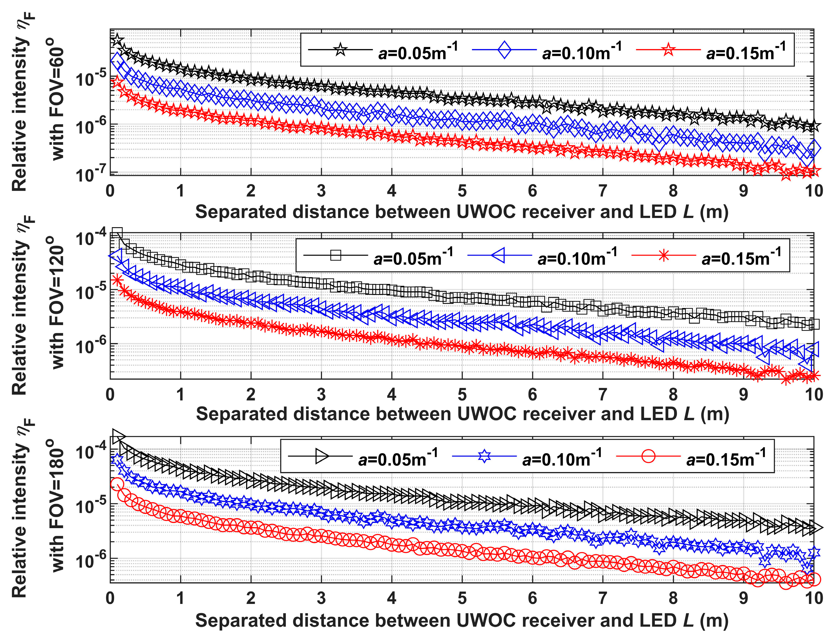
In order to study the influence of illumination noise, we set the diameter of the luminous surface D as 0.1 m for “LED 1#”, the diameter d of “Receiver 1#” and “Receiver 2#” as 0.1 m, and the total number N of tracing photons as 10⁹. Then, we analyze the variation of relative intensity η_B and η_F with the separated distance L from UWOC receiver to the optical axis of LED light, by setting a different absorption coefficient a, scattering coefficient b, transmitting distance S, and FOV of the receiver.

3.1. Analysis of the Influence of Illumination Noise with Different Absorption Coefficient

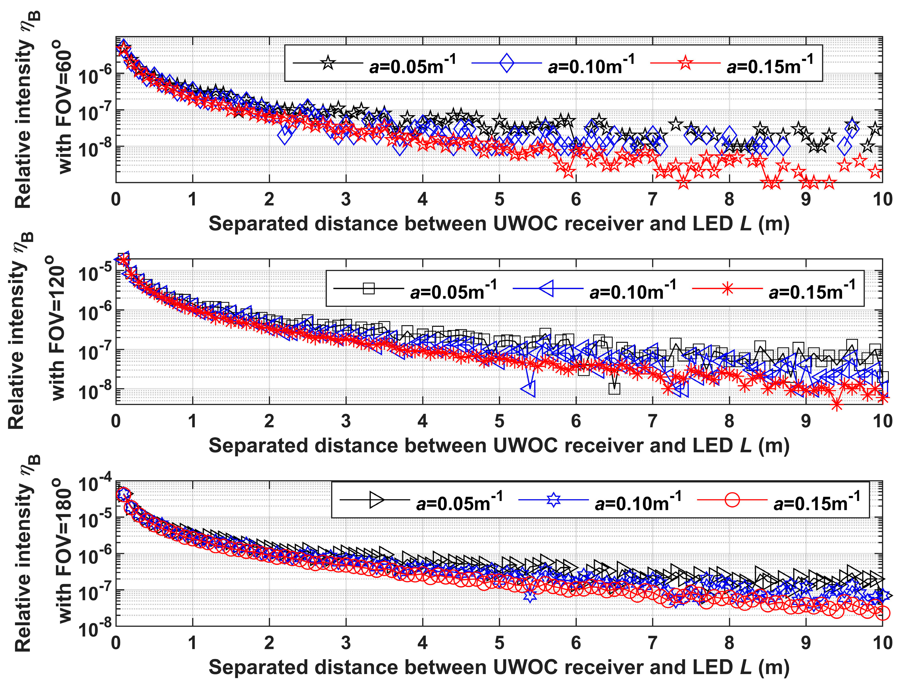
In the real ocean, the absorption coefficient and scattering coefficient (a, b) are different with water [20], which can be close to zero and larger than one. Then, the communication distance S is inconstant. Usually, the UWOC system is suitable for relatively clean water. Therefore, we set b = 0.10 m⁻¹, S = 20 m, while a = 0.05 m⁻¹, 0.10 m⁻¹, and 0.15 m⁻¹, respectively. Then, we count the number of photons arriving at “Receiver 2#” and “Receiver 1#” to calculate the relative intensity η_F and η_B, when FOV is 60°, 120°, and 180°, respectively. The results η_F and η_B vary with L and are shown in Figure 3 and Figure 4, respectively.

In Figure 3 and Figure 4, the general tendency of η_F and η_B versus L is decreasing and the tendency of η_B is more evident. When absorption coefficient a is greater, or the FOV is smaller, the relative intensity η_F and η_B would be smaller. Furthermore, the absorption coefficient has a greater effect on η_F, while the FOV has more influence on η_B.

It needs to be noted here that, in Figure 4, when L is larger or a is smaller, the monotonicity of the curves is not perfect. This is because the number of tracing photons is 10⁹ in the simulation. When L is larger or a is smaller, the number of photons arrived at the receiver is very small. Then, the error is larger. This is caused by the Monte Carlo method itself because it uses a stochastic process to study a physical problem. The accuracy is determined by the sample size. We tried to increase the number of tracing photons to 10¹⁰ to reduce this error. The computing time increased tremendously. The monotonicity of the curves became better, but the error still existed. If the number became larger, the monotonicity would be more perfect, but the error could not be removed thoroughly. As the monotonicity of curves in Figure 4 is modified with the number of tracing photons, the tendency we observe here is credible. This kind of situation would exist in the following simulation.

Therefore, we conclude that the forward noise from LED illumination to the opposite receiver and backscattering noise to the adjacent receiver are both decreasing with the absorption coefficient and the change of forward noise is more evident. Narrowing the receiver’s FOV would reduce such noises. Enlarging the separated distance between receivers and the optical axis of LED would reduce such noises too, while it is more evident to backscattering noise.

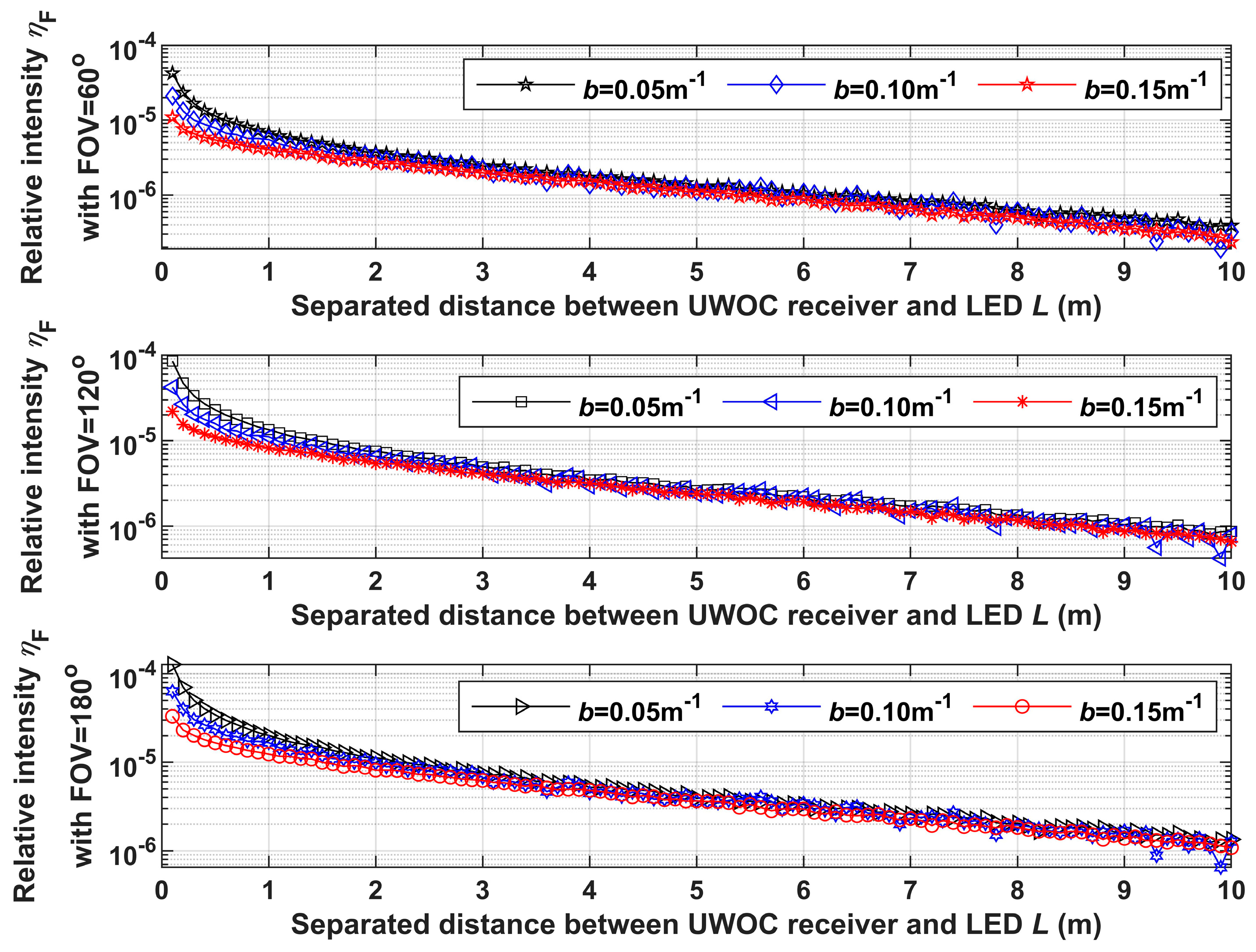
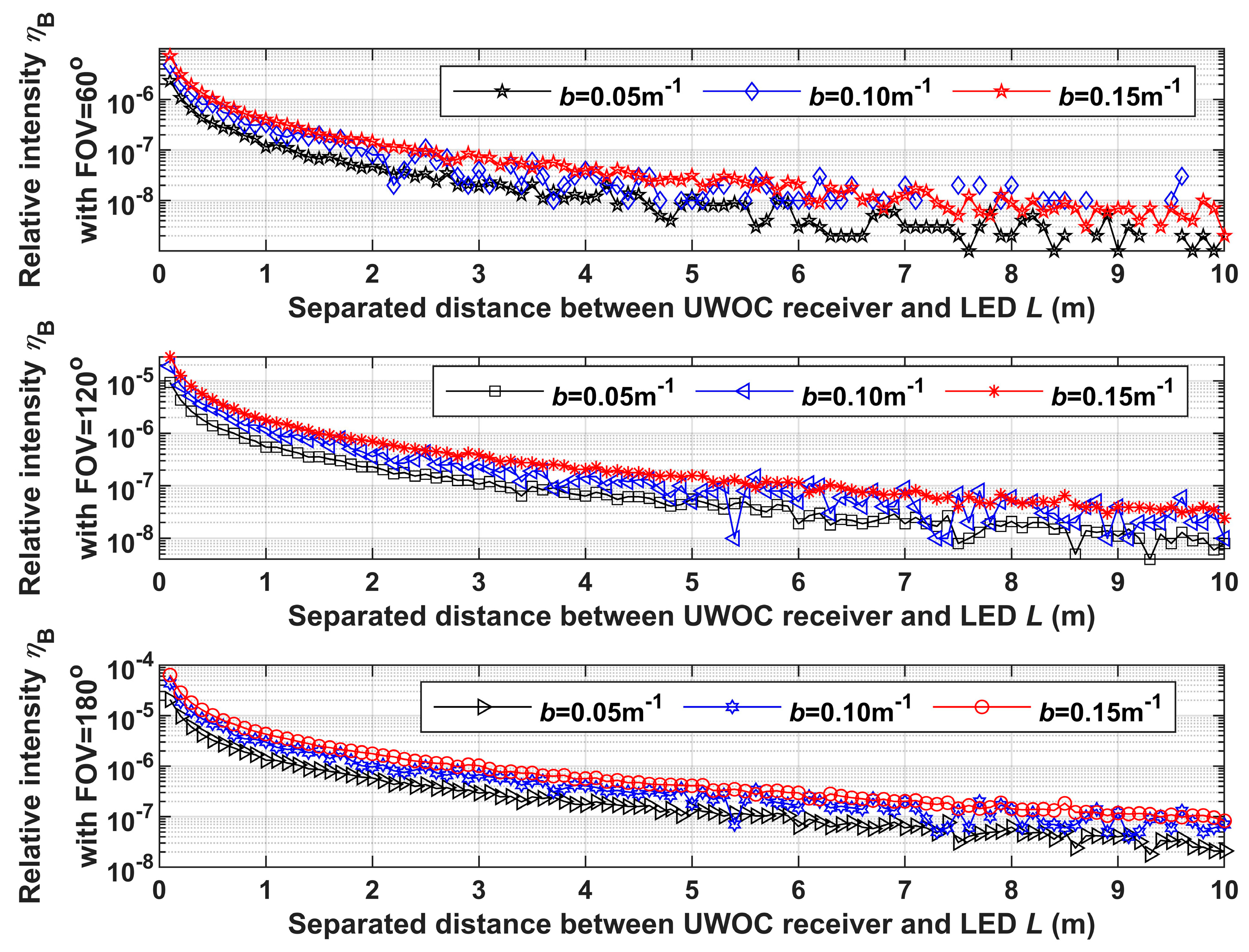
3.2. Analyze the Influence of Illumination Noise with Different Scattering Coefficient

We set a = 0.10 m⁻¹, S = 20 m, while b = 0.05 m⁻¹, 0.10 m⁻¹ and 0.15 m⁻¹, respectively. Then, we count the number of photons arriving at “Receiver 2#” and “Receiver 1#” to calculate the relative intensity η_F and η_B, when the FOV is 60°, 120°, and 180°, respectively. The results η_F and η_B vary with L and are shown in Figure 5 and Figure 6, respectively.

In Figure 5, with the increase of the separated distance L, the relative intensity η_F decreases. When the scattering coefficient b is greater, or the FOV is smaller, the relative intensity η_F is smaller. At a smaller FOV and at larger distances, the relative intensities converge for different scattering coefficients. The difference is quite small. In Figure 6, with the increase of the separated distance L, the relative intensity η_B decreases. Its tendency is more evident than η_F, especially at a smaller FOV and at larger distances. When the scattering coefficient b and the FOV are smaller, the relative intensity η_F is smaller.

Therefore, we conclude that the forward noise from LED illumination to the opposite receiver decreases with the scattering coefficient, while the backscattering noise to the adjacent receiver increases with it. Narrowing the receiver’s FOV would reduce such noises, while the effect is more evident with backscattering noise. Enlarging the separated distance between receivers and the optical axis of LED would reduce such noises too, while it is more evident to backscattering noise.

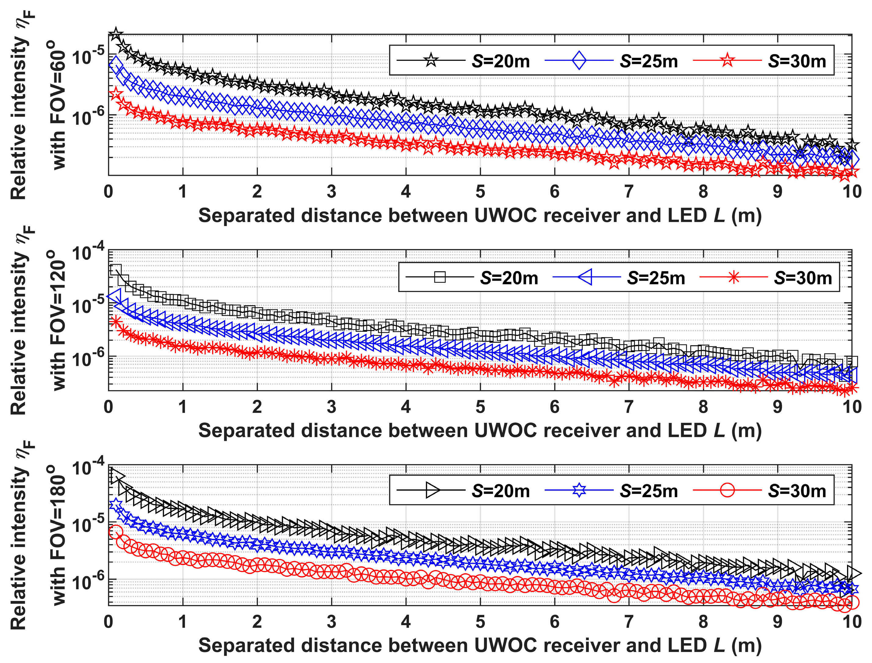
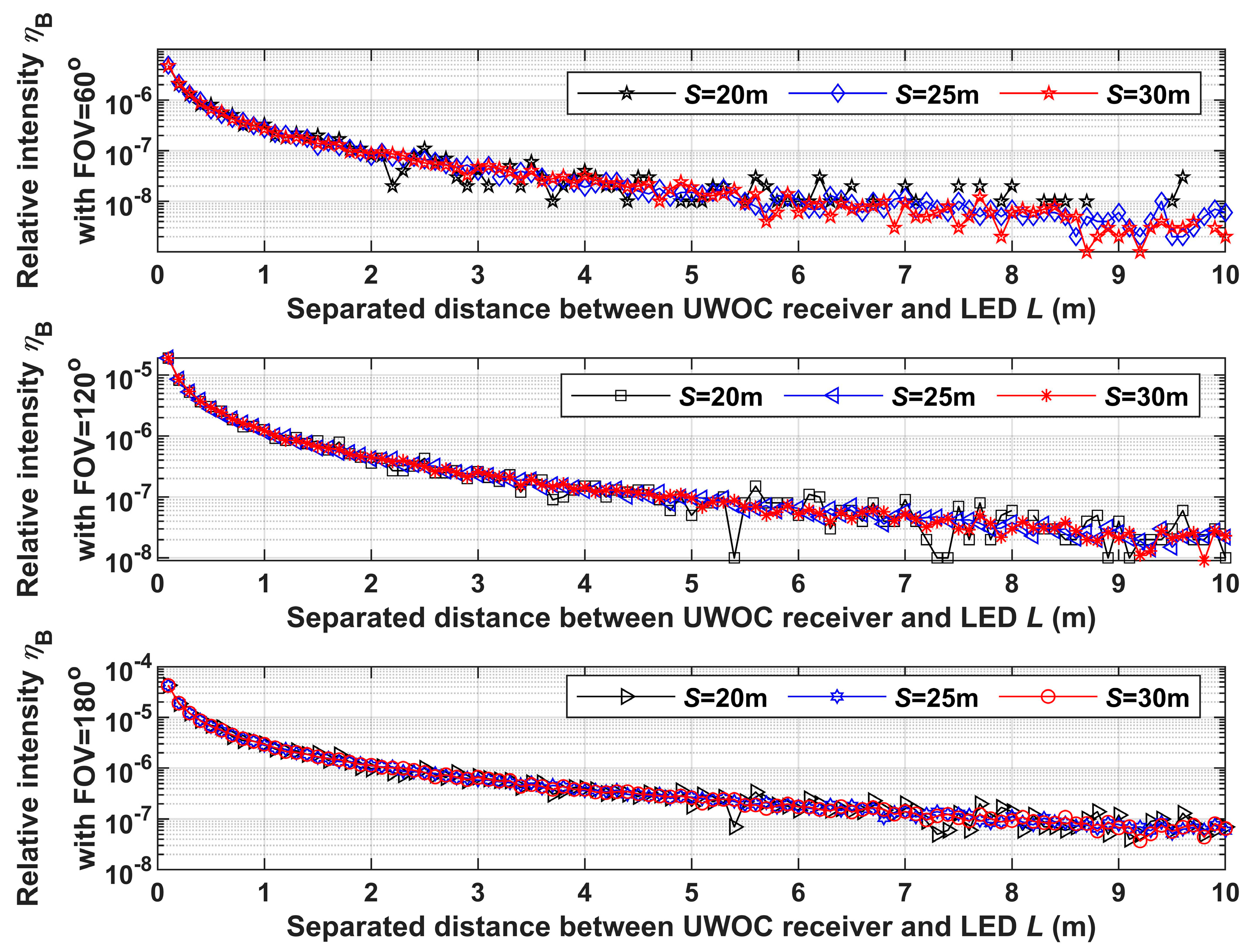
3.3. Analyze the Influence of Illumination Noise with Different Transmitting Distance

We set a = 0.10 m⁻¹, b = 0.10 m⁻¹, and S = 20 m, 25 m, and 30 m, respectively. Then, we count the number of photons arriving at “Receiver 2#” and “Receiver 1#” to calculate the relative intensity η_F and η_B, when FOV is 60°, 120°, and 180°, respectively. The results η_F and η_B vary with L and are shown in Figure 7 and Figure 8 respectively.

In Figure 7, with the increase of separated distance L, the relative intensity η_F decreases. When the transmitting distance S is greater, or the FOV is smaller, the relative intensity η_F is smaller. In Figure 8, with the increase of separated distance L, the relative intensity η_B decreases and its tendency is more evident than η_F. When the FOV is smaller, the relative intensity η_F is smaller too. When the transmitting distance S varies, η_F nearly has no change.

Therefore, we conclude that the forward noise from LED illumination to the opposite receiver decreases with the transmitting distance, while the backscattering noise to the adjacent nearly has no relation with it. Narrowing the receiver’s FOV would reduce such noises, while the effect is more evident with backscattering noise. Enlarging the separated distance between receiver and the optical axis of LED would reduce such noises too, while it is more evident with backscattering noise.

3.4. Discussion

From the results above, it is clear that forward noise from the LED illumination affects the opposite receiver, while the backscattering noise impacts the adjacent receiver in the same terminal. With the increase of separated distance between receiver and the optical axis of LED, both the noises decrease. The tendency is more evident for the backscattering one. With the increase of absorption coefficient, the two noises are decreased, while the change of the forward noise is more evident. With the increase of scattering coefficient, the forward noise to the opposite receiver decreases, while the backscattering noise to the adjacent receiver increases. With the increase of the transmitting distance, the forward noise to the opposite receiver decreases, while the backscattering noise to the adjacent nearly has no change. With the increase of FOV, both the noises increase. What needs illustration is that when we change other simulation parameters, such results still stand.

The simulation results above can be explained theoretically. For the opposite receiver, the forward noise is determined by the loss in the transmitting channel. When increasing the absorption coefficient, scattering coefficient, transmitting distance, and the separated distance between receiver and the center of LED illumination, or narrowing the FOV of receiver, the loss becomes greater. Then, the forward noise is less.

For the adjacent receiver in the same terminal, the backscattering noise is mainly determined by the backscattering light near the receiver. When the absorption coefficient enlarges, the noise light into receiver reduces a little. When the scattering coefficient enlarges, the backscattering becomes more evident and the noise is increased. When the transmitting distance increases, the backscattering has little change. When FOV reduces, or the separated distance between receiver and the center of LED increases, less light comes into the receiver.

Furthermore, from the results above, it is clear that backscattering noise from LED illumination to the adjacent receiver in the same terminal cannot be neglected in application, in particular when there is strong scattering in the water.

In order to reduce such light noise from LED illumination, besides inserting an optical filter in the receivers, the FOV should be smaller and the separated distance between receiver and the center of LED illumination should be longer. These two methods are more useful to the backscattering noise of the adjacent receiver.

4. Conclusions

In this paper, we study the influence of underwater LED illumination on bidirectional UWOC. Firstly, we establish a theoretical model with the Monte Carlo method. Then, we simulate forward noise from the LED illumination to the opposite receiver, and the backscattering noise on the adjacent receiver in the same terminal. The results show that the forward noise is reduced with the absorption coefficient, scattering coefficient, transmitting distance, separated distance between receiver, and the optical axis of LED, but becomes greater with FOV of receiver. The backscattering noise is reduced with absorption coefficient and separated distance between the receiver and LED, but becomes greater with the FOV of receiver and scattering coefficient, while it has little relation with transmitting distance. In order to reduce such these two kinds of noises, besides inserting an optical filter in the receivers, the FOV should be smaller and the separated distance between receiver and the center of LED illumination should be longer, especially for backscattering. The results in this paper are helpful for the application of UWOC. In the future, we will design a UWOC system with LED illumination based on these results.